HAL Id: hal-02545588
https://hal.univ-reunion.fr/hal-02545588
Submitted on 17 Apr 2020
HAL is a multi-disciplinary open access
archive for the deposit and dissemination of
sci-entific research documents, whether they are
pub-lished or not. The documents may come from
teaching and research institutions in France or
abroad, or from public or private research centers.
L’archive ouverte pluridisciplinaire HAL, est
destinée au dépôt et à la diffusion de documents
scientifiques de niveau recherche, publiés ou non,
émanant des établissements d’enseignement et de
recherche français ou étrangers, des laboratoires
publics ou privés.
seismic observations, oceanographic records and offshore
wave models
Elisa Josia Rindraharisaona, Emmanuel Cordier, G. Barruol, Fabrice R.
Fontaine, M. Singh
To cite this version:
Elisa Josia Rindraharisaona, Emmanuel Cordier, G. Barruol, Fabrice R. Fontaine, M. Singh. Assessing
swells in La Réunion Island from terrestrial seismic observations, oceanographic records and offshore
wave models. Geophysical Journal International, Oxford University Press (OUP), 2020, 221 (3),
pp.1883-1895. �10.1093/gji/ggaa117�. �hal-02545588�
E.J. Rindraharisaona ,
1,2E. Cordier,
3G. Barruol ,
1F. R. Fontaine
1,2and M. Singh
41Universit´e de Paris, Institut de physique du globe de Paris, CNRS, F-75005 Paris, France. E-mail:[email protected] 2Universit´e de La R´eunion, Laboratoire G´eoSciences R´eunion, F-97744, Saint Denis, France
3Observatoire des Sciences de l’Universit´e de La R´eunion, UMS3365 (CNRS, Universit´e de La R´eunion, M´et´eo-France), Saint-Denis de La R´eunion, France 4Mauritius Oceanography Institute, Albion, Mauritius
Accepted 2020 March 9. Received 2020 March 6; in original form 2019 November 27
S U M M A R Y
La R´eunion Island in the southwest Indian Ocean is seasonally affected by austral swells among which some extreme events may have strong impacts on coastal infrastructures. The very limited number of sensors available on and around the island and in the whole SW Indian Ocean impedes any direct monitoring of the swell activity. In this study, we analyse direct observations of the ocean swell by combining terrestrial measurements of the microseismic noise with in situ oceanographic observations issued from two pressure gauges and an Acoustic Doppler Current Profiler (ADCP), together with swell numerical modelling. The reliability of the terrestrial seismic station to characterize the ocean activity in both the primary and secondary microseisms peaks (PM and SM, respectively), and also in the long period secondary microseismic peak (LPSM) for the case of La R´eunion Island is presented and discussed here. By computing the hourly RMS of the PM and LP(SM) amplitudes, we establish a transfer function between the PM and (LP)SM amplitude and the maximum wave height, which appears to be valid for any PM and LPSM amplitudes >0.15 μm and >1.0 μm, respectively. The correlation coefficient between the PM amplitude and the wave height is>0.92. It suggests that the PM amplitude can be used as a robust proxy for the swell height and may help calibrating the wave heights from other independent observable. For some swell events, we observe LPSM that correlate well (>0.91) with the local wave height suggesting a generation by coastal swell reflection. From polarization and spectral analyses, directions and periods of swells are also well retrieved from seismic data. Finally, continuous measure of the SM amplitude shows that it can be used as precursor information for distant swells that may hit La R´eunion Island a few days after their generation in the southern Indian Ocean.
Key words: Indian Ocean; Seismic noise; Surface waves and free oscillations.
1 I N T R O D U C T I O N
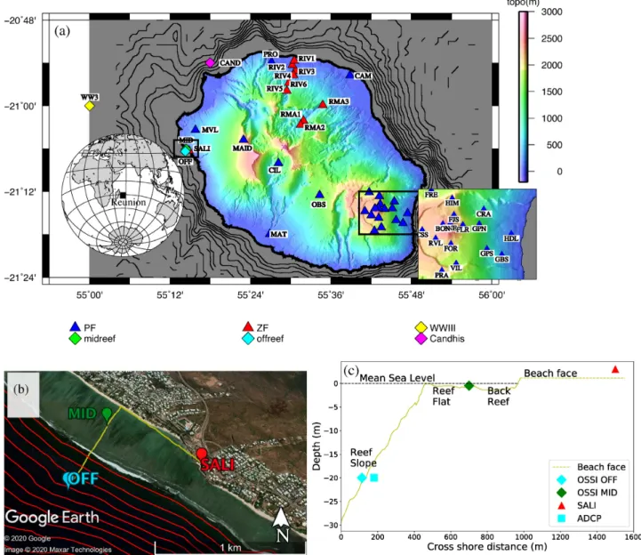
La R´eunion Island is located in the southwest (SW) Indian Ocean (Fig.1). It is affected by sporadic oceanic swells generated by trop-ical cyclones (occurring mainly during summer periods, i.e. from November to March) or by austral swell events (observed in austral winter, from April to October). Austral swells that reach La R´eunion Island are generated by distant storms in the Southern Indian Ocean at distance of 3000–4000 km (e.g. Davy et al.2015). Generated by strong winds and long fetches within strong atmospheric depres-sions circulating around Antarctica, the swells may take a few days to reach La R´eunion Island, where it may produce significant dam-age to the coastal infrastructures such as roads, houses, harbors, but also to the natural coral reef protecting part of the western coast of La R´eunion (e.g. Cordier et al.2012). Monitoring the swell activity
around the island and in the SW Indian Ocean is therefore of broad interest but is strongly limited by the little number of oceanographic sensors available. To extend the work of Davy et al. (2014,2015, 2016) and Barruol et al. (2016), we analyse the ocean-induced mi-croseismic noise recorded by terrestrial seismic stations installed on La R´eunion Island, and we combine those observables with in
situ ocean observations issued from two pressure sensors (OSSI,
Ocean Sensor Systems Inc.) deployed in the fringing reef and off shore, and an ADCP (Acoustic Doppler Current Profiler, Nortek Aquadopp Profiler) deployed off shore (Figs1b and c).
Microseisms have been long known to be generated by ocean gravity waves (e.g. Longuet-Higgins 1950) and can be recorded by seismic stations worldwide. The existence of two types of microseisms—the Primary and Secondary Microseisms (PM and SM, respectively), which differ from their dominant periods and
C
origins—is broadly accepted despite their origins and the involved processes are still actively studied (e.g. Ardhuin et al.2011,2015). PM are accepted to occur in coastal waters and concentrate the energy at the same period as the ocean swell, that is at periods∼10– 20 s (frequencies between 0.05 and 0.10 Hz). They are interpreted as the interaction between sloping seafloor and the approaching ocean waves (e.g. Hasselmann1963; Barruol et al.2006; Ardhuin
et al.2015). On the other hand, SM are accepted to be generated
within the ocean basins by the interaction of two swells of same periods propagating in opposite directions (e.g. Longuet-Higgins 1950), generating standing waves and vertical pressure variations across the water column, that excite seismic waves on the ocean bot-tom. SM therefore dominate at half the dominant swell periods, that is between∼3 and 10 s (frequencies between ∼0.10 and 0.33 Hz). SM sources have been located (1) in the open ocean where stand-ing waves are created by the interaction of two distant swells (e.g. Obrebski et al.2012), (2) in coastal regions where a swell reflected at the coast may interact with the incoming waves (e.g. Ardhuin
et al.2011; Stutzmann et al.2012; Bromirski et al.2013), gener-ating the so-called long period secondary microseism (LPSM) and (3) in a storm due to the interaction of two waves from opposite directions issued from the same system or waves issued from two different storms (e.g. Ardhuin et al. 2011; Obrebski et al.2013; Davy et al.2014).
In this study, we analyse a sequence of austral swells that hit La R´eunion Island between 13 March and 5 May 2017.
On land, we analyse the seismological data to determine the dom-inant frequency of the PM and SM using the power spectral density analysis that may provide a link to the swell peak period Tp; we
quantify the microseismic amplitudes by computing an hourly root mean square (RMS) in each frequency band that provides informa-tion on the local or distant significant wave height Hs(in the case of
the PM or SM band, respectively); we finally perform a polarization analysis to determine the dominant direction and strength of polar-ization of the recorded microseismic noise, that may indicate the wave peak direction Dp for the case of the PM band or the source
direction in the SM band.
At sea, oceanographic sensors were deployed during this period inside and outside the fringing reef along the west coast of La R´eunion Island: one sensor on the reef flat and two others on the reef external slope (Fig.1). Such in situ measurements allowed us to derive the local wave heights and periods from bottom pressure gauges and the swell direction from the ADCP sensor. We used those oceanographic observations, together with the land seismological data and the WaveWatch III (WWIII) swell models to establish relations between the observed and modelled swell parameters. One of the objectives of this work is indeed to establish the relationship between the land-recorded seismological PM amplitudes and the ocean-observed significant wave height (Hs, measured by the OSSI
pressure wave gauge) and to demonstrate that the PM can be used as a proxy of the Hs, and therefore, that a land seismometer can be used
as a well calibrated swell gauge. We also evaluate the accuracy of the modelled swell direction, height and period (respectively Dpm, Hsm
and Tpmparameters) derived from numerical models (WWIII) in the
west of La R´eunion Island by comparing them with the observed parameters. These approaches allow us to compute the transfer function relating the microseism amplitudes (in the PM and LPSM bands) and the wave height derived from the wave gauges and modelled from WWIII. We finally show that analysing distant SM sources can provide precursory information of the swells impacting La R´eunion Island.
2 S E I S M I C D AT A A N A LY S E S
This study uses data from the temporary deployment of 10 broad-band seismometers from the ‘Rivi`ere des Pluies’ network (Fontaine
et al.2015). Most of the stations deployed in the northern part of the island have been operated since 2016 and are installed along two hydrological basins in La R´eunion Island: the Rivi`ere des Pluies (RIV∗) and Rivi`ere du Mˆat (RMA∗). These stations were initially deployed to study the erosion and the sediment transport in the flooding rivers during cyclones (Gonzalez2019). The station SALI installed on the western shore of the island, in the very neighbour-hood of the fringing reef was deployed in February 2017 and is in appropriate location to study the swell seismic signature (Fig.1). We also used the data recorded by the permanent seismic stations (16 broad-band seismometers) of the Observatoire Volcanologique du Piton de la Fournaise (OVPF/IPGP). The seismic data are avail-able at the RESIF data portal (http://seismology.resif .f r) under the FDSN network code ZF and PF for the temporary and permanent stations, respectively. In this work, we analysed the microseismic noise recorded by these stations between 13 March and 5 May 2017, as oceanographic sensors (pressures gauges and ADCP) were deployed near to La R´eunion Island during this period (Fig.1).
Three methods are used to analyse the microseismic noise. (i) To constrain the swell period Tpin the neighbourhood of the
island, we calculate the seismological power spectral density (PSD) in the PM frequency band. To compute the PSD, we selected 1-hr data with 50 per cent overlap; then, each 1-hr time-series was divided into 13 segments with 75 per cent overlap between neighbouring segments, and later transformed into the time–frequency domain using the method of McNamara & Buland (2004). The obtained PSD was finally converted into decibels with respect to acceleration. To compute the daily average PSD into decibels with respect to acceleration as a function of the frequency, the sacpsd command from Herrmann (2013) was used.
(ii) To estimate the wave height Hs, we measured the hourly root
mean square (RMS) of the microseism amplitude. The information about the wave height that hit the coastal area can be found in the PM amplitude, while the SM amplitude gives us an insight about the wave height at the swell source location, that is within the storm where it is generated. To compute the RMS, we first converted the amplitude of the microseism into displacement (μm) by removing the instrument response. Then, we divided the data into 1-hr segments and applied a Butterworth bandpass filter with corner frequencies of 0.05 and 0.10 Hz for the PM and 0.10 and 0.33 Hz for the SM. The hourly RMS of the microseism amplitude were then computed from the filtered data. Finally, we determined the correlation coefficients between the microseism amplitude and the wave height using the Pearson method (Pearson1909). Estimating the significant wave height using seismic land station, have been successfully used before using different methods (e.g. Bromirski
et al.1999; Donne et al.2014).
(iii) To characterize the swell direction Dp, we performed a
polar-ization analysis using two methods: a complex polarpolar-ization analysis (e.g. Vidale1986) and a principal component analysis (e.g. Bar-ruol et al. 2006; Fontaine et al. 2009). Both methods provided comparable values, so we only present results from the second ap-proach. Analysing the polarization in the PM frequency band would give information regarding the swell direction before it breaks at the coastal area, while the polarization in the SM frequency band should give the information on the distant source (i.e. storm) backazimuth. Practically, we detrend and taper the three components (E–W, N–S
Figure 1. Location of the seismic stations and oceanographic instruments in La R´eunion Island. (a) Blue and red triangles show the permanent (OVPF/IPGP,
PF network) and temporary seismic network (Rivi`ere des Pluies, ZF network). Diamonds indicate the location of the wave gauge from the Candhis network installed in Le Port harbour (magenta) and the OSSI pressure instruments offshore (cyan) and in the lagoon (green). Yellow diamond shows the location of the WW3 model node used in this study. Bathymetry data is from D´el´egation Ifremer oc´ean Indien (2012) and 200 m isocontours are presented. (b) Green and cyan points indicate the pressure sensors located within the lagoon (MID, midreef) and the ADCP and pressure sensor deployed outside of the reef (OFF, offreef), respectively. SALI is the seismic station running on land close to the oceanographic instrumental transect. Yellow line shows the cross-section in subplot (c). The step of the bathymetric isocontour here is 5 m. (c) Schematic bathymetric cross-section illustrating the instrumental transect deployed from land (seismic station SALI) to the open ocean (ADCP+ pressure sensor deployed on the external slope of the reef), passing through the lagoon (pressure sensor).
and vertical) of the seismic waveform before converting them into ground velocity by removing the station response. For this step, we divided the data into hourly segments. For each segment, we ob-tained the eigenvalues and eigenvectors from which we derived the different parameters such as 0◦< backazimuth <360◦, and the co-efficient of polarization in the horizontal (0< CpH <1) and vertical (0< CpZ <1) planes (e.g. Barruol et al.2006). CpH or CpZ equal to 0 indicates a circular polarization in the corresponding plane, whereas a value of 1 indicates a perfectly rectilinear polarization. These different parameters were defined in Fontaine et al. (2009) and allow us to characterize the full 3-D ground motion, which helps us to locate the source of the microseism and to quantify the strength of polarization.
3 O C E A N I C WAV E D AT A A N A LY S E S
Three types of oceanic wave data were used in this study, two from local, in situ observations, and one from numerical modelling (Fig.1).
The first in situ data set was obtained from two ocean pressure sen-sors OSSI (Ocean Sensor Systems Inc) and from an ADCP (Nortek Aquadopp Profiler) deployed in the coastal area of La R´eunion Is-land from 13 March to 5 May 2017 (Fig.1). A first pressure sensor was installed inside the fringing reef at a depth of around 1 m (MID, Figs1b and c) and a second one on the reef external slope at a depth of 20 m (OFF, Figs1b and c). They were continuously recording the pressure induced by the sea surface variations at a sampling rate of 10 Hz. The pressure data were corrected from atmospheric mean
sea level pressure and non-hydrostatic pressure following linear wave theory (Hom-ma et al.1967). The tidal components were then removed from the computed water depth using a 2nd order Butter-worth lowpass filter with 6-hr cut-off frequency. Finally, a spectral analysis was performed on the detided signal to determine the wave power spectral density, from which an hourly time-series of wave height and period was extracted. To measure the wave propagation direction, the OFF pressure sensor was coupled with the ADCP, that recorded the pressure P and the two components U, V of the subsurface velocities variations at 2 Hz in burst mode of 1024 s for each hour. To compute the wave parameters, the PUV method was used, which involves a cross spectral analysis of the pressure P and the orbital velocities U and V (Pedersen2002; Sullivan et al.2006). The second in situ data set was obtained from the non-directional datawell wave buoy located at the ‘Rivi`ere des Galets’, a coastal station installed at a depth of 33 m, as part of the Candhis (Cen-tre d’Archivage National de Donn´ees de Houle In Situ) network (CAND, Fig.1). The data are freely available at the Candhis website (http://candhis.cetmef .developpement-durable.gouv.fr) from which one can retrieve hourly time-series of significant wave height (Hs)
and wave peak period (Tp).
Finally, the last data set used was an hourly forecast of wave pa-rameters issued from the 0.5◦resolution global wave model forecast distributed by the Pacific Islands Ocean Observing System (Pa-cIOOS, http://www.pacioos.hawaii.edu/waves/model-global) and configured in the School of Ocean and Earth Science and Technol-ogy (SOEST) at the University of Hawaii. These forecasts are based on the WaveWatch III model developed by the National Oceanic and Atmospheric Administration (NOAA) and National Centers for En-vironmental Prediction (NCEP). The hourly significant wave height (Hsm, with m subscript used for model), peak period (Tpm), peak
direction for sea state (Dpm) and for swell component only (Dpms)
were extracted at a node of the model located west of La R´eunion Island, at latitude 21◦S and longitude 55◦E (point WW3, Fig.1). The forecast parameters were used in this study because they have an hourly time step, which is similar to the observations and seismic data time steps. Also, as shown in Fig. S1, the data are comparable to the 3 hr hindcasts global wave model from IOWAGA Ifremer (Rascle & Ardhuin2013).
4 S P E C T R A L C H A R A C T E R I S T I C S O F M I C R O S E I S M S
The temporal evolution of the microseisms for station SALI derived from the PSD analysis between 13 March and 5 May 2017 is pre-sented in Figs2and S2. These figures indicate that both the PM and SM have a higher level of energy during the swell events, and that SM dominates the signal.
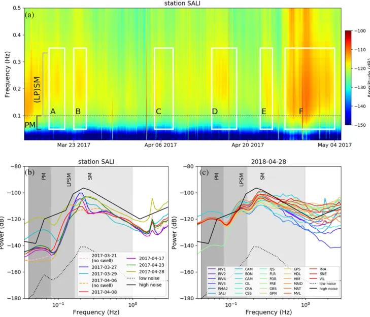
The daily average PSDs are presented in Fig.2(b) for the various individual swell events, selected by the white boxes on Fig.2(a) at station SALI, occurring between 13 March and 5 May 2017. Compared to a quiet period without any austral swell (indicated by the spectrum measured on 21 March and 6 April 2017, dashed colored lines Fig.2b), the increase of the microseismic noise during the occurrence of each swell is clearly observed in both the SM (up to 10 dB) and the PM bands (up to 30 dB) indicated by the different grey areas. Each swell event recorded at SALI has a clear signature in the PM band, the amplitude of which depends on the swell strength (Fig.2).
The very low level of noise in the PM band in the absence of swell is shown for two different days (21 March and 6 April 2017), but
the two corresponding daily spectra behave differently in the SM band. On April 6 (orange dashed line), the noise is very low in the SM band whereas on March 21 (pink dashed line), one can observe a peak of energy in the SM. This results from the fact that PM is known to be generated in shallow water, near coastal areas, due to a pressure variation at the bottom of the sea (e.g. Ardhuin et al. 2015) whereas the SM is sourced within storms at large distance in ocean basins. The high SM energy on March 21 likely indicates a distant storm that transmits the SM energy almost instantaneously at the seismic station, whereas the swell produced by this particular storm will reach the island only few days later. The presence of an individualized LPSM peak is observed for the April 28 event, which is the most energetic swell event visible on the spectrogram in Fig.2. It has twice the frequency of the PM, suggesting its local origin, due to interaction of the wave reflected from the coast with the incident swell. Such a process likely generates standing waves in the near-coastal region and provides energy in the LPSM band to the ocean floor.
Fig. 2(c) presents the PSD calculated for the individual swell event of 28 April 2017, but at the various seismic stations on La R´eunion Island. For this particular swell event, Fig.2(c) indicates the presence of clear PM, LPSM and SM peaks at all island stations. The homogeneous PM amplitudes indicate that the swell energy propagates well across the island. The two distinct peaks observed at∼0.15 Hz (LPSM) and ∼0.25 Hz (SM) suggest the presence of two source locations of secondary microseisms, with distinct dominant frequencies. Note that all of the stations recorded a com-parable amount of noise during the occurrence of this swell event. The exception being for station FOR where the PM is very low com-pared to the other stations, likely explained by a site effect causing attenuation close to the station.
5 C O M PA R I N G S W E L L D AT A A N D M I C R O S E I S M S A M P L I T U D E S
The wave data time-series are illustrated in Figs3and S3 for the coastal in situ observations and the swell modelled from WWIII. In general, the Hsm modelled at site WW3 (in red Fig.3a)
dis-plays a systematic higher amplitude compared to the actual coastal observations. Exception occurs on April 23 to 29 (Box F) during which the observed Hs offshore has the highest amplitude. This
observation could be associated to the fact that the global wave model (resolution 0.5◦) is relatively crude to represent coastal pro-cesses and that the waves modelled in the open ocean do not take into account refraction, diffraction and/or shoaling processes that occur at a local scale. In fact, the wave reflected from the coastal area (which produced the LPSM) attenuated rapidly and are likely to be weakly felt at the WWIII location (i.e. at latitude 21◦S and longitude 55◦E, WW3 node). However, despite these systematic amplitude differences, the time-series show very similar patterns with Hspeaks related to strong swell events occurring at the same
time in the observations and in the models.
An important insight shown in Fig.3(a) is the role of the reef as shore protector. The wave amplitudes are indeed reduced by a factor of∼10 when crossing the coral reef (see the 10 times smaller right vertical axis associated to the midreef Hsmeasurement as the pink
curve) while preserving very well the overall amplitude variations. This observation is in agreement with the tidal amplitude attenuation in the reef described by Cordier et al. (2012) in the same area, and indicates that the swell recorded inside the lagoon (midreef) is a very good proxy of the swell recorded further in the open ocean.
Figure 2. Power spectral density (PSD) of seismic noise converted into decibels relative to ground acceleration. (a) Spectrogram of the vertical component of
seismic station SALI from 13 March to 5 May 2017. White rectangles show the swell events we analysed in this work. The 10 s (0.10 Hz) period limit between PM and SM is marked by the horizontal dashed line. (b) Daily mean PSD of data recorded at station SALI (vertical component) during the occurrence of the austral swell events occurring between 13 March and 5 May 2017. The orange and pink dashed line indicates the PSD at this station during quiet days without swell. The source of the peak at 2 Hz observed at station SALI is not identified but is likely associated with anthropogenic activity in the site neighbourhood. (c) Mean PSD of the vertical components of the different stations in La R´eunion for the austral swell that occurred on 28 April 2017. For reference, the high and low noise models from Peterson (1993) are plotted in black continuous and dashed lines, respectively. Grey shadings indicate the frequency domains of PM, LPSM and SM.
Also, this shows the mechanical importance of a coral barrier to attenuate strong swell events and hence to avoid significant damage to coastal infrastructures.
Another observation from Fig.3(a) is that the amplitudes of the swell events are generally much smaller (except the event in box C) at the ‘Rivi`ere des Galets’ station (CAND) compared to those measured at the offshore coastal reef measurements (OFF). These differences likely suggest that the direction of propagation of the incident waves significantly affects how the waves impact the shore. The CAND station is indeed located 20 km north of the fringing reef area where the pressure measurements are performed. As the swells arrive from the south or the southwest, they likely experienced refraction and diffraction processes along the coast of the island, thus reducing their energy before being recorded at the
CAND station. Regarding the swell event of box C, its origin of propagation is slightly more westward, thus preventing the waves to be damped due to coastal processes before arriving at CAND station. Therefore, to better monitor the Austral swell activity in La R´eunion Island, it may be useful to have a buoy installed in the south.
The pattern of the PM and SM variations together with the ob-served Hsare presented in Figs3(b) and (c), respectively, and also
in Fig. S4. In general, for the austral swell events, the PM am-plitude and the observed Hs display very similar trends (Fig.3b).
However, a clear discrepancy between the two data set are ob-served at the early stage of the recordings (March 13–17). During this period, the PM has a high amplitude (also the SM, Fig.3c), while the observed Hs (in lagoon and offshore) remain low. We
Figure 3. (a) Significant wave height Hsrecorded by the different oceanographic instruments along the West coast of La R´eunion from 13 March to 5 May
2017. The offreef (blue line) and the midreef (magenta line) are derived from the pressure recorded off shore and in the lagoon, respectively. The Candhis (cyan) represents the wave gauge station located in Le Port (Fig.1). The significant wave height (Hs) from the NOAA WWIII model is shown in red and
extracted at node WW3 located on Fig.1. Note that the vertical axes are not at the same scale, for the offreef and Candhis stations (on the left) and for the midreef pressure sensor (on the right). (b) Time-series of the wave height measured in the lagoon (magenta) and primary microseisms (PM) amplitudes (green dots) from seismic station SALI, filtered in the 10–20 s period band. (c) Time-series of the offreef wave height Hs(blue line) and secondary microseisms (SM)
amplitudes (seismic data filtered in the 3–10 s period band), recorded at various seismic stations on La R´eunion Island (colored points). The high amplitude of the SM between March 13 and 16 is related to the ending phase of the tropical storm Fernando.
interpret these observations as induced by the tropical storm Fer-nando, which was active from March 6 to 15 in the SW Indian Ocean and which passed close to R´eunion Island on March 12 (http: //www.meteof rance.re/cyclone/saisons-passees). On March 13, the
storm was already south of the island and continued escaping south-ward. We suggest that this storm was likely still generating SM noise close to 10 s period (observed throughout the whole R´eunion island in both PM and SM bands), and a swell propagating towards the
different amplitudes from station to station. This indicates that the SM amplitude depends on the site effect near the station. A clear split in time between the elevated values of the SM and the local observed Hs(blue curves, Figs3c and S4) is also observed. The delay
times between the two parameters are proportional to the distance between the source location and the seismic station (discussed in Section 8). The recorded PM and SM amplitudes appear to depend not only on the strength of the storm that produced the swell and the distance between the source and the seismic station but also on a local site effect. For instance, the boxes A and B have similar SM amplitudes. However, the recorded Hscorresponding to box A is
relatively high compare to the Hsin box B (OFF Hs, Fig.3c).
6 C O R R E L AT I N G M I C R O S E I S M I C A M P L I T U D E S W I T H O B S E RV E D A N D M O D E L L E D WAV E
H E I G H T S — T R A N S F E R F U N C T I O N S
To determine the relationship between the local sea conditions and the microseismic noise, we correlate the RMS amplitude of the PM recorded at the seismic station SALI on land with the observed wave heights derived from the pressure sensors and the modelled wave heights from the WWIII model. Fig.3(b) shows the PM amplitude variation together with the swell amplitude observed inside the reef (midreef Hs). This plot clearly displays good correlations between
the two independent observables (except for the period when the tropical storm Fernando was still active), which we use below to determine transfer functions between microseismic noise amplitude and the wave height.
We focus here on the seismic station SALI which is the nearest to the oceanographic sensors (Fig.1) and which has the largest RMS amplitude during the observing period. To discuss the correlation between the microseismic noise and the significant wave height, we take as an example in Fig.4the Austral swell occurring between 23 April and 2 May 2017 (box F, Fig.3c). We chose this event, because of the presence of the LPSM and of the largest microseisms amplitudes. Figs4(a) to (h) compare the observed and modelled wave height and the RMS amplitudes in the PM (upper row in Fig.4) and in the LPSM (mid-row Fig.4) noise bands for seismic station SALI. Microseismic noise is compared to observed Hsinside the
reef (MID, midreef, Fig.4column I), outside the reef (OFF, offreef, Fig.4column II), northernmost off shore (at Candhis site, Fig.4 column III) and to the modelled Hsmat node WW3 (Fig.4column
IV). In these plots, each point represents an hourly measurement of the wave height and of the RMS microseismic noise amplitude.
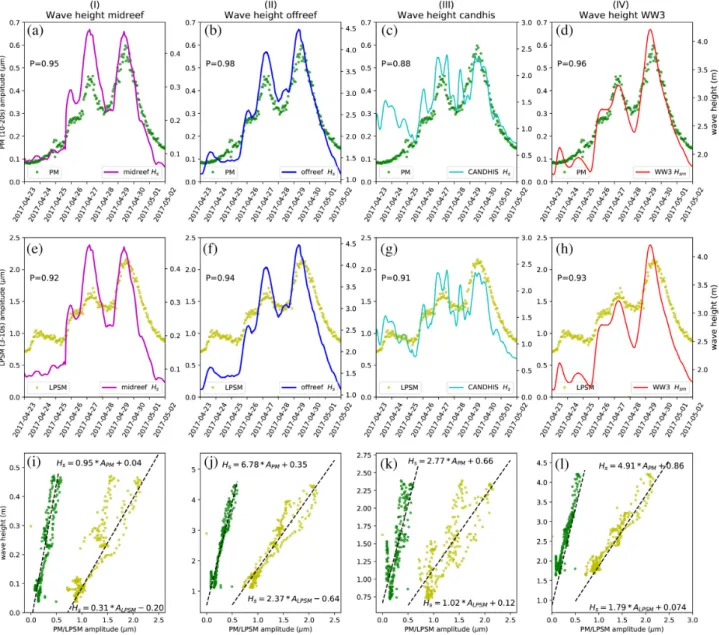
As shown in Fig.3(b), we observe a very good correlation be-tween the wave heights and the PM amplitude during the observing period. The amplitude of the PM correlates with both the observed significant wave height derived from the OSSI wave gauges (MID, midreef and OFF, offreef) and the WWIII model, with Pearson cor-relation coefficient>0.95 (Figs4a, b and d). These observations confirm that the PM relates to the local sea condition and is gen-erated in the very coastal region, as suggested by previous studies (e.g. Barruol et al.2006; Ardhuin et al. 2011). The correlation
wave height reduction is clearly visible by comparing the swell height measured offreef (29 April 2017, Fig.4b) and the maxi-mum of swell amplitude of 2.4 m observed further north at Candhis (Fig.4c).
The correlation between the amplitude of the LPSM and the sig-nificant wave heights for the different observations/model are plot-ted in Figs4(e)–(h). These figures show how well the LPSM and the wave heights correlate with Pearson coefficient >0.9. These observations strongly favour that the observed LPSM is gener-ated locally by the coastal reflected waves, which have been ob-served in other studies (e.g. Bromirski et al. 2005; Davy et al. 2016).
Figs4(a)–(h) indicate that the microseism amplitudes at station SALI in both the PM and LPSM frequency bands correlate well and are linearly proportional to the significant wave heights measured in the ocean or derived from the numerical model WWIII. This suggests that these two parameters can be linked using a simple linear equation. Therefore, we used a linear regression technique to establish the transfer function between these parameters, that is between the different measured or modelled wave heights and the PM or LPSM amplitudes. In total, we determine 8 transfer functions shown in Figs4(i)–(l). For each equation, the microseism amplitude and the wave height are inμm and in m, respectively. Note that dur-ing our linear regression, we used a thresholds values of 0.15 and 1.0
μm for the amplitude of the PM and LPSM, respectively. Therefore,
the transfer functions are only valid for the microseism amplitudes above these values, which represent the recorded amplitudes when there is no swell activity.
The transfer functions between the PM noise amplitude (in green, Fig.4) and the wave heights inside (MID, midreef) and outside (OFF, offreef) the reef, at the Candhis wave gauge and at the modelled WWIII point are Hs = 0.95∗APM+ 0.04, HS= 6.78∗APM+ 0.35, Hs = 2.77∗APM+ 0.66 and Hs = 4.91∗APM+ 0.86, respectively.
To validate these relations, we computed the wave height of the other swell events using the corresponding transfer function. Figs S5(a) to S5(d) show that the computed and the observed wave heights are comparable for the swell occurring between 21 and 25 March 2017 (box B, Fig.3c) and Figs S5(e) to S5(h) for the swell occurring from 7 to 11 April 2017 (box C, Fig. 3c). This suggests that these equations are valid for any austral swell events and demonstrate that one can derive a reasonable estimate of the wave height from the terrestrial observation of the amplitude of the primary microseisms. This confirms that the PM amplitude is a good proxy of the coastal wave height and that a well calibrated seismic station can become a terrestrial wave gauge that can be useful in the absence of direct wave gauge in the ocean, which is the case of La R´eunion Island. However, misfit between the observed and the computed wave heights are clearly observed for the 7–11 April swell event (box C, Fig.3c), for station CAND (Fig. S5g). As discussed in Sections 4 and 5, the misfit between the two data sets may be due to the presence of additional swell recorded at the Candhis buoy only, which was strongly dissipated and did not generate PM. The presence of the swell from other source(s) is confirmed by the fact that only during these periods (April 7–11, box C, Fig.3), Candhis station has the largest wave height amplitude.
Figure 4. RMS amplitude of the PM (top, a–d) and the LPSM (middle, e–h) together with the significant wave heights Hsfrom observations in the ocean (I,
midreef, II, offreef and III, Candhis station) and from the WWIII swell models extracted at node WW3 (IV) for the period 22 April to 2 May 2017. For each plot, the left axis represents the amplitudes of the microseisms (inμm) at station SALI and in the right axis the wave heights Hs(in m). P values indicate
the Pearson coefficient for the correlations. Bottom (i–l): Transfer functions between the significant wave height Hsand the hourly RMS amplitude of the PM
(green) and the LPSM (yellow). For each equation, APMand ALPSMstand for primary and long-period secondary microseisms amplitude, respectively.
7 D I R E C T I O N S A N D P E R I O D S O F S W E L L S D E D U C E D F R O M S E I S M I C N O I S E
We present in Fig.5(a) the hourly values of CpH and CpZ in the PM band, that is between 0.05 and 0.10 Hz, during the period 13 March and 5 May 2017 for station SALI, together with the Hs
observed inside the reef (MID, midreef). This figure indicates that prior to the swell arrival, most of the CpH are dispersed between 0.6 and 1.0, while CpZ varies between 0.8 and 1.0. Both of these values clearly focus above 0.95 during the occurrence of the wave events (marked by the boxes). Strong polarization in both vertical and horizontal planes, indicates a strong linear polarization of the ground motion, similar to a horizontally propagating compressional
P wave as described by Barruol et al. (2006) from near-shore seismic stations in French Polynesia islands.
The hourly measurements of the ground polarization azimuth at the coastal station SALI in the PM frequency band (0.05–0.10 Hz), together with the observed (ADCP Dp) and the modelled (WW3 Dpm
and Dpmsfor swell) azimuths are plotted in Fig.5(b). The azimuths
determined at the seismic station from polarization analysis (PM) are likely to be generated by the interaction of waves with the local bathymetry in the coastal area, and therefore, do not provide a measure of the direction of propagation of the swell at larger distance in the open ocean. In the following, we only referred to the azimuth values in the presence of swell activities (i.e. inside the boxes). Fig.5(b) indicates a fairly good agreement between the swell peak directions issued from the model (Dpms,∼N015◦E±5◦)
and the observed peak wave direction (Dp,∼N010◦E±10◦). It is
accepted that low frequency swells can propagate to longer distance with minimal energy loss (e.g. Ardhuin et al. 2009), therefore, the similarity between these two parameters (observed peak wave
(b)
Figure 5. (a) Polarization parameters CpH (red dots) and CpZ (blue dots) measured on an hourly base in the PM, together with the wave height Hsmeasured
in the lagoon (midreef, magenta line). Note that both polarization parameters (CpH and CpZ) are close to 1 for each swell event. (b) Plot of the polarization azimuths in the horizontal plane determined from the 3-D seismological data (green dots), and issued from oceanographic sensor ADCP (black dots) or from the WWIII model at the node WW3, swell peak wave direction (cyan dots) and wave peak direction for sea state (red dots).
direction nearshore and the modelled swells peak direction offshore) are not unexpected. The overall difference between the observed peak direction (Dp) and the modelled sea-state directions (Dpm) of
around∼25◦E±15◦ is due to the fact that the observed and the modelled peak wave directions do not relate to the same physical processes, since they are in coastal and deep water environments, respectively. The observations describe waves that have already been refracted, whereas the modelled waves have not been yet refracted and also include local wind-induced waves.
The azimuths measured from the seismic polarization analysis indicate a value equal to ∼N017◦E±8◦. The difference (∼10◦) between the observed (Dp) and the computed azimuth (PM) is
likely related to the swell progressive rotation when approaching the coast. As the swell interacts with relatively shallow bathymetry (half of the wavelength), the refraction process makes it progres-sively rotating and to finally propagate normal to the shoreline. Here, the estimated swell wavelength is around∼280 m (based on the modelled Tpm from the WWIII model), thus the waves likely
start refracting at a depth of∼140 m and continue until a depth of ∼14 m. This suggests that at the location of the ADCP (at ∼20 m depth, OFF location Fig.1), the swell has already begun to ro-tate and continues its rotation before breaking at the neighbouring reef crest.
A difference between the observed (∼N005◦E, Dp), the
mod-elled (∼N020◦E, Dpm) and the computed azimuths (∼N345◦E) is
observed for the swell in box F (i.e. April 28 to May 1). We propose that some of the reflected swells (from box E) propagated towards
the south and may have interacted with the incoming waves, pro-ducing simultaneously PM and LPSM peaks. These waves hit the coastal area at the south of the SALI station, resulting in the ob-tained azimuth ∼N345◦E. The difference between the observed swell direction (N005◦, Dp) and the modelled one (N025◦E, Dpm)
may suggest that the recorded directions by offreef (OFF) station (Dp) are partly related to the reflected swell from box E.
Alterna-tively, the ADCP (Dp) and the WWIII modelled (WW3, Dpm) could
have recorded different direction of the incident swells, as the waves propagate in many directions from the source.
The SM azimuths for the swells in boxes A, D and E (Figs6a and b), for SALI station, are estimated from seismic data polarization analyses to be N345◦E, N045◦E and N030◦E, respectively (Fig.6c). The azimuths for these swell events and for all seismic stations on La R´eunion Island are presented on the map in Fig.7. The com-puted azimuths in the secondary microseismic frequency band point towards to the storm where the swell is issued (Figs 6c and7). The observed and modelled azimuths of wave propagation (ADCP
Dp, WW3 Dpm) are however not comparable to the azimuths of the
source location (SM polarization) because the local oceanographic observations are influenced by the local coastal geometry. Conse-quently it is not surprising that the modelled azimuths ( Dpm) from
the WWIII model (at the point WW3 at latitude 21◦S and longitude 55◦E, Fig.1and for other nodes in the south of the Island Fig. S6) indicate the presence of the swells that have direction of prop-agation∼N010–030◦E and do not appear to change much despite different source locations during the observing period. Hence, the
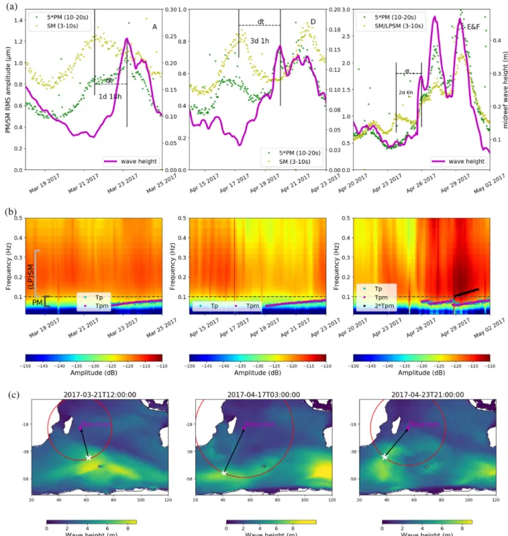
Figure 6. Examples of swell events, for station SALI. (a) Amplitude of the PM (green dots) and SM (yellow dots) and the midreef wave height (magenta line)
measured in the lagoon for time interval in boxes A, D, E and F (Fig.3c). Note that the amplitude of the PM is multiplied by a factor 5 to reach the same amplitude on the diagram as the SM. The dt shows the estimated delay time between the PM and SM. (b) Spectrograms of the vertical component of station SALI, together with the hourly swell frequency from the NOAA WWIII model (Tpmmagenta dots) and recorded offshore (cyan dots). Black dots indicate
(2∗Tpm) to show the good fit with the increase of energy in the LPSM. PM and SM frequency bands are separated by the horizontal dashed line. (c) Maps of
the Hs swell parameter issued from wave watch model WWIII on March 21 (left-hand panel), April 17 (middle panel) and April 23 (right-hand panel). Red circles show the distance between the seismic station in La R´eunion Island and the SM sources. White stars indicate the approximate location of the SM source, determined from its distance and its measured incoming azimuth. Black arrows indicate the SM azimuth determined from the seismic polarization analysis.
SM azimuths cannot be related to local oceanographic observations nor modelled values. However, as we discuss in section 8, the SM azimuths (combined with its amplitude) can be used as precursory information for swell arrivals.
The frequencies relative to the swell peak period (Tpm) from
WWIII (Fig.6, at the point WW3, latitude 21◦S and longitude 55◦E in Fig.1) and the observed peak period (Tp) by the offshore station
55˚12' 55˚24' 55˚36' 55˚48' 56˚00' −21˚24'
−21˚12'
SM:21−03−17 SM:17−04−17 SM:23−04−17
PF (Permanent stations) ZF (Temporary stations)
Figure 7. SM polarization azimuth measured at all seismic stations for the three swells presented in Fig.6(c). It shows a very homogeneous pattern of polarization in this frequency band. Bathymetry isocontours are displayed by step of 200 m.
Fig.6(b), for the swell events in boxes A, D, E and F. The observed (Tp) and modelled (Tpm) swells are similar and correlate well with
the PM periods (Fig.6b), suggesting that a coastal seismic station can be used to determine the swell’s dominant period.
During any swell event, a clear peak in the PM frequency band between 0.05 and 0.10 Hz is observed (Fig.2a), which corresponds to the swell frequency band. As presented in Section 4 and Figs2(b) and (c), the presence of the long period secondary microseism (LPSM) is observed for the April 28 swell event. The spectrum in Fig. 6(b) for box F confirms the presence of such LPSM, which displays frequencies twice of the PM. We interpret such LPSM as generated by interaction between the incoming and the reflected swells, which creates standing waves near to the coastal areas. This likely induces a pressure recorded by the wave gauge and trans-formed into seismic waves, recorded by the seismic station, which confirms the near coastal source of the LPSM issued from swell coastal reflection, as suggested from previous works (e.g. Bromirski
et al.2005; Ardhuin et al.2011). Bromirski et al. (2005) also sug-gested that the standing waves oscillate at twice the frequency of the incoming wave, such as the observed LPSM frequency here.
8 S M A S P R E C U R S O R S O F S T R O N G S W E L L S I M PA C T I N G L A R ´E U N I O N I S L A N D
During the observing period (March 13 to May 5), SM often display a peak in amplitude preceding the actual arrival time of the Hs
peak measured by the ocean sensor (Fig.3c) and by seismic PM amplitude (Fig.3b). In several cases, swells hit the coast (peak in the offreef Hs, Fig.3c)∼1–3 d after the SM is recorded on-land at the seismic stations (boxes A, B, D and E, Figs3c and 6a). Exception is observed during the period April 8–13 (box C, Fig.3), while PM arrived a few hours before the SM, likely indicating the absence of causal relationship between them. Also, for box F, the
(LP)SM and PM (Fig.6a) were recorded at the same time favouring a (LP)SM source located close to the coast. Note also the presence of high SM amplitude (also PM amplitude but with low Hs) without
any Hs followed, at the beginning of the recording (March 13–
18). As discussed in Section 5, we interpret that these observations are related to the final stage of the tropical storm Fernando. On March 13, the cyclone was already at the south of the island and continued to propagate southward and was likely generating a swell propagating towards the south with a dominant period of 10 s. It is therefore likely that the PM recorded by the stations SALI had a distant origin and was not generated by a local swell, explaining thus the low Hs. Some examples of swell activities (boxes A, D, E
and F in Fig.3c) are presented in the following and are illustrated in Fig.6.
Fig.6(a) shows in greater detail that the maximum in SM am-plitude (3–10 s, in yellow) measured at station SALI arrives before the PM peak (green dots) and the wave height peak (in the midreef station, in magenta). This can be explained by the signals associated with the SM travelling as a seismic wave in the solid Earth, whereas the PM is generated by ocean waves that travel across the ocean at much slower velocity. The SM is indeed generated within the active storm by the interaction of two swells of similar periods and can be recorded almost instantaneously at a seismic station, with delay time depending on the distance between the source and the seismic station. Assuming that the surface waves that dominate the SM propagate at∼3 km s–1, they reach the station located thousands
km away within few minutes. In the meantime, the swell generated by the same storm is accepted to travel at a velocity between 40 and 60 km hr–1 depending on the wave period. At 50 km hr–1for
instance, the swell may cross 1000 km of the ocean within 20 hr and for a distance of 4000 km (from La R´eunion to a storm centre) will require more than 3 d of travel. This results in the observed delay times (dt in Fig.6a) between the SM and the PM and/or Hs. The secondary microseisms can arrive simultaneously or shortly after the PM in case of near coastal sources of LPSM (box F, Fig.6a)
or it may take few days (boxes A, B, D and E) for distant sources. Fig.6(a) shows that for box A, the SM peak was estimated to be recorded 1 d and 18 hr before the PM peak, while for the box D, the time difference between the PM and the SM was estimated to be 3 d and 1 hr, suggesting a more distant storm. For box E, the PM peak arrived 2 d and 6 hr after the SM. The reflected swells from box E interfere with an incoming swell likely resulting in a near-coastal area source for the secondary microseisms (i.e. presence of LPSM). Thus, for box F (swell impacting La R´eunion on 26 April 2017) the PM and SM (i.e. LPSM) arrived at the same time.
To estimate the SM source location, we first estimate its distance from the delay time between the PM and SM and the group velocity
U(f), such as d= U(f)∗dt (e.g. Chevrot et al.2007), in which dt is the delay time (between PM and SM) and U(f)= 3.6∗g/(4∗π∗f), with g the gravitational acceleration (9.8 m2s–1), and f is the wave
frequency that can be determined from the slope of the PM (Fig.6b). The constant 3.6 is used to convert the velocity into km hr–1. Fig.6(c)
plots the possible SM source locations on the red circles, for each of the swells indicated in boxes A, D and E. Secondly, by performing a polarization analysis, we determine the incoming direction (az-imuth) of the secondary microseisms. For station SALI, we obtained an azimuth of N345◦E, N030◦E and N040◦E for boxes A, D and E, respectively (black arrows Fig.6c). For each event, the intersec-tion of the azimuth of incoming noise derived from the polarizaintersec-tion analysis with the distance circle provides a rough approximation of the SM source location (white stars). We observe that in the three cases (boxes A, D and E), the white stars are in areas of maximum
Hsparameters (yellow colours), indicating the SM source location
is consistent with the swell activity (WWIII model) and that the maximum noise is generated in areas of maximum wave heights within the storms. We performed a polarization analysis for all sta-tions in Fig.1(a) and the computed azimuth for those stations, for the three swells (boxes A, D and E), are presented in Fig.7. This Figure shows that all the stations consistently pointed to approxi-mately towards the same sources: N345◦E (box A), N030◦E (box D) and N040◦E (box E).
This simple analysis indicates first the feasibility of combining the delay time between the seismologically derived PM and SM peaks and the polarization analysis to locate the SM noise source. Secondly, this analysis also demonstrates that a continuous moni-toring of the SM amplitude could be used to determine precursory information of the swell height that might impact the island few days later. Unfortunately, the SM data alone are not sufficient to predict the arrival time and the amplitude of the swell to hit the island. In order to carry out the prediction of the swell, the SM in-formation could be combined with satellite data or wave forecasting models. Knowing the areas of the maximum Hs parameters in the
oceans, one can estimate the arrival time of the PM and its strength and therefore, anticipate the impact of strong swell events on the island. The use of the SM could improve the accuracy of the existing models of swell forecasting (e.g.https://www.surf -f orecast.com/) around the La R´eunion Island. More generally, microseismic noise analysis will not only increase the number of ocean observations but will also be very useful in validating ocean wave models worldwide (e.g. Stopa et al.2019).
9 C O N C L U S I O N S
This study shows that terrestrial seismic stations may represent al-ternative tools to improve swell observations, especially in regions of limited number of oceanographic sensors and in regions where
cyclones and storms may render surface buoy deployments very hazardous. We demonstrate the reliability of using the microseis-mic noise recorded by land seismicroseis-mic stations as a swell proxy. We derive the significant wave height and period parameters (Hs and
Tp) together with the wave direction (Dp) from pressure gauges and
Acoustic Doppler Current Profiler (ADCP), respectively. These in-struments were deployed on the ocean bottom in La R´eunion near-coastal areas and were operated in March–May 2017. The swell periods Tpwere also retrieved from spectral analyses of the
micro-seismic noise. Our results show that the swells measured on both sides of the reef display similar variations, but with an amplitude outside the reef about ten times higher than that inside, evidencing a strong reduction of the swell strength when crossing the reef crest, while preserving its frequency content. From the high correlation between the Hsand the primary microseisms (PM, 0.05-0.10 Hz)
amplitudes (correlation coefficients>0.92), we established linear transfer functions between the two data sets that can be used for quantifying swell height from terrestrial seismic observations. A good correlation between the long-period secondary microseisms (LPSM, 0.10–0.15 Hz) and Hs is also observed in case of
near-coastal source of microseisms. The secondary microseisms (SM, 0.10–0.33 Hz) that develop within the storm at several thousands of km and that propagate as seismic waves in the solid Earth arrive∼1– 3 d before the swell hits the coast of La R´eunion Island, indicating that SM may represent good precursors of an extreme swell event. We estimated the location of the SM source from the polarization analysis and the delay time between the arrival times of the PM and SM, which fits well with the WWIII wave height model. We there-fore propose that continuous monitoring of SM may provide good precursory information for strong swells reaching the island, that can also be used to validate the existing forecasting global model around the island.
A C K N O W L E D G E M E N T S
We acknowledge the French INSU-RESIF/SISMOB instrumen-tal pool for providing five stations deployed in the ‘Rivi`ere des Pluies’ network. The data are archived at RESIF data centre (http://seismology.resif .f r) and will be available in 2022, http: //dx.doi.org/10.15778/RESIF.ZF2015. We are thankful to M´et´eo-France and the French ‘Minist`ere de la D´efense’ to kindly provide access to their site in ‘La Saline’. We are very grateful to the OVPF (Observatoire Volcanologique du Piton de la Fournaise) and IPGP colleagues who maintain the PF seismic stations and for the easy access and the quality of their data. We appreciate the help of E. Delcher and A. Gonzalez during the Rivi`ere des Pluies field-works. E. Rindraharisaona and the oceanographic instruments and deployments were funded by the ReNovRisk project supported by the FEDER (Fond Europ´een de D´eveloppement R´egional), R´egion R´eunion, Etat Franc¸ais CPER (Contrat de Plan Etat R´egion) and European Community. Thanks to the University of La R´eunion and the Laboratoire Geosciences R´eunion for their supports. Part of the wave data used in this study were collected during the CAL-HYCO research program (2015–2017) funded by R´egion R´eunion. We thank Anya M. Reading and Laura Ermert for providing con-structive comments and Editor Martin Schimmel for additional care-ful reading of the paper. This is IPGP contribution number 4114.
R E F E R E N C E S
Ardhuin, F., Mari´e, L., Rascle, N., Forget, P. & Roland, A., 2009. Observation and estimation of Lagrangian, Stokes and Eulerian currents induced by wind and waves at the sea surface, J. Phys. Oceanogr., 39, 2820–2838.
K., 2016. Monitoring Austral and cyclonic swells in the “Iles Eparses”(Mozambique channel) from microseismic noise, Acta
Oeco-logica, 72, 120–128, doi:10.1016/j.actao.2015.10.015.
Barruol, G., Reymond, D., Fontaine, F.R., Hyvernaud, O., Maurer, V. & Maamaatuaiahutapu, K., 2006. Characterizing swells in the southern Pa-cific from seismic and infrasonic noise analyses, Geophys. J. Int., 164(3), 516–542, doi:10.1111/J.1365-246X.2006.02871.x.
Bromirski, P.D., Duennebier, F.K. & Stephen, R.A., 2005. Mid-ocean micro-seisms, Geochem., Geophys., Geosys., 6(4), doi:10.1029/2004GC000768. Bromirski, P.D., Flick, R.E. & Graham, N., 1999. Ocean wave height deter-mined from inland seismometer data: implications for investigating wave climate changes in the NE Pacific, J. geophys. Res., 104(C9), 20 753– 20 766.
Bromirski, P.D., Stephen, R.A. & Gerstoft, P., 2013. Are deep-ocean-generated surface-wave microseisms observed on land?, J. geophys. Res.,
118(7), 3610–3629.
Chevrot, S., Sylvander, M., Benahmed, S., Ponsolles, C., Lefevre, J. & Paradis, D., 2007. Source locations of secondary microseisms in Western Europe: evidence for both coastal and pelagic sources, J. geophys. Res.,
112(B11), doi:10.1029/2007JB005059.
Cordier, E., Poizot, E. & Mear, Y., 2012. Swell impact on reef sedimentary processes: a case study of the La R´eunion fringing reef, Sedimentology,
59(7), 2004–2023.
Davy, C., Barruol, G., Fontaine, F.R. & Cordier, E., 2016. Analyses of extreme swell events on La R´eunion Island from microseismic noise,
Geophys. J. Int., 207(3), 1767–1782, doi:10.1093/gji/ggw365.
Davy, C., Barruol, G., Fontaine, F.R., Sigloch, K. & Stutzmann, E., 2014. Tracking major storms from microseismic and hydroacoustic ob-servations on the seafloor, Geophys. Res. Lett., 41(24), 8825–8831, doi:10.1002/2014GL062319.
Davy, C., Stutzmann, E., Barruol, G., Fontaine, F.R. & Schimmel, M., 2015. Sources of secondary microseisms in the Indian ocean, Geophys. J. Int.,
202(2), 1180–1189, doi:10.1093/gji/ggv221.
D´el´egation Ifremer oc´ean Indien, 2012, BATHYMETRIE : MNT Hydrorun `a 100m pour les 6 mod`eles de rang 3 autour de l’ˆıle de La R´eunion,https: //sextant.if remer.fr/record/70a263ff -8095-4dcd-9d82-16badd19453d/. Donne, S., Nicolau, M., Bean, C. & O’Neill, M., 2014. Wave height
quan-tification using land based seismic data with grammatical evolution , in
Proceedings of the 2014 IEEE Congress on Evolutionary Computation (CEC), pp. 2909–2916, IEEE.
Fontaine, F.R., Barruol, G., Kennett, B.L., Bokelmann, G.H.R. & Reymond, D., 2009. Upper mantle anisotropy beneath Australia and Tahiti from P-wave polarization: implications for real-time earthquake location, J.
geophys. Res., 114(B3), doi:10.1029/2008JB005709.
Fontaine, F.R., Barruol, G. & Gonzalez, A., 2015. Rivi`ere des Pluies Project, La R´eunion Island, 2015-2018 2015-2018; RESIF - R´eseau Sismologique et g´eod´esique Franc¸ais. http://dx. doi.org/10.15778/RESIF.ZF2015 . Gonzalez, A., 2019, Suivi sismologique de l’impact des cyclones sur
la charge de fond de la Rivi`ere des Pluies et de la Rivi`ere du Mˆat `a La R´eunion. PhD thesis, Universit´e de La R´eunion, Saint-Denis, 164 pp.
Hasselmann, K., 1963. A statistical analysis of the generation of micro-seisms, Rev. Geophys., 1(2), 177–210.
Herrmann, R.B., 2013. Computer programs in seismology: An evolving tool for instruction and research, Seismol. Res. Lett., 84(6), 1081–1088. Hom-ma, M., Horikawa, K. & Komori, S., 1967. Response characteristics
of underwater wave gauge, Coast. Eng. J., 9(1), 45–54.
Longuet-Higgins, M.S., 1950. A theory of the origin of microseisms, Phil.
Trans. R. Soc. Lond., A, 243(857), 1–35.
modeling of oceanic noise sources, J. geophys. Res., 118(8), 4312–4324. Pearson, K., 1909. On a new method of determining correlation between a measured character a, and a character b, of which only the percentage of cases wherein b exceeds (or falls short of) a given intensity is recorded for each grade of a, Biometrika, 7(1/2), 96–105.
Pedersen, T., 2002. Wave measurements using the PUV method, Technical Report, Nortek Group, 15 p.
Peterson, J., 1993. Observations and modeling of seismic background noise, US Geological Survey, pp. 93–322.
Rascle, N. & Ardhuin, F., 2013. A global wave parameter database for geophysical applications. Part 2: model validation with improved source term parameterization, Ocean Model., 70, 174–188.
Stopa, J., Ardhuin, F., Stutzmann, E. & Lecocq, T., 2019. Sea state trends and variability: consistency between models, altimeters, buoys, and seismic data (1979-2016), J. geophys. Res., 124(6), 3923–3940.
Stutzmann, E., Ardhuin, F., Schimmel, M., Mangeney, A. & Patau, G., 2012. Modelling long-term seismic noise in various environments, Geophys. J.
Int., 191(2), 707–722.
Sullivan, C., Warner, J., Martin, M., Lightsom, F., Voulgaris, G. & Work, P., 2006, Wave Data Processing Toolbox Manual, Open-File Report 2005-1211, USGS.
Vidale, J.E., 1986. Complex polarization analysis of particle motion, Bull.
seism. Soc. Am., 76(5), 1393–1405.
S U P P O RT I N G I N F O R M AT I O N
Supplementary data are available atGJ Ionline.
sm Assessing Swell Reunion.pdf
Figure S1 Comparison between the Haiwaii/NOAA/NCEP and
IFREMER wave models, (a) wave height Hs, (b) swell frequncy
(period Tp) and (c) swell direction Tp.
Figure S2 Top panel: spectrograms of vertical component from 13
March to 5 May 2017 at station SALI. Rectangles show the swell that we analysed/discussed in this work (same as Fig.2a). Bottom panel: time evolution of the PM (blue) and SM (red).
Figure S3 (a) Continuous line shows the significant wave height
for the different oceanography stations (same as Fig.3a). (b) Plot of the offreef versus midreef amplitudes showing the attenuation of the wave when crossed the reef.
Figure S4 PM (top panel) and SM (bottom panel) RMS amplitude
for all seismic stations versus significant wave heights in the Lagoon (midreef) and offshore (offreef).
Figure S5 PM RMS amplitude (green dots) for SALI station versus
wave heights for swells in boxes A and C (Fig.3). The Observed wave heights for offreef (blue), midreef (magenta), Candhis (cyan) and from modelled WWIII (red) are plotted in continuous lines here. The dashed lines indicate the estimated wave heights using the transfer function from Section 6 and Fig.4.
Figure S6 Plot of the polarization azimuths in the horizontal plane
determined from the 3-D seismological data (green dots), and issued from oceanography sensor ADCP (black dots) or from the WWIII model at the different nodes S21◦E55◦(red dots), S21.5◦E55◦(cyan dots), S21.5◦E55.5◦(magenta dots) and S21.5◦E56◦(yellow dots). In general, the WWIII model at different nodes show a comparable direction.