OATAO is an open access repository that collects the work of Toulouse
researchers and makes it freely available over the web where possible
Any correspondence concerning this service should be sent
to the repository administrator:
[email protected]
This is a author’s version published in:
http://oatao.univ-toulouse.fr/25645
To cite this version:
Rida, Zeinab and Cazin, Sébastien and Lamadie, Fabrice and
Dherbecourt, Diane and Charton, Sophie and Climent, Éric
Experimental investigation of mixing efficiency in
particle‑laden Taylor–Couette flows. (2019) Experiments in
Fluids, 60 (61). 1-13. ISSN 0723-4864.
Official URL:
https://doi.org/10.1007/s00348-019-2710-9
Experimental investigation of mixing efficiency in particle‑laden
Taylor–Couette flows
Zeinab Rida1 · Sébastien Cazin1 · Fabrice Lamadie2 · Diane Dherbécourt2 · Sophie Charton2 · Eric Climent1
Abstract
This paper reports on original experimental data of mixing in two-phase Taylor–Couette flows. Neutrally buoyant particles with increasing volume concentration enhance significantly mixing of a passive tracer injected within the gap between two concentric cylinders. Mixing efficiency is measured by planar laser-induced fluorescence coupled to particle image velocime-try to detect the Taylor vortices. To achieve reliable experimental data, index matching of both phases is used together with a second PLIF channel. From this second PLIF measurements, dynamic masks of the particle positions in the laser sheet are determined and used to calculate accurately the segregation index of the tracer concentration. Experimental techniques have been thoroughly validated through calibration and robustness tests. Three particle sizes were considered, in two different flow regimes to emphasize their specific roles on the mixing dynamics.
List of symbols Variables
A Area of pixels with value 1 (–)
C Concentration (–)
C Mean concentration (–)
e Gap width (m)
H Height (m)
I Segregation index (u.a.)
m Azimuthal wavenumber (–)
n Refraction index (–)
R
d Initial decay rate (–)
Re Stator radius (m) R i Rotor radius (m) Re𝛺 Reynolds number (–) r Radial coordinate (m) Tc Rotational period (s) t 1∕2 , t90 , t99 Mixing times (s)
𝛤 = H∕e Aspect ratio (–)
𝛤 Mean shear rate ( s−1)
𝜆 Axial wavelength (–)
𝜈 Kinematic viscosity ( m2s−1)
𝛺 Rotation rate ( rad s−1)
𝜌 Density ( kg m−3) 𝜎 Standard deviation (–) 𝜎2 Variance (–) Abbreviations DMSO Dimethyl-sulfoxide KSCN Thiocyanate of potassium
PIV Particle image velocimetry
PLIF Planar laser-induced fluorescence
sCMOS Camera (scientific complementary metal
oxide semi-conductor)
SVF Spiral vortex flow
TVF Taylor vortex flow
WVF Wavy vortex flow
Subscripts
c Critical
i Relative to the rotor
e Relative to the stator
* Eric Climent [email protected] Zeinab Rida [email protected] Sébastien Cazin [email protected] Fabrice Lamadie [email protected] Diane Dherbécourt [email protected] Sophie Charton [email protected]
1 Institut de Mécanique des Fluides de Toulouse (IMFT),
Université de Toulouse, CNRS, Toulouse, France
2 CEA, DEN, MAR, DMRC, SA2I,
0 Relative to the origin value
rz In the vertical visualization plane
1 Introduction
Solvent extraction process is generally carried out in indus-trial counter-current flow contactors, such as agitated or pulsed columns which typical size can be as large as 1 m diameter with throughput as high as several hundreds of cubic meters per hour. However, R&D devices dedicated to new processes (e.g., test of new solvent, assessment of impurities effects, etc.) require small-scale contactors, demanding reduced amount of reagents, mainly for economi-cal and environmental issues. Typieconomi-cally, the inner diameter of the smallest lab-scale columns ranges from 30 mm (for Kühni-type columns) to 15 mm (for pulsed columns), with a nominal throughput of few liters per hour. Taylor–Cou-ette flow columns have shown very high extraction
perfor-mances (Davis and Weber 1960; Lanoë 2002). The annular
gap between the two concentric cylinders is only a few mm wide, while typical flow rates are as low as few hundreds of milliliters per hour. The efficiency of such miniature Taylor–Couette columns is mainly attributed to the high shear prevailing between the contra-rotating vortices that enable significant increase of the interfacial drop area for mass transfer. Moreover, thanks to low axial dispersion
pre-vailing in Taylor–Vortex flow (Kataoka et al. 1975, 1977;
Kataoka and Takigawa 1981), the height of the column can
be reduced by a factor 10 while achieving the same separa-tion performances as large scale industrial columns. One important feature of such columns is their low axial diffusion coefficient. The latter accounts for all coupling phenomena between hydrodynamics and mass transfer (e.g., molecular diffusion, local velocity gradients, eddies, etc.). Wilkinson
and Dutcher (2018) have studied experimentally axial mass
transport behaviour over two orders of magnitude of Reyn-olds number in a Taylor–Couette device. Therefore, mix-ing prediction is a determinant point for the design of such industrial processes.
In this aim, (Nemri et al. 2013) studied axial
disper-sion in a Poiseuille–Taylor–Couette flow based on numeri-cal simulations and measurements of dye residence time distribution. A significant effect of the flow regime was evidenced on mixing due to the successive flow bifurca-tions. These results are consistent with previously reported experimental and numerical studies (Campero and Vigil
1997; Desmet et al. 1996a, b; Kataoka et al. 1975; Tam
and Swinney 1987; Rudman 1998). Simultaneous
par-ticle image velocimetry (PIV) and planar laser-induced
fluorescence (PLIF) measurements (Nemri et al. 2014,
2016) were combined to highlight the enhanced chaotic
advection in the mixing process for wavy regimes. The
purpose of the present study is to measure the specific role of a dispersed phase on the progressive mixing of dye under similar flow conditions. Solid particles will be used to model small spherical droplets encountered in extrac-tion columns. Mixing is expected to be enhanced under two-phase flow configurations. Using LIF measurements,
Metzger et al. (2013) have analyzed individual particle
tra-jectories in a cylindrical Couette flow. They measured an additional contribution to the rate of heat transfer across the cell due to non-Brownian neutrally buoyant particles. A significant increase of the effective thermal diffusivity was evidenced for low Reynolds shear flow. This effect was attenuated for dense suspension (40% volume frac-tion), as the steric interaction impedes the chaotic motion
of the particles. Souzy et al. (2017) further investigated the
mechanisms responsible for this shear-induced mixing in linear shear flow. From instantaneous 2D velocity fields obtained by high-resolution PIV, they examined stretching intensity in a suspension of monodisperse PMMA particles (volume fraction ranging from 20 to 55%). The authors showed that mixing is not only increased by the particles, but that it also follows a different evolution compared to single-phase flow (the usual linear stretching law turns to an exponential behaviour). In a recent preliminary study, similar mixing enhancement induced by particles was
observed by Dherbécourt et al. (2016) with neutrally
buoy-ant particles in Taylor–Couette flows. The aim of the pre-sent study is to measure mixing efficiency for systematic variations of particle size and concentration. Following
(Nemri et al. 2014), coupled PIV and PLIV measurements
are implemented to measure mixing in steady and unsteady Taylor–Couette flow regimes. However, in the case of sus-pension flow, an additional issue arises. Indeed, due to the random spatial distribution of particles, an additional PLIF channel is required to detect the particle boundaries thus allowing appropriate correction of the dye concentration fields.
The paper is organized as follows. The original setup, based on three synchronized optical channels (one PIV
and two PLIF) is described in Sect. 2. It is used to study
mixing mechanisms in particle-laden Taylor–Couette flows. Thanks to thoroughly validated post-processing
procedures (in Sect. 2.4), reliable data on the mixing
effi-ciency in two-phase Taylor–Couette flows is obtained. The experimental data showing the specific effect of the par-ticulate phase on the enhancement of mixing are discussed
in Sect. 3. Conclusions are drawn in the final section of
2 Materials and improvement
of experimental techniques
2.1 Experimental setup and flow regimes
The Taylor–Couette configuration consists in a fluid flow driven by two coaxial circular cylinders which rotate independently along the vertical direction. In this study, the borosilicate outer cylinder, i.e., the stator, of radius
R
e is kept fixed, while the inner polycarbonate cylinder,
i.e., the rotor, of radius Ri rotates with a controlled
veloc-ity, 𝛺 . A visualization box made of optical quality glass (1 cm thick) filled with liquid of the same refractive index as borosilicate, is placed on the stator to reduce optical
deformations (see Fig. 1). Since Taylor–Couette flow is
very sensitive to initial and flow history (Coles 1965), a
motor is connected to a ramp generator for fine
veloc-ity and acceleration tuning (resolution of 8.10−4 rad/s) to
ensure experimental reproducibility.
The geometric characteristics of the experimental device
are presented in Table 1.
2.1.1 Determination of flow regimes
The Reynolds number Re𝛺 (Eq. 1) is a dimensionless quantity
which compares the relative magnitude of inertia and viscous effects. It is convenient to identify the successive transitions
between different flow regimes in Fig. 2. The Reynolds
num-bers of transition between different regimes depend on the
geometry of the column (Esser and Grossmann 1996; Dutcher
and Muller 2009):
(1)
Re𝛺 = 𝛺Rie
𝜈 ,
Fig. 1 Experimental device: 1. rotor; 2. sampling ports; 3. motor; 4. visualization box; 5. stator
Table 1 Geometry of the device
Stator radius ( Re) 35 mm
Rotor radius ( Ri) 24 mm
Gap width (e) 11 mm
Radius ratio ( 𝜂 = Re∕Ri) 0.687
Height (H) 640 mm
Aspect ratio ( 𝛤 = H∕e) 58
Rotation rate 0.1–20 rad/s
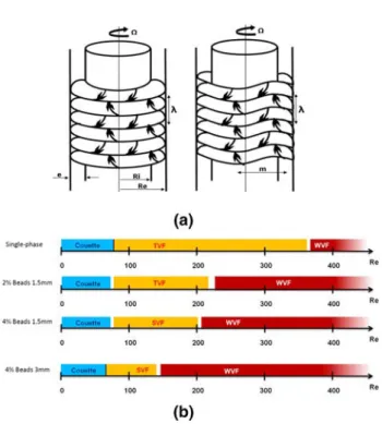
Fig. 2 a Visualization of the flow regimes by increasing the rotation
rate [TVF (left), WVF (right)], and their corresponding axial wave-lengths 𝜆 . b Particles effect on the flow transitions. From top to bot-tom: single-phase flow configuration, Ri∕Re= 0.687 and two-phase
where for two-phase flows, 𝜈 is the viscosity of the particu-late suspension which ranges from the fluid viscosity for a very dilute regime, to a viscosity increase of 24% when the particle concentration is 8% based on Eilers’ correlation.
When the rotation rate, 𝛺 , increases, successive insta-bilities occur (characterized by the formation and oscilla-tion of vortices). Considering single-phase flow, Andereck
et al. (1985) elaborated a detailed phase diagram composed
of the 26 possible stable configurations observed when the two cylinders are allowed to rotate. When the outer cylin-der is at rest, only five regimes are commonly observed for single-phase flows. The Couette regime, which is the first regime that appears at low Reynolds, is laminar and steady (its velocity profile is provided in standard textbooks). The fluid flow has a single velocity component along the azi-muthal direction, and depends only on the radial distance r from the axis of rotation. When the rotation rate increases, Taylor Vortex Flow regime (TVF) appears. It results from a centrifugal instability that leads to the formation of toroidal vortices in the flow direction. These vortices are perpendicu-lar to the axis of rotation and are organized by pair (contra-rotative vortices). The flow in TVF regime is still axisym-metric and steady. For a given Reynolds number Re, the flow configuration is characterized by its axial wavelength,
𝜆 , that represents the length of a pair of vortices (typically 𝜆
is slightly larger than 2e, where e is the gap width between the two cylinders).
By further increasing the rotation velocity, the vortices start to deform and undulate periodically. This corresponds to the Wavy Vortex Flow (WVF) regime which is fully tri-dimensional and unsteady, characterized by the axial wave-length, 𝜆 , and the azimuthal wave-number m, as shown in
Fig. 2a. At higher Reynolds numbers, the vortices deform
and a progressive transition to Turbulent Taylor Vortex Flow regime occurs.
A usual procedure was used to determine the transition between the flow regimes in the two-phase flow configura-tions. The liquid phase was seeded with micrometric inert particles of mica (4–32 μm), known as kalliroscope flakes. In presence of incident light, the kalliroscope reflects light yielding streamlines to become visible. This method allows a direct measurement of the axial wavelength of the flow regime. Under our experimental conditions, transitions between regimes for single-phase flow were determined by
Nemri et al. (2013). They are summarized in Fig. 2b which
also shows the flow regimes we identified for the two-phase configurations in which mixing will be investigated. In our experiments, due to the presence of particles, an additional regime has been observed which is not expected in a single-phase flow, where the outer cylinder is at rest. This Spiral Vortex Flow regime (SVF) was indeed only observed for single-phase flow when the two cylinders have high negative relative velocity. In this regime, the vortices are no longer
perpendicular to the rotation axis, but form a couple of inter-twined spirals. The flow is unsteady and not axisymmetric. The geometrical parameter that describes SVF flow is still the axial wavelength 𝜆 . Those observations are consistent
with Majji et al. (2018), where they focused on determining
the influence of particle loading and size on inertial flow transitions. They observed that the primary effects of the particles were a reduction of the maximum Reynolds num-ber for the circular Couette flow and several non-axisym-metric flow states not seen for a pure fluid with only inner cylinder rotation.
2.1.2 Adjustment of refractive indexes
Measurements in two-phase flows are always technically challenging. One possible method to address this, frequently implemented in bubbly flows, is to extract dynamic masks of the bubble interfaces from PIV measurements combin-ing another shadowgraphic channel (Lindken and Merzkirch
2002; Dussol et al. 2016). Instead, we propose to use a
sec-ond PLIF channel (Bruchhausen et al. 2005; Bouche et al.
2013), dedicated only to the accurate detection of particles,
while the first one is aimed at tracking the tracer for the mixing study, as in single-phase configuration (Nemri et al.
2016).
The continuous and dispersed phases were selected very carefully. The viscosity of the continuous phase must remain moderate to reach the targeted regimes; given the maximum torque of the rotor. The dispersed phase, in addition to being transparent, must be resistant to chemicals in the liquid phase. The bead size must also be accurately calibrated and density finely matched with the liquid to prevent sedimenta-tion and creaming. Addisedimenta-tionally, refractive indexes between the two phases and the stator must be matched to cancel optical perturbations during measurements. Calibrated beads of polymethyl methacrylate (PMMA) with diameters rang-ing from 800 μm to 3 mm have been selected. For the liquid phase, an aqueous mixture of dimethyl-sulfoxide (DMSO), thiocyanate of potassium (KSCN), and water was chosen. The respective proportions of the three liquids were tuned experimentally to reach the beads properties in terms of refractive index and density.
For this purpose, a small glass-wall tank
( 15 × 30 × 30 mm, noted 2 in Fig. 3) was used. The width
of the tank is exceeding the maximum fluid cross section observable in the experimental setup (25 mm). A PIV
ran-dom pattern (noted 1 in Fig. 3) was placed on a micrometer
stage behind the tank, while a sCMOS camera equipped
with a 100 mm lens (noted 3 in Fig. 3) was positioned in
front of the tank to record the pattern across the content of the tank. The tank was initially filled with the liquid mix-ture having refractive index close to the particle material, and the focus on the target image was adjusted. Then, a
given amount of beads is introduced and acquisition of a first frame for PIV correlation is done. The random pattern was then moved one millimeter sideway with the microm-eter stage before the acquisition of a second frame.
Fig-ure 3b–d corresponds respectively to a perfect matching,
a lack of matching and a partial matching, illustrate the typical images used for the PIV correlation process. From these images, mean value, standard deviation ( 𝜎 ) and probability density function of the displacement extracted from PIV pair correlation are determined. Those steps were repeated while progressively adjusting the composi-tion of the mixture until minimum standard deviacomposi-tion was
reached for the PIV measurements (see Fig. 3e for three
bead sizes). For each size of beads, this ‘merit function’ exhibits a minimum corresponding to the best matching of refractive index between the beads and the mixture of fluids. Thanks to this systematic procedure, an optimal mixture is determined for each bead size and composition. The physical properties of the dispersed and continuous
phases are summarized in Table 2.
The room temperature was kept constant at 23◦C with an
accuracy of ± 1◦C during experiments. A good indicator of
temperature control of the experiment is the index matching beads and the fluid, which was maintained to the 4th digit.
2.2 PIV/PLIF setups description and calibration 2.2.1 PIV measurements
The liquid phase is seeded with hollow glass spheres (10 μ m
mean diameter and 1.1 g cm−3 ) as PIV tracer particles, as
shown in Fig. 4 (top). The light source is a dual-cavity
dou-bled Nd:YaG (nanoPIV LitronTM) pulsed laser emitting at
532 nm, with a maximum shoot frequency of 100 Hz in
each cavity. A LaVisionTM sCMOS camera associated to
a bi-telecentric Opto-EngineeringTM objective of 181 mm
working distance, takes the doublets of images. The cropped visualization field is a 11 × 44 mm rectangle. A band-pass filter (532 nm) is placed between the sensor of the camera and the telecentric lens to cut off the light coming from the fluorescent tracers. An appropriate post-processing, using
DaVisTM software, gives access to the instantaneous 2D
Fig. 3 Experimental setup used to match refractive index and den-sity—images of the random pattern used for PIV correlation in the tank for a perfect matching (b), a lack of matching (c) and a partial matching (d, e). The best mixture of fluids is achieved for the local minimum of each curve
Table 2 Physical properties of liquid/solid phases (at 23◦C ).
Percent-age is equivalently per mass or per volume, since both phases have equal densities
Solid/liquid phase systems 𝜌(g/cm3) n 𝜇(mPa s)
800μm PMMA particles 1.185 1.4953 – DMSO 79.81% KSCN 17.26% 2.93% water 1.4953 9.513 1 mm PMMA particles 1.185 1.4934 – DMSO 76.75% KSCN 18.59% 4.66% water 1.4935 10.143 1.5 mm PMMA particles 1.185 1.4929 – DMSO 77.17% KSCN 17.98% 4.85% water 1.4926 9.510
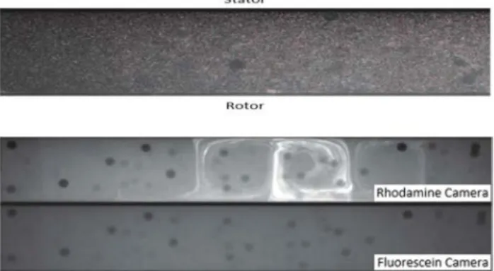
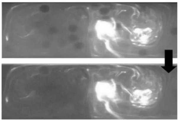
Fig. 4 Top: PIV image obtained in the presence of 1.5 mm beads, the image is cropped to fit with the region of interest and rotated by 90◦ .
Bottom: Two simultaneous acquisitions of the PLIF rhodamine WT image (top) and the fluorescein image (bottom). Case of a 4% volume concentration of 1.5 mm beads in TVF regime ( Re = 90)
velocity vector field in the cross section of the flow.
Acqui-sition devices are presented in Fig. 7 (left).
2.2.2 PLIF measurements
Planar laser-induced fluorescence (PLIF) visualizes the evolution of fluorescent tracer concentration as in Nemri
et al. (2014) for single-phase flows. The presence of beads
in the flow requires the use of two PLIF channels. Indeed, the tracer can not penetrate the beads hence leaving dark holes in the laser sheet. Because of the high intensity that results while injecting the fluorescent tracer, a simple inten-sity threshold is not sufficient to detect the boundaries of the
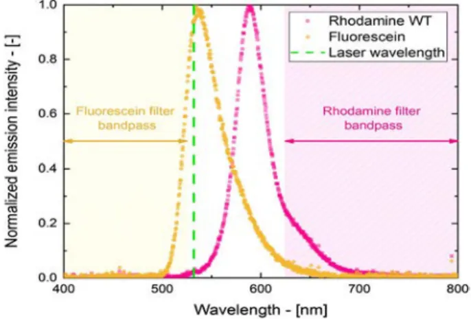
beads. Therefore, two fluorescent tracers are used (Fig. 4,
bottom). Fluorescein tracer in uniform concentration is used as a reference to easily detect the beads. Thanks to proper post-processing, dynamic masks with black holes are created at the bead locations. Rhodamine WT tracer is used to moni-tor the dye concentration during mixing, while the dynamic mask is superposed on this PLIF channel’s image to remove the light signal at the exact particle locations. The different emission spectrum of each fluorescent tracer (as shown in
Fig. 5) allows the fluorescent signals to be separated when
using the appropriate colored filters.
Two sCMOS cameras with 105 mm Nikon lenses are used to separate the information of each fluorophore. A field sepa-rator is implemented that dispatch the same image to the two cameras. Two high-pass filters (at 625 nm) allow to recover a maximum rhodamine light intensity by cutting off part of the fluorescein and PIV particles emitted light. Addition-ally, two low-pass filters (at 525 nm) are mounted on the second camera to cut off all the emission signal from the rhodamine and PIV particles. Using two identical filters on each camera improves the separation quality by increasing the optical density.
The PIV camera and the two PLIF cameras are sCMOS cameras with sensors of 2560 × 2160 pixels ( 6.5 μm × 6.5 μm
size). The calibration factors of respectively 0.017 mm/pixel and 0.034 mm/pixel have been measured using a calibration target placed in the investigation area. The visualization fields of the PLIF are larger than the one used for PIV ( 74 × 88 mm ), due to higher resolution required in PIV than in PLIF. Hence, a geometrical adjustment of the corresponding images between the fluorescein and the rhodamine image recording was
applied. The PLIF device is shown in Fig. 7 (right).
A 25 mg/L rhodamine concentration provides optimal opti-cal signal for our sCMOS (16 bits) camera. Based on prelimi-nary tests, only 70% of the 200 mJ laser power was applied to prevent any photobleaching effect. The local concentration is determined using calibration tabulated data. Different solu-tions of known rhodamine concentration were homogeneously dispersed in the column and the corresponding grey levels were measured with the PLIF rhodamine camera within the range of linear response. The background signal (before injec-tion) was systematically subtracted from the raw rhodamine PLIF images for each experiment. The corresponding calibra-tion funccalibra-tion is then used to measure the concentracalibra-tion spatial distribution in the following experiments.
For each experimental condition, the following procedure was used. The column is filled with the mixture of DMSO-KSCN-water and beads matched in density and refraction index. A fixed concentration of fluorescein, typically 0.5 mg/L is added to detect the beads and create the masks. Then, a given quantity of rhodamine (25 mg/L) and fluorescein (0.5 mg/L) is injected (0.5 mL at a rate of 3 mL/min, and 3 mL at 12 mL/ min respectively for TVF and WVF flow regimes). Injection is operated under controlled conditions at the center of the
measuring area through a capillary (Nemri et al. 2014;
Dher-bécourt et al. 2016). These injection conditions were selected
to minimize the flow perturbation.
2.3 Mixing quantification
Following the definition proposed by Ottino (1989) and the
previous investigations of Dusting and Balabani (2009) and
Nemri et al. (2014), a segregation index (Eq. 2) is used to
quantify mixing efficiency. The mixing index is based on the
concentration standard deviation 𝜎2
C(t) and the maximum mean
concentration 𝜎2
0(t) = C(t)(1 − C(t)):
2.3.1 Intra‑vortex mixing
We focus on the index of intra-vortex mixing, Irz , which
cor-responds to mixing within a single vortex along the radial and vertical directions.
(2)
I(t) = 𝜎
2 C(t)
𝜎02 .
To calculate Irz , an average image Crz(t) of each vortex is
calculated for every rotational period Tc:
Then, the variance 𝜎2
Crz(t) is calculated for each average
image from the mean concentration Crz(t) with K the number
of periods:
S is the number of pixels in the image of the vortex.
In all cases, the temporal evolution of the segregation index is a decreasing function of time, variance tends to zero until a uniform concentration is reached. Three specific times are defined to measure mixing efficiency: t1∕2 , t90 and t99 that
correspond to the time at which I0∕2 , I0∕10 and I0∕100 are
reached respectively, I0 corresponding to the injection time
which is used as a reference (Fig. 6). The mixing characteristic
times are scaled with the mean shear rate (Eq. 5):
The initial rate of decay, Rd , is also used as a measure of
mixing efficiency: (3) Crz(t) = ∑K k=1Ck(t) K . (4) ⎧ ⎪ ⎨ ⎪ ⎩ Crz(t) = ∑ r ∑ zCrz(t)∕C0 S 𝜎2C rz(t) = ∑ r ∑ z � Crz(t)∕C0−Crz(t) �2 S (5) 𝛤 = 𝛺Ri e . (6) R d= − dI(t) dt ||||t=0 ⋅ 1 𝛾I0.
2.4 Quantification of mixing for two‑phase flows 2.4.1 Coupled PIV/PLIF measurements
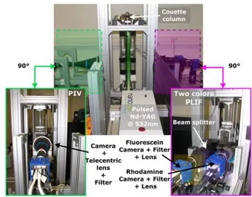
The experimental setup is illustrated in Fig. 7. All
equip-ments are assembled and synchronized together to perform PIV and PLIF sequence recording. Sub-steps of the post-processing procedure to access the mixing characteristics are
summarized in Fig. 8. PIV measurements provide the
veloc-ity fields which are used to characterize the vortices: minima of flow velocity stand at the vortex boundaries, which cor-respond to stagnation points. Using a uniform concentration of fluorescein, images are processed to extract the beads shapes, and build the corresponding dynamic masks which are then subtracted from the rhodamine images of the second PLIF channel. Finally, the corrected PLIF rhodamine images provide information on the concentration fields in each vor-tex to calculate the segregation indexes.
Fig. 6 Example of mixing time and initial rate of decay of Irz (open
symbols stand for raw data and dark symbols for the processed data using a smooth interpolating function with a sliding average filter) (Nemri et al. 2014)
Fig. 7 Experimental devices for the coupled PIV/PLIF measurements
The PIV results are used to extract the boundaries of the cellular vortices. To reduce noisy detection of the stagnation points in the velocity field, a large interrogation window with an important overlap has been chosen. Due to a longer light pathway at the rotor compared to the stator, a thinner interrogation window would result in strong fluctuations in the velocity field measurements.
The inter-correlation algorithm is initialized with
128× 128 cell size and decreased to 64 × 64 pixels with an
overlap percentage of 95%. This results in velocity fields composed of 855 × 337 vectors in the 2048 × 350 pixels image. The accuracy on the detection of stagnation points is typically less than 3 pixels.
Automatic thresholding and circular Hough detection
method (Kittler and Illingworth 1988) were used to
cre-ate the masks corresponding to the presence of beads in fluorescein images. Beads standing in front or behind the laser sheet are not detected, but they reduce light intensity in the images. The effect of these beads could be corrected by normalizing of rhodamine images by the fluorescein
images, as depicted in Fig. 9. The normalization procedure
consists in dividing, pixel by pixel, the light intensity of rhodamine images (minus background) by the light inten-sity of fluorescein images (registered on a field of view that matches perfectly the rhodamine images) corrected by the quantity of rhodamine PLIF signal that could pass through the low-pass 525 nm filter. A median filter (size 3 × 3 pixels) was applied on fluorescein images before normalization to reduce the weak spatial noise of the camera sensor.
2.5 Validation tests and reproducibility 2.5.1 Influence of dynamic masks
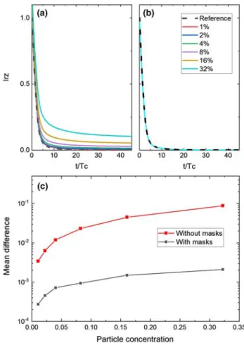
To estimate the impact of the dynamic masks on mixing characterization for high particle concentration, a specific analysis has been carried out. Based on a reference single-phase case, a synthetic image is generated, in which virtual
particles are randomly seeded. To this end, masks composed of dark disks were generated for concentrations ranging from
1 to 32% with 800 μm diameter (Fig. 10). The numerical
pro-cedure is implemented as follows. First, a region of interest corresponding to one vortex is extracted from the image and multiplied by random binarized masks (i.e., forcing 0 inside the beads mask and 1 outside). Then, the intra-vortex mixing
index Irz is calculated in two different ways: (1) excluding
the zeros from the calculation (which simulate the use of the dynamic masks), (2) considering all pixels in the image (naive post-processing ignoring the two-phase nature of the flow).
The whole process has been applied to more than 4000 frames to measure the difference between the two methods of calculating the segregation index. The mean difference between the two curves after normalization has been chosen as a dimensionless merit function for the robustness test, notably for its similarity with mixing index. A significant discrepancy exists for the naive post-processing which
considers the entire image (Fig. 11a), while in Fig. 11b, all
curves obtained with the mask correction collapsed onto the reference single-phase flow evolution. This test clearly shows that considering the correction provided by the dynamic masks reduces significantly the mean difference
(see Fig. 11c) on mixing quantification especially when the
particle volume concentration exceeds few percents. This study on synthetic images confirms the relevance of using two simultaneous PLIF images (one for mixing quantifica-tion and one for bead detecquantifica-tion/dynamic masks creaquantifica-tion). This reduces by more than one order of magnitude the error on quantification of mixing.
2.5.2 Robustness and reproducibility of experimental results
Additionally, three tests have been carried out to assess the robustness of the segregation indexes calculation. The con-clusion is drawn from 4% volume concentration experiments with 1.5 mm diameter beads.
Fig. 9 Top: Rhodamine image before normalization. Bottom:
• First the influence of borders detection is addressed. To this end, the borders of the region of interest were var-ied, i.e., by adding or removing 10 pixels on each border side (20 pixels on each vortex). A typical vortex has a length larger than 400 pixels and a width of 380 pixels.
As illustrated in Fig. 12 (top left), adding or removing
5% of the image does not change drastically the mixing quantification. The mean difference on mixing index is respectively 0.0043 and 0.00425 for each case, proving the accuracy of the vortex detection method.
• Second, the threshold used in the Hough algorithm for
the beads detection was varied by ±20% . The
refer-ence case in Fig. 12 (top right) is compared to the two
cases for which bead detection is respectively over or underestimated. The mean difference on mixing index is respectively 0.0026 and 0.0029 for each case. Again, no significant variation is observed.
• Third, the impact of applying a normalization process
to the image was evaluated. The normalization was applied either before or after the beads detection. A
small difference can be observed in Fig. 12 (bottom left),
but the mean difference on mixing index remains less
than 0.0106. Hence, normalization will not be considered in the following.
Finally, the reproducibility was assessed. In this aim, the same experiment has been repeated twice (4% volume
con-centration of 0.8 mm diameter beads). As shown in Fig. 12
(bottom right), the Irz curves measured in the two cases are
very close, the mean difference on mixing quantification is 0.0073 demonstrating the robustness of the processing.
3 Measurements of mixing in two‑phase
flows
Applying the procedure detailed in previous sections, the effect of the dispersed phase on the intra-vortex mixing has
been studied using the segregation index evolution Irz(t)
and the corresponding mixing times. Mixing is quantified
by both the initial rate of decay, Rd , of the segregation index,
and the time required to obtain full mixing t90 . Time scales
are made dimensionless using the mean shear rate. While Rd
measures mixing efficiency in the first instants after tracer
dye injection, t90 rather gives an estimate of the time required
for complete mixing of the tracer.
Three particle sizes have been selected: 0.8 mm, 1 mm and 1.5 mm diameter. Although particles are neutrally buoy-ant, they are not following the fluid streamlines. Indeed, finite size effects coupled to the mean shear and secondary flows are likely to yield hydrodynamic interactions, particle collisions and, therefore, trajectory fluctuations. The size ratio between the particle diameter and the gap between cyl-inders ranges from 0.073 to 0.14. The size of the vortices is typically similar to the gap width when the axial wave-length is 𝜆 = 2e . Particle volume concentration is varied from 0% (single-phase flow) to 8% , which corresponds to
Fig. 11 a Irz as a function of time without dynamic masks correction,
b Irz as a function of time with dynamic masks correction, c evolution
of relative error with increasing volume fraction of particles
0 10 20 30 40 50 t/Tc 0 0 2 0 4 0 6 0 8 1 Irz with mask 20 Pixels +20 Pixels 0 10 20 30 40 50 t/Tc 0 0 2 0 4 0 6 0 8 1 Irz calculated threshold threshold 20% threshold +20% 0 10 20 30 40 50 t/Tc 0 0 2 0 4 0 6 0 8 1 Irz without normalization with normalization 0 100 200 300 400 500 t/Tc 0 0 2 0 4 0 6 0 8 1 Irz Experiment1 Experiment2
Fig. 12 Sensitivity analysis on Irz : (top left) adding or removing
20 pixels, (top right) varying the threshold, (bottom left) with and without normalization and (bottom right) repeating the same experi-ment twice
dilute or moderately concentrated suspensions. Non-linear effects due to multibody hydrodynamic interactions is antici-pated to play a role in mixing enhancement. Two different hydrodynamic regimes are investigated, Taylor Vortex Flow (TVF) and Wavy Vortex Flow (WVF). The results section is organized as follows: effect of particulate concentration is investigated first, then the effect of particle size is addressed. Mixing in the radial direction is very fast, and we consider only the intra-vortex mixing in a vertical plane correspond-ing to Irz.
3.1 Effect of the particle concentration
We study the influence of the particle concentration while fixing the particle size for the two different flow patterns. To properly measure mixing enhancement, we have cho-sen flow patterns with a fixed wavelength at a prescribed Reynolds number. This is operated by selecting carefully the experimental procedure to have reproducible hydrodynamic properties. The rotor achieves its final rotation rate with a controlled ramp of acceleration.
3.1.1 TVF regime (Re = 100)
In the TVF regime, the single-phase flow is steady. There-fore, the presence of particles is the only source of veloc-ity fluctuations that couple to stretching and folding of dye streaklines close to stagnation points between vortices. Shear-induced particle agitation due to the radial gradient of azimuthal velocity participates to mixing by the carry-ing fluid flow. The results for particle diameters 1 mm and
1.5 mm are shown in Figs. 13 and 14, varying the
parti-cle concentration from 2 to 8%. We observe an increase of
the initial rate of temporal decrease of Irz in the two-phase
configurations, and a reduction of the time required for full mixing, as well. Clearly, the collective effect of particles enhances mixing when concentration increases for a given flow configuration. As shown in figures and tables, while the enhancement of mixing is very similar during the early stages after tracer injection, larger particles yield signifi-cant reduction of the time required to achieve homogeneous
spatial distribution of dye (corresponding to Irz= 0 ). The
mixing time is reduced by a factor 3 at 2% and almost a fac-tor 5 at 4% for 1 mm particles. Big particles are dragging more dyed fluid due to an increase of the flow perturbation by finite size effect. The results do not show a linear scaling with concentration as expected in a very dilute regime.
3.1.2 WVF regime (Re = 600)
At higher Reynolds numbers, the flow exhibits unsteady secondary flows which are reinforced by the shear-induced agitation of particles. In the single-phase flow, azimuthal
100 200 300 400 500 600 700 800 900 1000 t 0 0.1 0.2 0.3 0.4 0.5 0.6 0.7 0.8 0.9 1 Irz single-phase 2% 1 mm 4% 1 mm Concentration γt1/2 γt90 Rd Single-phase 101 930 0.0068 2% 54 314 0.0107 4% 42 188 0.0156
Fig. 13 Influence of the particle concentration on the intra-vortex mixing Irz in TVF regime for particle size of 1 mm
(Re = 100, 𝜆 = 2.25e ). Mixing times and initial decay rates are reported in the table
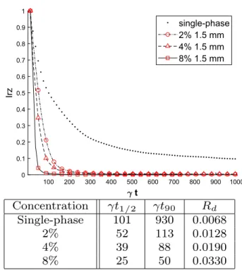
100 200 300 400 500 600 700 800 900 1000 t 0 0.1 0.2 0.3 0.4 0.5 0.6 0.7 0.8 0.9 1 Irz single-phase 2% 1.5 mm 4% 1.5 mm 8% 1.5 mm Concentration γt1/2 γt90 Rd Single-phase 101 930 0.0068 2% 52 113 0.0128 4% 39 88 0.0190 8% 25 50 0.0330
Fig. 14 Influence of the particle concentration on the intra-vortex mixing Irz in TVF regime for particle size of 1.5 mm
(Re = 100, 𝜆 = 2.25e ). Mixing times and initial decay rates are reported in the table
oscillations of the vortices participate to enhanced mixing compared to the steady TVF flow patterns. Similar con-clusions can be drawn in the WVF regime. According to
Figs. 15 and 16, increasing the suspension concentration
from 1 to 4% promotes intra-vortex mixing. Both indicators (increase of initial rate of decay and reduction of total time to reach complete mixing) evolve with the concentration evidencing the role of particles in enhanced mixing due to collective effects. Larger particle size has also a favorable
effect on mixing. The mixing time t90 is typically reduced by
a factor 3 when the concentration reaches 4%.
3.2 Effect of the particle size
To investigate the influence of the particle size, the particle diameter was changed under fixed flow conditions (particle volume concentration and flow regime).
3.2.1 TVF regime
As shown in Fig. 17, for a particle concentration equal to
1%, Irz decreases faster when the particle size increases from
0.8 to 1.5 mm. Time needed to reach a uniform distribution of the tracer is lower for the 1.5 mm beads than for 0.8 mm. So mixing for larger beads is faster and more efficient than
for small ones in the TVF regime. As reported in Fig. 17,
larger particle size leads to stronger initial decay rate: Rd
is multiplied by a factor 6 compared to single-phase flow configuration. Moreover, it can be observed that mixing enhancement varies with the square of particle size which
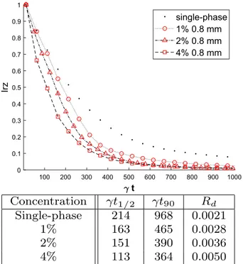
100 200 300 400 500 600 700 800 900 1000 t 0 0.1 0.2 0.3 0.4 0.5 0.6 0.7 0.8 0.9 1 Irz single-phase 1% 0.8 mm 2% 0.8 mm 4% 0.8 mm Concentration γt1/2 γt90 Rd Single-phase 214 968 0.0021 1% 163 465 0.0028 2% 151 390 0.0036 4% 113 364 0.0050
Fig. 15 Influence of the particle concentration on the intra-vortex mixing Irz in WVF regime for particle size of 0.8 mm
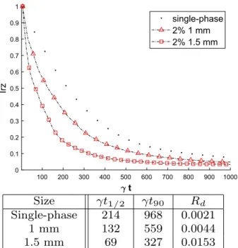
(Re = 600, 𝜆 = 2e ). Mixing times and initial decay rates are reported in the table 100 200 300 400 500 600 700 800 900 1000 t 0 0.1 0.2 0.3 0.4 0.5 0.6 0.7 0.8 0.9 1 Irz single-phase 2% 1 mm 4% 1 mm Concentration γt1/2 γt90 Rd Single-phase 214 968 0.0021 2% 132 559 0.0044 4% 88 289 0.0069
Fig. 16 Influence of the particle concentration on the intra-vortex mixing Irz in WVF regime for particle size of 1 mm
(Re = 600, 𝜆 = 2e ). Mixing times and initial decay rates are reported in the table 100 200 300 400 500 600 700 800 900 1000 t 0 0.1 0.2 0.3 0.4 0.5 0.6 0.7 0.8 0.9 1 Irz single-phase 1% 0.8 mm 1% 1 mm 1% 1.5 mm Size γt1/2 γt90 Rd Single-phase 264 1521 0.0023 0.8 mm 163 515 0.0029 1 mm 63 327 0.0111 1.5 mm 50 138 0.0140
Fig. 17 Influence of the particle size on the intra-vortex mixing Irz
in TVF regime ( Re = 100 , 𝜆 = 2e ) for particle concentration of 1%. Mixing times and initial decay rates are reported in the table
can be related to the surface in contact with the dyed liq-uid. Dye in the vicinity of the particle surface is dragged along the particle pathways and participates to mixing across streamlines.
3.2.2 WVF regime
Similar conclusions can be drawn in WVF, as illustrated in
Fig. 18. Intra-vortex mixing with larger beads is more
effi-cient in the WVF regime due to enhancement of fluid flow fluctuations by the particle agitation. In this dilute regime (concentration equal to 2%), getting homogeneous tracer distribution is typically 3 times faster than for single-phase
WVF configuration, while the initial rate of Irz decay is also
significantly increased (see Fig. 18).
4 Conclusion
We have carried out an experimental characterization of tracer mixing in the Taylor–Couette flow configuration. More specifically, we have measured the enhancement of mixing efficiency by solid particles with various sizes and volume concentrations. Particles are neutrally buoy-ant and the ratio between the particle diameter and the gap width between cylinders ranges from 0.073 to 0.14. A spe-cific attention has been paid to the Planar Laser-Induced Fluorescence (PLIF) measurements due to the presence of particles. Both density and refractive indexes of particles
were matched to fluid properties. The presence of beads in the flow requires to use two PLIF channels and the unsteady deformation of the vortices for WVF is measured by PIV (allowing detection of the vortex boundaries for the determi-nation of intra-vortex mixing). Systematic analysis and error quantification of the successive steps of image processing have been thoroughly discussed. We have shown that the determination of mixing times is robust over the range of investigated physical parameters.
With this method, the effect of dilute (1–2%) and moder-ately concentrated (4–8%) suspensions is compared through mixing indicators in the Taylor Vortex Flow and Wavy Vor-tex Flow regimes. The conclusion drawn from the exper-imental results is a clear and systematic enhancement of mixing under two-phase flow conditions. Both the particle size and concentration promote mixing i) during the early stages following dye injection, ii) on the long time behav-iour towards homogeneous spatial distribution of tracer. Due to the finite size of particles interacting with the flow, yielding shear-induced hydrodynamic interactions and col-lisions, mixing is significantly enhanced in dilute suspen-sions compared to the single-phase flow. The effect is further enhanced by large particles. While particles are crossing the fluid streamlines, they drag fluid and participate to stretching and folding of tracer concentration spatial gradients. This mechanism scales with the square of the particle radius, because the dye in the boundary layer of the particle sur-face is transported along particle trajectories. These observa-tions regarding mixing in two-phase Taylor–Couette flows are consistent with the microscale mechanisms evidenced
by Souzy et al. (2017). The presence of particles has also
an effect on inter-vortex mixing. Some preliminary results
are available in Dherbécourt et al. (2016). PLIF
visualiza-tions have shown that particles standing close to stagnation points or lying between Taylor vortices enhance dye migra-tion from one vortex to its neighbors. Dye is conveyed by particles through closed streamlines between adjacent vorti-ces and enhance tracer axial dispersion. This is particularly effective for big particles.
Acknowledgements The authors would like to thank CEA for financial
support and the technical support of Moise Marchal (IMFT) and Hervé Roussel (CEA).
References
Andereck D, Liu SS, Swinney HL (1985) Flow regimes in a circular Couette system with independently rotating cylinders. J Fluid Mech 164:155–183
Bouche E, Cazin S, Roig V, Risso F (2013) Mixing in a swarm of bub-bles rising in a confined cell measured by mean of PLIF with two different dyes. Exp Fluids 54(6):1552
Bruchhausen M, Guillard F, Lemoine F (2005) Instantaneous measure-ment of two-dimensional temperature distributions by means of
100 200 300 400 500 600 700 800 900 1000 t 0 0.1 0.2 0.3 0.4 0.5 0.6 0.7 0.8 0.9 1 Irz single-phase 2% 1 mm 2% 1.5 mm Size γt1/2 γt90 Rd Single-phase 214 968 0.0021 1 mm 132 559 0.0044 1.5 mm 69 327 0.0153
Fig. 18 Influence of the particle size on the intra-vortex mixing Irz
in WVF regime ( Re = 600 , 𝜆 = 2e ) for particle concentration of 2%. Mixing times and initial decay rates are reported in the table
two-color planar laser induced fluorescence (PLIF). Exp Fluids 38(1):123–131
Campero RJ, Vigil RD (1997) Axial dispersion during low Reynolds number Taylor–Couette flow: intra vortex mixing effect. Chem Eng J 52:3305–3310
Coles D (1965) Transitions in circular Couette flow. J Fluid Mech 21:385–425
Davis MW, Weber EJ (1960) Liquid–liquid extraction between rotating concentric cylinders. Ind Eng Chem 52:929–934
Desmet G, Verelst H, Baron GV (1996a) Local and global dispersion effect in Couette–Taylor flow—I. Description and modeling of the dispersion effects. Chem Eng J 51:1287–1298
Desmet G, Verelst H, Baron GV (1996b) Local and global disper-sion effect in Couette–Taylor flow—II. Quantitative measure-ments and discussion of the reactor performance. Chem Eng J 51(8):1299–1309
Dherbécourt D, Charton S, Lamadie F, Cazin S, Climent E (2016) Experimental study of enhanced mixing induced by particles in Taylor–Couette flows. Chem Eng Res Des 108:109–117 Dussol D, Druault P, Mallat B, Delacroix S, Germain G (2016)
Auto-matic dynamic mask extraction for PIV images containing an unsteady interface, bubbles, and a moving structure. Comptes Rendus Mécanique 344:464–478
Dusting J, Balabani S (2009) Mixing in Taylor–Couette reactor in the non wavy flow regime. Chem Eng Sci 64:3103–3111
Dutcher C, Muller SJ (2009) Spatio-temporal mode dynamics and higher order transitions in high aspect ratio newtonian Taylor– Couette flows. J Fluid Mech 641:85–113
Esser A, Grossmann R (1996) Analytic expression for Taylor–Couette stability boundary. Phys Fluids 8:1814–1819
Kataoka K, Takigawa T (1981) Intermixing over cell boundary between Taylor vortices. AIChE J 27:504–508
Kataoka K, Hongo T, Fugatawa M (1975) Ideal plug-flow properties of Taylor-vortex flow. J Chem Eng Jpn 8:472–476
Kataoka K, Doi H, Komai T (1977) Heat and mass transfer in Taylor-vortex flow with constant axial flow rate. Int J Heat Mass Transf 57:472–476
Kittler J, Illingworth J (1988) A survey of the hough transform. Com-put Vis Graph Image Process 44:87–116
Lanoë JY (2002) Performances d’une colonne d’extraction liquide-liquide miniature basée sur un écoulement de Taylor–Couette. In: ATALANTE conference, Scientific report, CEA, pp 244–251 Lindken R, Merzkirch W (2002) A novel PIV technique for measure-ments in multiphase flows and its application to two-phase bubbly flows. Exp Fluids 33(6):814–825
Majji S, Banerjee M, Morris J (2018) Inertial flow transitions of a sus-pension in Taylor–Couette geometry. J Fluid Mech 835:936–969 Metzger B, Rahli O, Yin X (2013) Heat transfer across sheared sus-pensions: role of the shear-induced diffusion. J Fluid Mech 724:527–552
Nemri M, Climent E, Charton S, Lanoe JY, Ode D (2013) Experimen-tal and numerical investigation on mixing and axial dispersion in Taylor–Couette flow patterns. Chem Eng Res Des 91:2346–2354 Nemri M, Cazin S, Charton S, Climent E (2014) Experimental inves-tigation of mixing and axial dispersion in Taylor–Couette flow patterns. Exp Fluids 55:1769
Nemri M, Charton S, Climent E (2016) Mixing and axial dispersion in Taylor–Couette flows: the effect of the flow regime. Chem Eng Sci 139:109–124
Ottino JM (1989) The kinematics of mixing: stretching, chaos and transport. The Press Syndicate of the University of Cambridge, Cambridge
Rudman M (1998) Mixing and particle dispersion in the wavy vortex regime of Taylor–Couette flow. AIChE J 44(5):1015–1026 Souzy M, Lhuissier H, Villermaux E, Metzger B (2017) Stretching
and mixing in sheared particulate suspensions. J Fluid Mech 812:611–635
Tam WY, Swinney HL (1987) Mass transport in turbulent Taylor–Cou-ette flow. Phys Rev A 36:1374–1381
Wilkinson N, Dutcher C (2018) Axial mixing and vortex stability to in situ radial injection in Taylor–Couette laminar and turbulent flows. J Fluid Mech 854:324–347