Generalization of Catalan combinatorics to the context of graphs

(1)

- - -

-UNIVERSITÉ DU QUÉBEC À MONTRÉAL

GENERALIZATION OF CATALAN COMBINATORICS TO THE CONTEXT OF

GRAPHS

THE SIS

PRESENTED

IN PARTIAL FULFILLMENT

OF THE MASTER'

S DEGREE IN MATHEMATICS

BY

MARJAN RASHTCHI

(2)

UNIVERSITÉ DU QUÉBEC À MONTRÉAL

Service des bibliothèques

Avertissement

La diffusion de ce mémoire se fait dans le respect des droits de son auteur, qui a signé

le formulaire Autorisation de reproduire et de diffuser un travail de recherche de cycles

supérieurs (SDU

-522

-

Rév.07 -2011). Cette autorisation stipule que

«conformément à

l'article 11 du Règlement no 8 des études de cycles supérieurs

, [l

'auteur] concède

à

l'Université du Québec

à

Montréal une licence non exclusive d'utilisation et de

publication de la totalité ou d'une partie importante de [son] travail de recherche pour

des fins pédagogiques et non commerciales

.

Plus précisément,

[l

'

auteur] autorise

l

'

Université du Québec à

Montréal

à

reproduire

,

diffuser, prêter

,

distribuer ou vendre des

copies de [son] travail de recherche

à

des fins non commerciales sur quelque support

que ce soit, y compris l'Internet. Cette licence et cette autorisation n

'

entraînent pas une

renonciation de [la] part [de l

'

auteur]

à

[ses] droits moraux ni

à

[ses] droits de propriété

intellectuelle.

Sauf entente contraire,

[l

'auteur] conserve la liberté de diffuser et de

commercialiser ou non ce travail dont [il] possède un exemplaire

.»

(3)

UNIVERSITÉ DU QUÉBEC À MONTRÉAL

GÉNÉRALISATION DE LA COMBINATOIRE DE CATALAN AU CONTEXTE

DES GRAPHES

MÉMOIRE

PRÉSENTÉE

COMME EXIGENCE PARTIELLE

DE LA MAÎTRISE EN MATHÉMATIQUES

PAR

MARJAN RASHTCHI

(4)

(5)

ACKNOWLEDGEMENT

Firstly, I would like to express my sincere gratitude to my supervisor, Prof. François Bergeron for the continuons support of my Master study and related research, for his patience, motivation, and immense knowledge. His guidance helped me in ail the time of research and writing of this thesis. I could not have imagined having a better advisor and mentor for my Master study.

I am also very grateful to my program's director Dr. Olivier Collin who helped me a lot through my study.

I must acknowledge as weil ali the professors and friends at LaCIM who in pired and supported me and my efforts over these years. Particularly, I need to expre s my gratitude and deep appreciation to Jose Eduardo Blazek, Alejandro Morales, Amy Pang, and Yannic Vargas Lozada.

Last but not the !east, I would like to thank my parents who not only tolerated my absence, but also supported me while I was away fTom home, and to my brother for upporting me tJu·oughout writing this thesis. Also, I would like to especially thank my hu band, who is al ways there cheering me up and stands by me th.rough the good times and bad.

(6)

(7)

LIST OF TABLES LIST OF FIGURES RÉSUMÉ . . ABSTRACT INTRODUCTION CHAPTER I

40

41 45 45 48 48 50 52 53 53 54 55 55 56 57 59

(9)

- - - -- - - ---

-LIST OF TABLES

Tableau Page

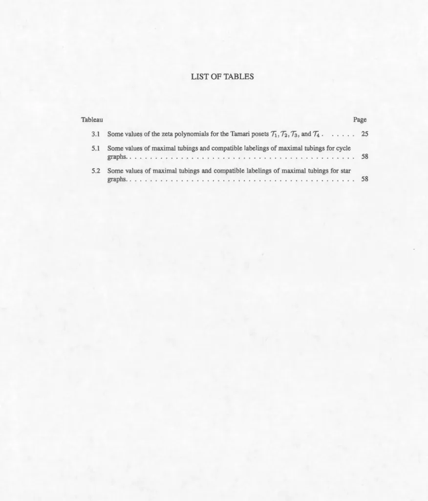
3.1 Sorne values of the zeta polynorrlials for the Tamari posets Ti

,

0. ,

T3

,

and

T4

.

25 5.1 Sorne values of maximal tubings and compatible labelings of maximal tubings for cycle

graphs. . . . . . . . . . . . . . . . . . . . . . . . . . . . . 58 5.2 Sorne values of maximal tubings and compatible labelings of maximal tubings for star

(10)

(11)

LIST OF FIGURES

Figure

1.1 A graph.

1.2 Illustration of a subgraph (left) and an induced subgraph (right) of a graph .. 1.3 A graph with three connected components.

1.4 The poset of subsets of {1, 2, 3} under inclusion. 1.5 A path, complete, and cycle graphs in terms of poset. 1.6 Poset P .

.

. . . . .

1.7 Weak order on §3 . .

2.1 The set B3, of binary trees with 3 nodes.

2.2 The set C3 , of complete binary trees with 7 nodes .. 2.3 The set D3, of Dyck paths of size 3.

2.4 A Dyck path with composition 21 ..

2.5 Non-Dyck path (in red), and its reflected part (in black) . 2.6 The post-order of this tree ise, j, g, d, h, c, b, i, a . .. 2.7 Transforming the complete binary tree to Dyck path.

Page 3 4 5 6 6 8 11 13 14 14 15 15 17 17 2.8 Dyck path which meets the diagonal (left one), and does not meet the diagonal (right one). 18 2.9 Transforming the Dyck path

SESE to a complete binary

tree. . . . . . . 18 2.10 General forrn of transforming Dyck path

SM E to

a complete binary tree.

2.11 Transforming the Dyck path

SSESESEE to

a complete binary tree. 2.12 Sequence (1, 1, 1, 3) --+ Dyck path

SSSEESEE.

2.13

Dyck

path

SSEESESE---+

sequence(1,1,3,4). 3.1

3.2

3.3

3.4

The Tamari lattice

T3

.

The enumeration of intervals in Tamari lattice

T3

.

Right-rotation. . . .

Notion of t 1 ""* t2 . 19 19 20 20 24 24 25 26

(12)

xii

3.5 The Tamari lattice of complete binary trees for n

=

3 (left) and n

=

4 (right). 3.6 The Tamari latt.ice of binary trees for n

=

3 (left) and n

=

4 (right).

3.7 otion of d1 ~ d2 . . . · · · · · · · · · 3.8 The Tamari lanice of Dyck paths for n

= 3 (left) and n

= 4 (

right) .. 3.9 Two triangulations

T

and

T'

are being related by an edge f'lip. 4. J 211 is a parking function of length 3 .

4.2 Define function

f

on the set of labels.

4.3 Parking functions over one Dyck path of size 3 .

4.4 Enumeration of Dyck paths with _(r1

=

1, r2

=

1,

rs

= 0) .

4.5 How O" permutes the labels of a labeled Dyck path of D4.

4.6 Stable labeled Dyck paths of D3 by O". 4.7

4.8 Parking functions over a complete binary tree of C3

.

4.9 Parking functions over one complete binary tTee of size 3 .

4.10 The Tamari po set 0, with the associated bounded increasing sequences. 5.1 Val id tubings of sorne connected graphs ..

5.2 1nvalid tubings of sorne connected graphs.

5.3 Val id tubings of sorne graphs with severa! connected components. 5.4 Inval id tubings of sorne graphs with severa! connected components. 5.5 Poset of tubings of a path graph with 3 nodes.

5.6 Representation offunction

f.

26 27 27 28 29 32 34 35 36 37 37 38 40 41 42 46 46 46 46 47 48 5.7 Transforming a maximal tubing of a path graph to the corresponding binary tree. 49 5.8 Transforming a binary tree to the corresponding maximal tubing of a path graph. 50 5.9 Notion of

U1

~

U2.

. .

.

. .

. . . . .

.

. .

.

. . . .

. .

. . .

.

. .

.

. .

50 5.10 The Tamari lattice th at results from maximal tubings on the pa th graph for n=3 (left) and

n=4 (right). . . . . . . . . . . . . . . . . . 51 5.11 Pushing the tubes in order from smallest one, right to Jeft. . 51 5.12 A compatible labeling for a path graph with five vertices. . 52 5.13 Parking functions on the maximal tubing of a 3-path graph. 53

(13)

Xlii

5.14 A covering relation in the weak order on permutations. . . . . . . . . . . . . . . . 54 5.15 The Jattice that results from maximal tubings on the complete graph with 3 vertices. 54

5.16 The lattice that result from maximal tubings on the three disjoint nodes. 55

5.17 The lattice th at results from maximal tubings on the star graph S2 . 56

5.18 A compatible labeling for a cycle graph with three vertices. . . . . 56

(14)

(15)

RÉSUMÉ

Il est question dans le présent document de certaines familles d'objets mathématiques dont la cardinalité se dénombre par la célèbre suite des nombres de Catalan. Nous nous concentrons sur certaines propriétés

du treillis de Tamari. Nous considérons aussi les relations entre ces objets et les fonctions de statio n-nement. Afin d'étendre ces constructions à d'autres contextes, nous introduisons la notion de« tube de graphe >>. Pour les graphes de chemins, ceci retrouve la configuration de Catalan. Par cette analogie,

nous pouvons généraliser à d'autres familles de graphes tels que les graphes complets, cycliques, etc.

Mots-clés: Nombre de Catalan, objets de Catalan, treil lies de Tamari, polynôme de zeta, fonctions de stationnement, tube de graphe.

(16)

(17)

ABSTRACT

In the present document we investi gate families of mathematical objects counted by the fa mous sequence of Catalan numbers. We are interested in properties of sorne structures on uch families known as the Tamari lattices. We consider relations between those objects and parking functions. To extend such constructions to other contexts, we introduce the notion of "graph tubing". For pa th graphs, thi recovers the Catalan setup. Using this analogy, we can generalize the theory to other nice families of graphs such as complete graphs, cycle graphs, etc.

Keywords: Catalan numbers, Catalan objects, Tamar lattice, zeta polynomials, parking functions, graph tubing.

(18)

(19)

--- ---

-INTRODUCTION

Catalan numbers have always been considered as an important integer sequence in combinatorics with severa! characterization, and there are severa! interesting families of mathematical objects counted by these numbers, which are named Catalan objects. On the other hand, Dov Tamari in [15, 1962] in -troduced a lattice structure on the family of well-formed parentheses whose number of elements is the Catalan number. There are sorne interesting results on the Tamari lattice such as Chapoton's formula to count the number of intervals in this lattice. Furthermore, there are other combinatorial notions such as Parking functions, whose connections to Catalan objects are interesting. Any time a new farnily emerges whose elements are enumerated by the Catalan numbers, we are motivated to find the associated Tamari order on i ts po set.

In [5, 2005] M. Carr and S. Devadoss introduced the notion of "graph tubing" in which, specially for path graphs, the number of maximal tubings is the Catalan number. Hence maximal tubings of a path graph is y et another class of Catalan objects. In [Il, 2012] M. Roneo described a partial order on the set of tubings of a simple graph, which generalized the Tamari order on the set of tubings of path graphs. During the same year, S. Forcey in [8] generalized the Tamari order, and the weak order on permutations, to maximal tubing of a graph.

In the present work, our goal is to relate parking functions to maximal tubings of path graphs as a recent Catalan object. This opens the possibility of considering parking functions for maximal tubings of other "nice" families of graphs, such as complete graphs, cycle graphs, etc.

The first chapter of this monograph recalls sorne basic combinatorial notion namely: posets, intervals in posets, lattices, the zeta polynomial, Catalan numbers, and the symrnetric group §n· In the second chapter, we introduce sorne of the Catalan objects such as Dyck paths, Dyck words, binary trees, and complete binary trees. Although there are direct individual proof that the cardinality of Dyck paths, binary trees or other Catalan families are indeed given by Catalan numbers, we will rather prove this for just one case (Dyck paths), and then show that there are bijections linking other families to this specifie one. In Chapter 3, we translate the Tarnari lattice structure to the context of the considered families, and interpret the order direct! y in the relevant context. In Chapter 4, the properties of parking functions are discussed, and we consider how parking functions may be defined direct! y in each context. Also we ex-tend the enumeration of parking fun etions using zeta polynomials. We start Chapter 5 with the definition of tubing and its properties, and also we recall how to count the number of maximal tubings for sorne

(20)

2

special families of graphs, such as path graphs, complete graphs, and cycle graphs. We describe the Tamari order defined by Forcey, and continue with the spirit of parking functions in terms of maximal tubings of pa th graphs.

(21)

CHAPTERI

SOME BACKGROUND IN COMBINATORICS

In this chapter we introduce sorne combinatorial terminology such as graphs, posets, intervals in posets, lattices, zeta polynomials, Catalan numbers, and symmetric groups §n which will be used later .

1 .

1 Graph

s

A (simple) graph is a pair of sets, denoted G

=

(V,

E

), where

V is a fini te set and E is a subset of (~),

which stands for the set of pairs of elements in V. The set V is called the set of vertices (or nades), and

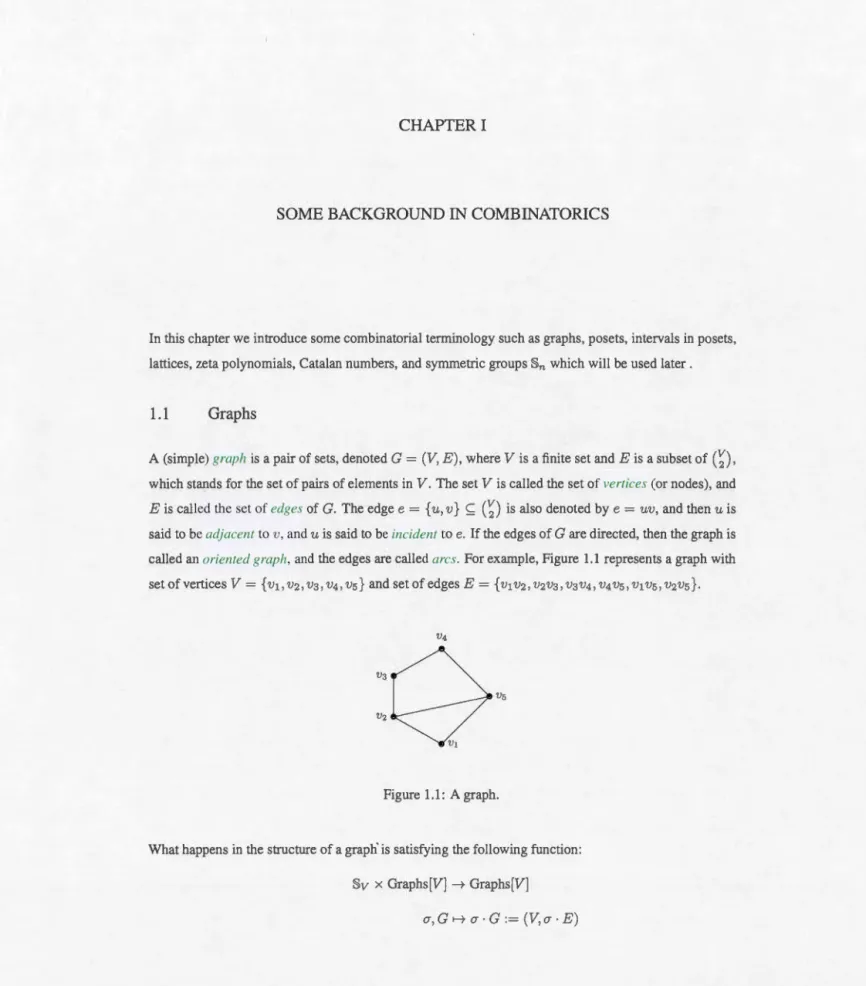
E is called the set of edges of G. The edge e = { u, v} ç:: (~) is also denoted by e = uv, and then u is said to be adjacent to v, and u is said to be incident to e. If the edges of Gare directed, then the graph is called an oriented graph, and the edges are called arcs. For example, Figure 1.1 represents a graph with set of vertices V = { v1, Vz, v3, V4, Vs} and set of edges E = { v1 vz, vzv3, V3V4, V4 vs, v1 Vs, vzvs}.

Vs

Figure 1.1: A graph.

What happens in the structure of a graph' is satisfying the following function: §v x Graphs(V] --+ Graphs(V]

(22)

- - - -- - - -- - --- -- - - --- - - -- - - - -- - -

-4

such that:

• §v :=

{a-

1 0': V -+ V}. (see Section 1.4) • Graphs(V] := {(V, E) 1 E Ç (~)}.

• O'·E:

=

{{O'

(

u

)

,O'

(v

)}

l

{u,

v

}

E

E}.

Then two graphs G₁and G₂are isomorphic if and only if there exists a function 0' in §v such that

O'

.

G

1 =

G

2 ,

denoted

G

1 "'

G

2 .

This is an equivalence relation. Hence a graph type (shape) is an equivalence clas for thi i omorphism relation

(G] E Graphs(V]/~·

We will informally refer to an equivalence class

(

G

]

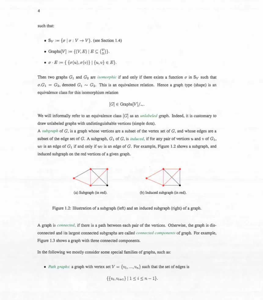
as an unlabeled graph. lndeed, it is customary to draw unlabeled graphs with undistinguishable vertices (simple dots).

A subgraph of G, i a graph whose vertices are a subset of the vertex set of G, and whose edges are a subset of the edge set of G. A subgraph, G 1 of G, is induced, if for any pair of vertices

u

and

v

of G 1,

uv

is an edge of G1 if and only if

uv

is an edge of G

.

For example, Figure 1.2 shows a subgraph, and induced subgraph on the red vertices of a given graph.

(a) Subgraph (in red). (b) !nduced subgraph (in red).

Figure 1.2: Illustration of a subgraph (left) and an induced ubgraph (right) of a graph.

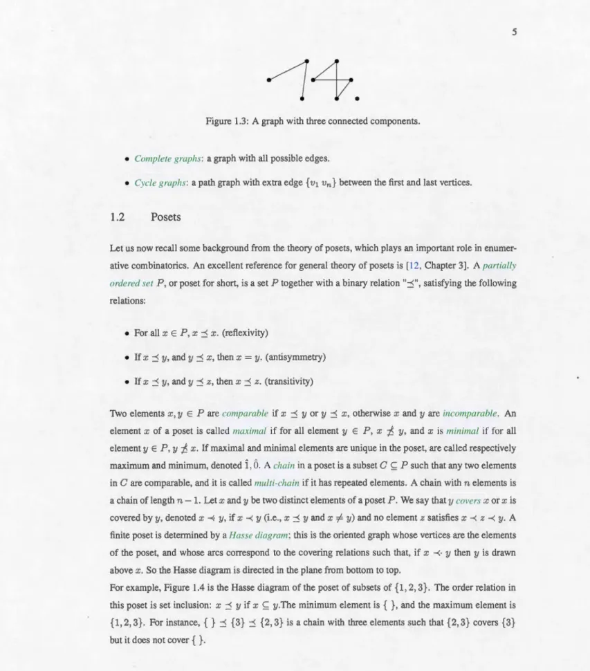
A graph is connected, if there is a path between each pair of the vertices. Otherwise, the graph is

dis-connected and its la.rgest connected subgraphs are cal led connected components of graph. For example, Figure 1.3 shows a graph with three connected components.

ln the following we mostly consider sorne special fa.milies of graphs, such as:

• Pa th graphs: a graph with vertex set V = { v1, ... ,

v

n} s

uch that the set of edges is

{{

v;

,vi+

d

I

l

:Si:::;

n- 1}.

(23)

5

~4

.

Figure 1.3: A graph with three connected components.

• Complete graphs: a graph with ail possible edges.

• Cycle graphs: a path graph with extra edge { v1 vn} between the first and last vertices.

1.2 Posets

Let us now recall sorne background from the theory of posets, which pla ys an important role in enum er-ative combinatorics. An excellent reference for general theory of posets is [12, Chapter 3]. A partially ordered set P, or poset for short, is a set P together with a binary relation ":j", satisfying the following relations:

• For ail x E

P

,

x :::5 x. (reflexivity)

• If x :::5 y, and y :::5 x, then x = y. (antisymrnetry)

• If x :::5 y, and y :::5 z, then x :::5 z. (transitivity)

Two elements x, y E Pare comparable if x :::5 y or y :::5 x, otherwise x and y are incomparable. An element x of a poset is called maximal if for ail element y E P, x

1:.

y, and x is minimal if for ail

element y E

P

,

y

1:.

x. If maximal and mjnimal elements are unique in the poset, are called respectively maximum and minimum, denoted

Î

,

Ô.

A chai11 in a poset is a subset C Ç P such that any two elements in C are comparable, and it is called mu/ti-chain if it has repeated elements. A chain with n elements is a chain of length n-1. Let x and y be two distinct elements of a poset P. We say that y covers x or x is covered by y, denoted x-<· y, if x-< y (i.e., x :::5 y and xi= y) and no element z satisfies x-< z -<y. A fini te poset is determined by a Hasse diagram; this is the oriented graph whose vertices are the elements of the poset, and whose arcs correspond to the covering relations such that, if x

-<·

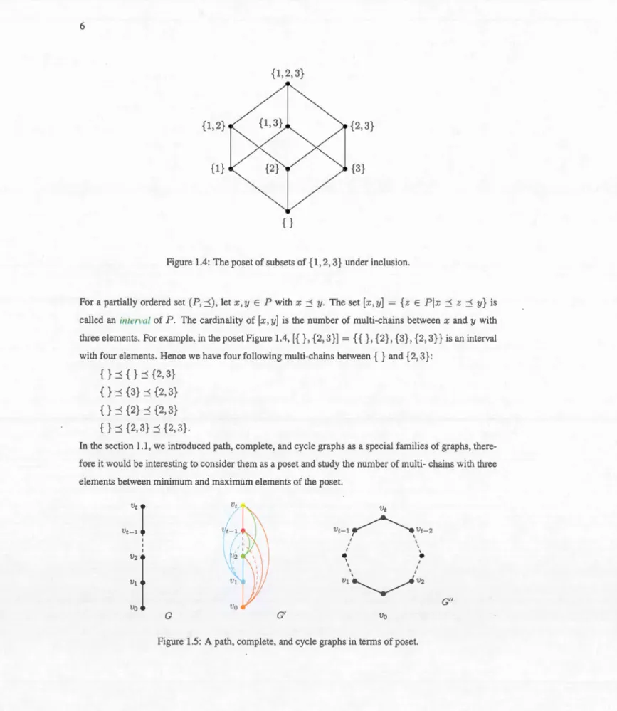
y then y is drawn above x. So the Hasse diagram is directed in the plane from bottom to top.

For example, Figure 1.4 is the Hasse diagram of the poset of subsets of {1, 2, 3}. The order relation in this poset is set inclusion: x :::5 y if x Ç y.The minimum element is { }, and the maximum element is {1, 2, 3}. For instance, { } :::5 {3} :::5 {2, 3} is a chain with three elements uch that {2, 3} covers {3} but itdoes notcover { }.

(24)

6

{1,2,3}

{1,2} {2,3}

{1}

{3}

{}

Figure 1.4: The po et of subsets of {1, 2, 3} under inclusion.

For a parti ally ordered set (P, ~), let x, y E P with x ~ y. The set [x, y]

=

{

z E

P

l

x ~ z ~

y}

is cal led an interval of P. The cardinality of [x, y] is the number of multi-chains between x and y with th.ree elements. For example, in the poset Figure 1.4, [ { } , {2, 3}]

=

{ {

}

,

{2}, {3}, {2, 3}} i an intervaJ with four elements. Hence we have four following multi-chains between {}and {2, 3}:

{} ~ {} ~ {2,3}

{ }

~

{3}

~

{2,

3}

{ }

~

{2}

~

{2, 3}

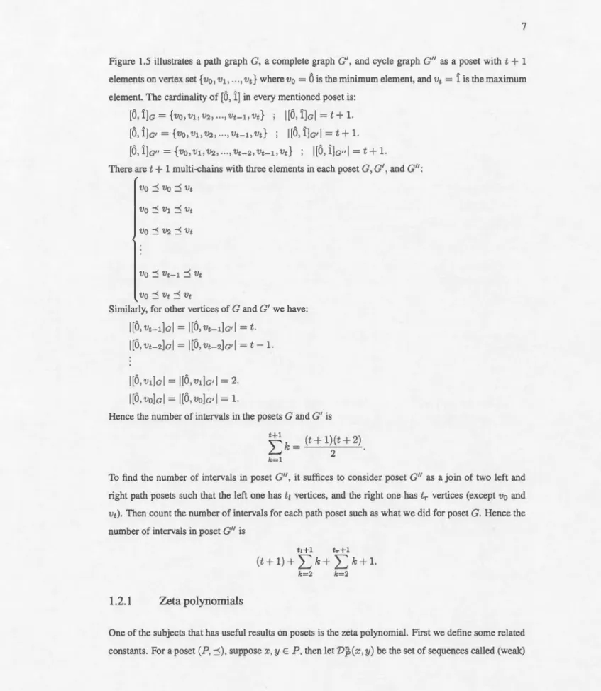
{} ~ {2,3} ~ {2,3}.

In the section 1.1, we introduced path, complete, and cycle graphs as a special familie of graphs, there-fore it w·oüld b interesting to consider them as a poset and study the nümber of mülti-chains with thrc;e elements between minimum and maximum elements of the poset.

Vt

I

Vt Vt-1

Vt

-

l

~

1 _\

Vt

-

2

1 1 1

• ~

f

~ 1 \ 1 \ 1 \ 1 VI V1~V2 G" va G Gl va

(25)

7

Figure 1.5 illustrates a path graph

G

,

a complete graph

G

',

and cycle graph

G"

as a poset with t + 1 elements on vertex set {

v

0 , v

1, ... ,

Vt

}

where

v

0

=

Ô

is the minimum element, and

Vt

= Î is the maximum element. The cardinality of

[

Ô

,

Î

]

in every mentioned poset is:

I[

Ô

, Î

]cl =

t

+

1.

[

Ô

,

Î

]c• =

{

vo,

v1,

v2

,

...

,

Vt-

1,

v

t}

I[

Ô

, Î]c•

1

=

t

+

1.

[

Ô

,

Î

]c"=

{

vo,v

1 ,v2,···,Vt-2,vt-1,vt};

I[Ô,

Î

]c"l=t+

l.

There aret+ 1 multi-chains with three elements in each poset

G

,

G

',

and G":

VQ

~

Vt-1

~

Vt

V

o

~

Vt

~

Vt

Similarly, for other vertices of G and G' we have:

I[

Ô

,vt-l

]c

l

= I[

Ô

,Vt-1]c•l

=

t

.

I

[Ô,

V

t

-

2 ]cl

= I[

Ô

,

V

t

-2]c•

1

=

t

-

1.

I

[Ô,v1Jcl

=

I[Ô

,

v1Jc•l =

2.

I[

Ô

,

v

o

]cl

=

I[

Ô

,

vo]c•l =

1.

Hence the number of intervals in the posets G and G' is

~

k

=

(t+ 1)(t+ 2)

L.J 2 .

k=1

To find the number of intervals in poset

G"

,

it suffices to consider poset

G"

as a join of two left and right path posets such that the left one has tt vertices, and the right one has

t,.

vertices (except v₀and

V

t).

Then count the number of intervals for each path poset such as what we did for poset G. Hence the number of intervals in poset G" is

t,+1 t,.+1

(t

+ 1) +

2:

k +

2:

k + 1.

k=2 k=2

1 .

2 .

1 Zet

a

polynomial

s

One of the subjects that has useful results on posets is the zeta polynomial. First we defi ne sorne related constants. For a poset (P, ~),suppose

x, y E

P, then let

'D

f>

(x

,

y) be the set of sequences called (weak)

(26)

8

chain defined as follows:

V

f,(x

,

y

)

:

=

{

(x

o

,

...

,Xn)

1

x= X

o

-<

X

1 -< .

.

. -<

Xn

=

y}

.

and let

C

?(x,

y

)

be the set of sequences called multi-chains defined as follows:

Cf,(x

,

y

)

:= {

(xo

, ... ,

xn)

1

x= xo

~ x1 ~ ... ~

Xn

=

y}.

The zera polynomial, Zp(n), for a poset P with minimal and maximal elements Ô,Î respectively, is defined as follows:

Zp(n) :=

IC

'J,(

Ô

,

Î)l.

As a polynomial inn, we have (see [12]):

Zp(n) =

L

(

~

)

I

V

~(

Ô

,

Î)l. k~O

(1 .2.1)

For example, for the poset P in Figure 1.6 with minimum element a and maximum element e, the zeta polynomial is:

Zp(n)

=

~

(

n

3

+

6n2- n). One gets the following binomial coefficient expansion:

This is so since: Zp(n)

=

(

7 )

l

{

(a

,e

)

}

l

+

G

)

l

{

(a

,

b

,e

)

,

(a

,

c

,e

)

,

(

a

,

d

,e

)}

l

+

(~)

l

{

(a

,

b

,c

,e

)

}

l.

c b e =

î

a

=

Ô

Figure 1.6: Poset

P .

d

As a result, we have

Zp(

2 )

= 5, oit means that the multi-chains with three elements count the elements

(27)

9

the poset.

We can a Iso calculate the zeta polynomial for posets of a pa th graph, a complete graph, and a cycle graph

of Figure 1.5 with n

+

1 vertices:

Za(n)

=

n

+ (t-

1 )

(~)

+

(t

-

2)

!

G)

+ (t-

3)

'(

:)

+ .. ·

This is so since:

Za(n)

=

(7)

l{(vo,vt)}l

+

G)

l

{

(vo,vl

,

vt), (vo,v2

,

Vt)

,

...

, (vo,Vt-l

,

vt)}l

+

G

)

l

{

(vo,vl,v2,vt)

,

(vo

,

vl

,

v3,vt),

...

, (vo,vl

,

Vt-l>Vt)

(vo

,

V2, V3

,

V

t

)

,

(vo

,

V2

,

V4

,

Vt)

,

· .

,

(vo

,

V2,

Vt-1

,

Vt)

(vo

,

Vt-2,

Vt-1, Vt

)}

l

+

".

TheZa' (n) is the same as the Za(n). For calculate Za" (n), G" as a jo in of two paths that the left one contains

t

1 vertices, and the right path contains

tr

vertices (except v0 and v1 ), we have the following polynomial:

za,(n)

=

n+(t-1)

(

~

)

+

(

tt-1

)

!

(

~

)

+(

tt-2

)

!

(

:)

+

· ·

· )

+

(

(t,.-

1 )

!

(

~

)

+(tr-

2 )!

(

:

)

+

·

· )

1 .

2 .2

Latti

c

e

s

An important class of posets is known as lanices. To introduce lanices, first recall sorne definitions. Let (P,

j)

be a partially ordered set. An upper bound of x, y E P is an element z E P satisfying x j z and y j z. A !east upper bound of x and y is an upper bound z such that every upper bound z' of x and y

satisfies z j z'. A !east upper bound of x and y is unique if it exists, and is called their join, denoted x V y. Similarly, a lower bound of x, y E P is an element z E P satisfying z j x and z j y. A greatest

lower bound of x and y is a lower bound z such that every lower bound z' of x and y satisfies z' j z. A greatest lower bound of x and y is unique if it exists, and is called their meet, denoted x 1\ y.

A lattice is a po et for which every pair of elements has a join and meet. A Jattice as an algebraic stmcture in terms of the operations

v

and /\, satisfies the following axioms:

• Commutative law: x V y =y V x, x 1\ y =y 1\ x.

• Associative law: x V (y V z) =(x

v

y) V z, x 1\ (y 1\ z) =(x 1\ y) 1\ z.

(28)

10

• Idempotent law: x V x = x 1\ x =x . • x 1\ y = x <=} :r;

v y

=y <=} x

::S

y.

For example, the poset in Figure 1.4 is a lattice that {1} V {3}

=

{1, 3}, and {1} 1\ {3}

=

{}

.

1.3 Catalan number

s

As illustrated by a famous exercise in Stanley's book [13], one of the best known integer sequences in

combinatorics is the sequence of Catalan numbers. Catala11 11umbers are defined by

C(n)

=

_1 (2n).

n+1 n (1.3.1)

In 1838, Belgian mathematician Eugëne Charles Catalan was the first to obtain what is now a standard formula for Catalan numbers. Small values of C(n) are:

1,1,2,5,14,42,132,429,1430, ...

The Catalan numbers satisfy the following recuiTence relation for n

>

0 where C(O)

=

1,

n

C(n +

1 )

=

L

C(k)C(n-k). (1.3.2)

k=O

As is frequently useful in combinatorics, we can try to calculate or geta formula for C(n) by using a generating function. This means that for a power series B(x) defined by

B(x) :=

L

C(n)xn,

n

in term of the generating function, we have

B(x)

=

1

+

xB(x)2,

which is simply a translation of the recursive definition of Catalan number (for more details see [3]). We will have many families of objects (grouped by "size"), such that the number of those objects in size

n is equal to C(n). For this reason, we will say that such objects are "Catalan objects". This will be the

subject of the next chapter.

1.4 Symmetric

g

roup

§n

The symmetric group

Sn

is the group of bijections of

[n] =

{

1 ,

...

,

n}

to itself. The cardinality of this set is equal to n!. A notation for the permutation that sends i --+ li is

(29)

11

A k-cyc/e permutation (or a cycle of length k) is a permutation that sends l; to li+1 for 1 ::::; i ::::; k - 1 and lk to 11, denoted

The same cycle can be written in severa! ways, by cyclically permuting the l_{1 .}For example, it a Iso can

be written as:

Two cycles (h l2 ... lk) and (l~ l~ ... l~,) are disjoint, when the sets {l1, ... ,lk} and {l1, ... ,l~,} are disjoint. Every permutation Œ E §n is expressible as a product of disjoint cycles unique! y, which is called

the cycle decomposition of CT. For example, Œ

=

25431 in §5 has a cycle decomposition (2 5 1)(3 4).

Let

U

~=l

n;

=

{1, 2, ... ,

n

}

be a partition of {1, 2, ... ,

n}

into k disjoint subsets. Th en the corresponding Young subgroup of §n, is the subgroup

where §n,

=

{CT

E §n : Œ(j)

=

j for ali j

fJ.

n;},

that consists of ln;l! of sucho-. This means that CT

permutes the elements of n;, and fixes the elements in the complement {1, 2, ... , n} \n;.

Fora permutation Œ in §n, an inversion setofŒ, denoted Inv(Œ), is thesetofpairs

(i,j)

withi

<

j

and

l;

>

l₁. For example, Inv(Œ = 312) =

{

(1, 2), (1, 3)}, because 11

=

3

>

l2

=

1 and

h

= 3 > l3

= 2.

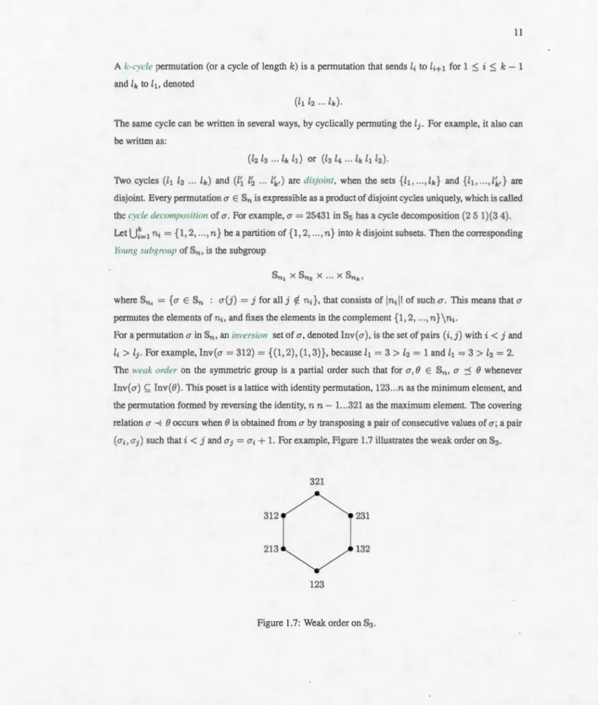
The weak arder on the symmetric group is a partial order such that for Œ, 8 E §n, CT

::S

8 whenever

lnv(Œ) Ç Inv(8). This poset is a lattice with identity permutation, 123 ... n as the minimum element, and the permutation formed by reversing the identity, n n-1...321 as the maximum element. The covering

relation CT

-<·

8 occurs when 8 is obtained from CT by transpo ing a pair of consecutive values of

Œ;

a pair

(Œ;, Œj) such that i

<

j and Œj = Œ;

+

1. For example, Figure 1.7 illustrates the weak order on §_{3 .}

321

312 231

213 132

123

(30)

(31)

CHAPTERII

SOME CATALAN OBJECTS

Stanley (see [13]) has compiled a list of more than 207 combinatorial abjects that are counted by the

Catalan numbers. Much of our story concem generalisations of the Catalan numbers and families of

mathematical abjects counted by these, which we call, Catalan objects. In this chapter we consider five families of Catalan abjects: binary trees, complete binary trees, Dyck paths, Dyck words, and bounded increasing sequences. We count the number of Dyck paths to see it is equal to the Catalan numbers, and

show that the other Catalan abjects bijective! y have the same cardinality.

2.1 Binary trees

Recall that a tree is an undirected, acyclic, connected graph. This means that any two nades are connected by exactly one simple path. A bùzary tree is an arrangement of nades and edges with root node on the

top, and by descending, every node is connected to at most two node , which are sa id to be its right and left children. The root node separates the binary tree into two right and left subtrees. Let us denote by

Bn

the set of ali binary trees with n nodes. The number of nodes of a binary tree i cal led the size of the

tree. The cardinality of

Bn

is equal to C(n). For example, Figure 2.1 shows the set of binary trees with three nodes.

(32)

14

2.2 Complete binary trees

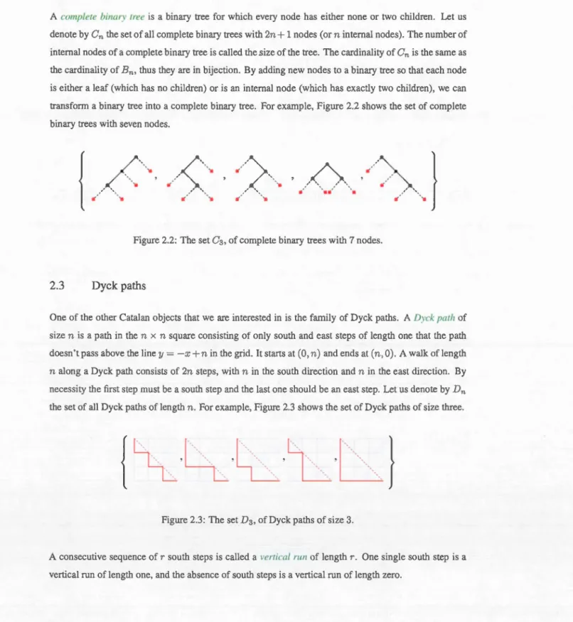
A complete binary tree is a binary tree for which every node has either none or two children. Let us

denote by Cn the set of ali complete binary trees with 2n+ 1 nodes (or n interna! nodes). The number of interna! nodes of a complete binary tree is ca lied the .size of the tree. The cardinality of Cn is the same as

the cardinality of

Bn,

thus they are in bijection. By adding new nodes to a binary tree so that each node is either a leaf (which has no child.ren) oris an interna! node (which has exact! y two children), we can transform a binary tree into a complete binary tree. For example, Figure 2.2 shows the set of complete

binary trees with seven nodes.

{

r/

.(.

·-.

· .

.

<

.:· ·

·

-.

,

·

.:

·>

· ·-.

.

'

.

...

<:>

.

..

.

...

.

,

· /

»

.

..

}

Figure 2.2: The set Ca, of complete binary trees with 7 nodes.

2.3 Dyck

paths

One of the other Catalan objects that we are interested in is the family of Dyck paths. A Dyck pa th of size n is a path in the n x n square consisting of only south and east steps of length one thal the path doesn't pass above the line y=

-x+

n in the grid. It start at (0,

n)

and ends at

(n,

0). A walk of length

n along a Dyck path consists of 2n steps, with n in the south direction and n in the east direction. By

neces iL y Lhe firsL slep mu L be a ouù1 Lep and the iast one should be an east tep. Let u denote by Dn

the set of all Dyck paths of length n. For example, Figure 2.3 shows the set of Dyck paths of size three.

Figure 2.3: The set

D

a

,

of Dyck paths of size 3.

A consecutive sequence of r south steps is called a vertical run of length r. One single south step is a vertical run of length one, and the absence of south steps is a vertical run of length zero.

(33)

15

For a Dyck path a E

D

n,

-y( a)

=

a1az ... an is called the composition of a if the i-th vertical run of a has length a; (for 1 ~ i ::::; n), and 2::~

1

a;

=

n. Clearly -y(a) is a composition of n. For example, Figure 2.4 illustrates a Dyck path in D3 with composition 21. ' ' ' _' ' Figure 2.4: A Dyck path with composition 21 .

2 .

3.

1 Count the

number

of Dy

c

k p

a

th

s

A random path in a square n x n, is a path with 2n steps (n south steps and n east steps, each of length one) that start at (0, n) and ends at (n, 0). Hence the total number of random paths with 2n steps is

A Dyck path is the special case of a random path which stays on or below the li ne y

=

-

x

+

n

. W

e will count the number of random paths that begin at

(

0 ,

n) and go above the line y

=

-x+

n at sorne point or totally (we cali them, non-Dyck paths). Finally, by subtracting the number of non-Dyck paths from (2: ), we reach the number of Dyck path . The non-Dyck paths hit the tine y =

-x+

(n

+

1) at sorne point. If we take the first point where the path hits the li ne y =

-x+

(n

+ 1

), and reflect the rest of the path through that line, the reflected part ends at (n

+

1, 1) on the tine y=

-x+

(n

+

2).

' ' _' ' ' ' ' _' ' ' ' ' _' ' _' ' _' ' _' '

',',',,

t

.

y=

-x+ (n

+

2 )

~

',

Figure 2.5: Non-Dyck path (in red), and its reflected part (in black) .

(34)

16

For example, Figure 2.5 illustrates a non-Dyck path that hits the line y=

-x+

5 at (3, 2), and shows its

reflected path from this point with black.

Furthermore, any random path starting at

(

0 ,

n)

and ending at

(n

+ 1

,

1 )

,

after

2n

steps must cross the

line y=

-x+

(n

+

1) at sorne point, and by reflecting back up the black part, we reach the non-Dyck path. This bijection helps u to count the number of non-Dyck paths. In the second random path (which

ends up at

(n

+

1, 1)), we need to take

(n-

1) south teps and

(n

+

1) east steps out of

2n,

hence there are

(

n

2.:\) of this type of paths. In conclusion we can cou nt the number of Dyck paths as:

#Dyckpaths

=

C:

)

-

(

n

2

_~

1) (2n)! (2n)! n! n! -

(n-

1)'

(n

+

1)' (2n)! (1 1 )

=

(n-

1)! n! :;:;: -

n

+

1 (2n)! ( 1 )

=

(n-

1)! n!

n(n

+

1)

=

_1_ (2n)!

=

Cn

n+

1 n! n!

2.4 Dyck

word

s

We can denote a Dyck path by a word w1 ... w2n which con tain

n

copies of the letter

S

and contain

n

copies of the letter E, known as a Dyck word of length n. The letters S denotes the south steps

(0

,

1)

and letters E denotes the east steps

(

1 ,

0)

.

Clearly, this gives a bijection between Dyck paths and the

mentioned words. For instance, the Dyck words correspond to Dyck paths of Figure 2.3 are respective! y:

{SES

ESE

,

SSE

E

S

E

,

SSESEE

,

SESSEE,

SSSEE}.

If a Dyck word is broken into two parts, the fir t part ha at !east as many

S's

a

E

'

s;

this is equivalent

to the condition "the path never passes above the line y=

-x+

n"

in Dyck paths.

Note that it is also common to show Dyck word by encoding them with 1 for south steps and 0 for east

steps. For a given word w

=

w

1 ... w2n, if we denote the number of occunences of the letter

S

by

lwls

(resp.

lw le

for letter E), then as a direct definition, we can see that a word w is a Dyck word if and only

if

l. w; E

{S

,

E},

(35)

lwle-17

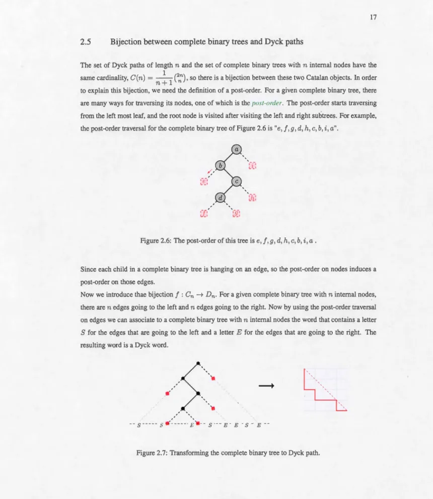
2.5 Bijection between

complete

binar

y

tree

s

and Dyck paths

The set of Dyck paths of length n and the set of complete binary trees with n internai nodes have the

sarne cardinality, C(n) = - 1- (2

n

)

,

so there is a bijection between these two Catalan abjects. In order

n+

1 n

to explain this bijection, we need the definition of a post-order. For a given complete binary tree, there are many ways for traversing its nodes, one of which is the post-orcier. The post-order starts traversing from the left most leaf, and the root node is visited after visiting the left and right subtrees. For example,

the post-order traversa! for the complete binary tree of Figure 2.6 is "e,

f

,

g, d, h, c, b, i, a".

,-ro '-'-'

'

~:

Figure 2.6: The post-order of this tree ise,

j

,

g, d, h, c, b, i, a.

Since each child in a complete binary tree is hanging on an edge, so the post-order on nodes induce a post-order on those edges.

Now we introduce thae bijection

f :

Cn

-+

D

n.

For a given complete binary tree with n internai nodes,

there aren edges going to the left and n edges going to the right. Now by using the post-order traversa!

on edges we can associate to a complete binary tree with n internai nodes the word that con tains a letter

S

for the edges that are going to the left and a letter

E

for the edges that are going to the right. The resulting word is a Dyck word .

.

--- S ---S

-

~----

· ~

·--

S ·--E. E. S- E

(36)

18

We can ob tain a Dyck pa th by translating S'sand E's respectively into ou th and ea t steps. For example, Figure 2.7 shows the Dyck path of length four thal is obtained from the complete binary tree with four internai nodes (we have shown its post-order traversai in Figure 2.6). Our inverse bijection

f

-

1 _:_D_n_~

Cn, is recursive! y constructed with two cases as follows. Consider two Dyck paths of Figure 2.8:

SSEESSEE SSESSEEE

Figure 2.8: Dyck path which meets the diagonal (left one), and does not meet the diagonal (right one).

The first Dyck pa th can be broken into two sm aller Dyck paths, S SEEISSEE, at the point that the pa th meets the diagonal y=

-x+

4

(except the points (

4 ,

0 )

and

(

0 ,

4))

. H

owever, for the second Dyck pa th,

there is no such a breaking point.

Case

1. The given Dyck path meets the diagonal y

=

-x+

na

t

point except

(n,

0 )

and

(

0 ,

n)

.

So

the Dyck path breaks into two smaller Dyck paths on the meeting point. In each smaller Dyck palh by translating the S's and E's to left and right edges, we obtain the complete binary tree that correspond

to then1. Now· in arder to püt them togeû~er, we attach the root of the first tree to the left most leaf of

the second tree. If there is more than one break point, the algorithm continues recur ive! y. For example,

Figure 2.9 mentions that we can break SESE into two Dyck path such as SEISE. So by putting the rootofthe tree

f

-

1_(SE)_o_{n th}_e_l_eft_l_eafof_th_e_tr_ee

_f

_-

1_(SE),_wege_{t th}_e_tr_ee

_f

_-

1_(SESE).

root

~

A

··S············E·

_---+

.. ','··· E·

(37)

19

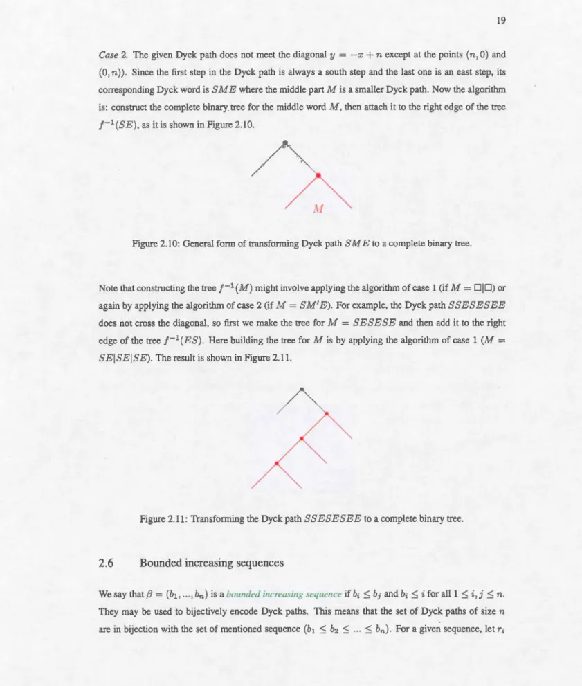
Case 2. The given Dyck path does not meet the diagonal y = -x+ n except at the points (n, 0) and

(0, n)). Since the first step in the Dyck path is always a south step and the last one is an east step, its corresponding Dyck word is SM E where the middle part M is a smaller Dyck path. Now the algorithm i : construct the complete binary. tree for the middle word M, then attach it to the right edge of the tree

f

-

1₍_SE₎_,_a _it_i_{s shown i}_n_{Figure 2.}₁₀_.

M

Figure 2.10: General form of transforrning Dyck pa th SM E to a complete binary tree.

ote that constructing the tree

f-

1

₍

_M

₎

_mi_g_ht_{involve a}_pplyin_{g the algorithm of case}₁_(if

_M

₌

_DIO₎_o_r again by applying the algorithm of case 2 (if M =SM' E). For example, the Dyck path SSESESEE

does not cross the diagonal, so first we make the tree for M = SESESE and then add it to the right edge of the tree f

-

1₍_ES)._H_ere_buildin_g_{the tr}_{ee for}_M _i_s_by_{applying the algorithm of case}₁_(M

₌

SEISEISE). The result is shown in Figure 2.11.

Figure 2.11: Transforming the Dyck path SSESESEE to a complete binary tree.

2.6 Bounded increa

s

in

g se

quence

s

We say th at ,8 = (b₁, ... , bn) is a bounded increasing sequence if b; :::; bj and b; :::; ifor ali 1 :::; i, j :::; n.

They may be used to bijectively encode Dyck paths. This means that the set of Dyck paths of size n

(38)

20

be the number of times that i occurs in the sequence. Then we associate the following Dyck path to the sequence:

Tt T2 Tn

~~ ~

S ... S

E S ...

S

E ..

.

S

..

.

S

E.

Here,

S

denotes a south step (0, 1),

andE

denotes an east step (1, 0). For example, as Figure 2.12 shows,

the weakly increasing sequence 1:::; 1:::; 1:::; 3 COITe ponds to the Dyck path

SSSEESEE:

i = 1 r1 = 3

i= 2 r2 = 0

,...--.._,

r1=3 ~ 1'3=1

SSSEE

s

EE

i=3 r3 = 1 i=4 r4 = 0

Figure 2.12: Sequence (1, 1, 1, 3) -t Dyck path

SSSEESEE.

Our inverse bijection, is constructed as follows. For a given Dyck path, the length of i-th vertical run is the number of occurrences of i in the corresponding bounded increasing sequence. For example, for

the Dyck path of Figure 2.13,

eh)= 2

,eh) =

o

,e(ra)

= 1,e(r4 ) = 1. This means that in the

bounded increasing sequence 1 occurs two times, 2 does not occur, 3 occurs once, and 4 occurs once so corresponding sequence is 1134. lenght of r1 = 2 lenght of r2 = 0 lenght of r3 = 1 lenght of r4 = 1 r1=2 1·3=l r4=l ~~~ ( 1, 1' 3 ' 4 )

Figure2.13:

Dyckpath

SSEESESE

-t sequence(1,1,3,4) .

Let us denote by B

n

the set of su ch sequences, which is enumerated by tbe Catalan numbers. For instance in the following we show some bounded increasing sequences of length 1, 2, 3 and 4 that encode Dyck

(39)

B

1

=

{

(1)}

L

B

2 =

{(1,1),(1,2)} :

L

.

~

8

3 .

=

{(1, 1, 1), (1, 1, 2), (1, 1, 3), (1, 2, 2), (1, 2, 3)} B4

=

{

(1, 1, 1, 1), (1, 1, 1, 2), (1, 1, 1, 3), (1, 1, 1, 4), (1, 1, 2, 2), (1, 1, 2, 3), (1, 1, 2, 4), (1,1,3,3), (1,1,3,4),(1,2,2,2),(1,2,2,3),(1,2,2,4),(1,2,3,3), (1,2,3,4)} 21

There are more than 200 other such bijections between the farnilies of mathematical objects counted by Catalan numbers. Later in Chapter 5, we will see that the set of "maximal tubings of path graphs" is in bijection with the set of complete binary trees.

(40)

(41)

CHAPTERIII

TAMARI POSET ON CATALAN OBJECTS

In this chapter we introduce the notion of Tamari lattice, and two of its realizations. First as a poset on

complete binary a·ees, and thenon Dyck path . Furthermore, we explicitly describe the covering relation

for the families of Catalan abjects previously considered in Chapter 2. We also count the number of intervals of Tamari posets, by using the zeta polynomial to count the number of chains in the Tamari po set.

3. 1

Tamari po

s

et

One of the interesting lattices in combinatorics is the Tarnari lattice, introduced by Dov Tamari. Tamari in his thesis [14, 1951], considered the set of well-formed parentheses strings of teng th 2n with

n

open, and n closed parentheses such that each opening parenthesis has a uniquely associated closing parenthesis

at its right. For instance, the possible well-formed parentheses strings of length 6 with those condition are()()(),(())(),()(()),(()()),((())). Later in [15, 1962], he partially ordered this set with the covering

relation (

)

()--+

(()),in the right-to-left direction. This poset with the described relation is a lattice that is know as the Tamari lattice, denoted T,... The property that makes the Tamari lattice one of the most

controversial issues of combinatorics is its cardinality that is given by the n-th Catalan number:

Number of elements of

T,..

= - 1- (2n) . n+ 1 n

The e lattices possess realizations as special polytopes', called "associahedra", which appeared in Stash -eff's thesis in 1961. Thus the 1-skeleton 2 of the n-dimensional "associahedron" corresponds to the

Hasse diagram of

T,..

(see [10] for more details). For example, Figure 3.1 indicates the Tamari lattice

73

which has five elements.

1 _{A po}_l_ytope_i_{s a geometrie}_objec_t_w_i_t_{h fl}_at_s_{ides t}_h_a_t_exis_t_s_i_n_any_num_ber_of_di_m_e_n_sio_n_s.

(42)

24

( ( ( ) ) ) (( )( )) ( )(( )) (( ))() ( )()()

Figure 3.1: The Tamari lattice Tg .

There are many realizations of the Tamari lattice a a partial order on "Catalan objects". In thi chapter,

we will study the covering relations in posets of complete binary trees, Dyck paths, and Dyck words. It

is clear that, by the bijection between complete binary tJ·ees and Dyck paths, the Tamari lattice of one can be obtained from the other.

The first result about the intervals of the Tamari lattice (i.e. pairs [P,

Q]

such thaL P ~ Q for P, Q E

T,..)

was from Chapoton in [6]. He proved that intervals in the Tamari lattice are enumerating by the following

formula:

2 (4

n

+

1)

Number of Intervals of

T,..

=

(

)

,

nn+1 n- 1 (3.l.l)

which gives the following sequence:

1, 3, 13, 68,399, 2530, ... (see htlps:!/oeis.org A000260)

For example, for the Ta mari poset

Ts

in Figure 3.2, the number near each vertex is the number of intervals

with th at vertex the top of the interval. Renee the total number of intervals in

Ts

is 1

+

2

+

3

+

5

+

2

=

13

that satisfies equation (3.1.1) for n

= 3.

[A, A] [A,B],[B,B] [A,

CJ

,

[B, CJ, [C,

CJ

[A,D],[D,D] [A, E], [B, E], [C, E], [D, E], [E, E]

@

c

Figure 3.2: The enumeration of intervals in Tamari lattice

Ts

.

(43)

25

Also, we can calcula te the zeta polynomial by equation (1.2.1) for Tamari po sets. For instance we have

Zr,(n)

= 1.

Zr,(n)

=

1 +n

.

Zr, ( n)

=

n

+

3 (~)

+

(~).

Zr,

(n)

=

n

+

12 G)

+

29(~)

+

26(~)

+

11(~)

+

2(~).

Table 3.1 illustrates sorne values of the zeta polynomial for Tamari posets, denoted Z.r; (k). The second column of the table i the Catalan sequence which counts the number of multi-chains from

Ô

to Î of length two in each Tamari poset. The third column of table is the sequence 3.1.1 that counts the number of intervals of each Tamari.

I':Z

1 2 3 4 5

1

2

1

2

3

4

5

3

1

5

13

26

45

4

1

14

6

8

21

8

556

Table 3.1: Sorne values of the zeta polynomials for the Tamari posets

7i

,

72 ,

73 ,

and

T4 .

3.2 Ta mari po

se

t on

binary tree

s

The Tamari order on the poset of binary trees is rotation operation. As it is shown in Figure 3.3, if a complete binary tree

T

is composed of a root "•", and a left subtree "•", then the right rotation of ton

"•" means replacing

(A

• B)

• C

by

A

• (

B

• C)

in

T

(note that

A

,

Bo

r

C

might be empty). Hence, this is

associativi ty.

~c

A B B

c

(44)

26

Consider two complete binary trees

tt

and t2 of the same size. We say that t2 covers t1 in the Tamari

lattice if and only if t2 can be obtained by a sequence of right rotation from t1. Figure 3.4 shows this

notion.

~

x

~

:

c

:

~

\"

y

tl

~--'

:

t

2 f

A"

:

'

JE

-:

~

r

Ë4

'

_(Cl

~· l__,

L_l

~--' Figure 3.4: Notion of

_t1

~

t2

.

The set of complete binary trees of size

n

with the Tamari order is in fact a lattice. For example, Figure 3.5 shows the Tamari lattice for n

=

3 and n

=

4.

~

..

.

· ~

..

.

· ?

· .

.

--

...

·

· '

..-~

1 ...

·..

.

....

· ..

...

. ·· .

.

· ··

~

'\'·~

\

..- ....

·.

.

A

....

~

.

....

~

..

.

....

b

?

· .

/

..

.

···.•

..

.

,

..

<f

..

.

"

...

_.

.

~ " .. ·.

Figure 3.5: The Tamari lattice of complete binary trees for n

=

3 (left) and n

=

4 (right).

(45)

- - -- - -- - -- - - -- - - -- - -

-27

Sine complete binary trees correspond bijectively to binary trees, we clearly have an equivalent descrip -tion of Tamari lattice in terrns of the la ter. Th us we get the representations in Figure 3.6.

Figure 3.6: The Tamari lattice of binary trees

for n

=

3 (left) and n

=

4 (right).

3 .

3 Tamari po

se

t on

Dyck

path

s

Con si der two Dyck paths d1 and d2 of the same size. We say that d2 co vers d1 if and only if there exists

in d1 an east step

a,

and a south step b following

a,

such that d2 is obtained from d1 by swapping

a

and

F

,

where

F

i

s

the shortest factor of d1 that begins with

ban

d

is a Dyck path. Figure 3.7 shows this notion.

Figure 3.7: Notion of d1 ~ d2 .

(46)

28

represents the Tamari lattice for n = 3 and n

=

4.

Figure 3.8: The Tamari lattice of Dyck paths for

n

=

3 (left) and

n

= 4 (right).

3.4 Ta mari poset on

Dy

ck

words

Consider two Dyck words w1 and w2 of the same length. We say that w2 covers w1 if and only if there

exists in w₁a letter

S

following

E

,

uch that w2 is obtained by changing the place of

E

and

F

, where

F is the shortest tactor of w1 that begi.ns with S, and is a Dyck word. For example the two Dyck words

w1 =

SSSEESSEESEE

and w2

=

SSSESSEEESEE

,

which correspond to the Dyck paths of

Figure 3.5, illustrates the notion of w1 ~ w2 :

SSSE

E

§.§!}3

SEE

~

SSSE

§.§!}3

E

SEE.

F F

(47)

29

Clearly, one can transfer the poset structure from that on Dyck paths to any other Catalan family using an explicit bijection. Hence, for

D

n

as a set of Dyck paths and

C

n

as a set of other Catalan abjects, one sets

B(a)

:S

B

({J)

if and only if a

:S

fJ

for

a

,

fJ

E

D

n

,

and

B : Dn

--*

C

n

a bijection. However, a direct description of the arder on

C

n

is often preferred.

For example, let T be a triangulation of a polygon (which is counted by Catalan numbers) such as Figure 3.9. Within

T

,

the diagonal

t

is the diagonal of sorne quadrilateral. Then there is a new triangulation

T'

which is obtained by replacing the diagonal

t

with the other diagonal of tb at quadrilateral. This local move is called an edgeflip, and we say that T' is obtained from T by flipping the diagonal

t.

edge flip

-+

Figure 3.9: Two triangulations

T

and

T'

are being related by an edge flip.

This case is interesting since it plays a crucial role in the origin of the notion of "cluster algebras"(see [16] for more details).

Then the question emerges that,

ls there sorne systematic way to think about "flips" in the Tamari poset of Catalan abjects?

In Chapter 5, we are going to introduce what is the Tamari arder for the notion of "tubing", as a main goal of the current study.

(48)

(49)

CHAPTER IV

PARKING FUNCTIONS ON CATALAN

OBJECTS

In this chapter we introduce the notion of parking functions, and sorne of their properties. Here our interest is in associating parking functions to Catalan objects. Hence we can identify a parking function with a labeled Dyck path, Dyck word, and complete binary tree. The bijection between parking functions and labeled Dyck paths lead to the creation of labeled intervals in the Tamari lattice of Dyck paths. On the other hand, we try to enumerate parking functions with zeta polynomial.

4 .

1 Parkin

g

fun

c

tion

s

The notion of "parking function" was introduced by Konheim and Weiss. In [9], they proved that the number of parking functions of length n is

La ter, other combinatorialists gave sorne methods of counting the number of parking functions of length n, or introduced bijections relating parking functions to other combinatorial structures. The parking problem was described in [2] as the following story:

"Imagine a one-way street with n parking spots and a cliff at its end. We'll give the first parking spot number 1, the next one number 2, etc ... , and the last one number

n

.

At first ali of them are free and there aren cars on the street, and they would alllike to park. Every car has a parking preference, and we record the preferences in a sequence, for example, if n

=

3, the sequence (2, 1, 1) mean th at the first car would like to park at spot number 2, the second car prefers parking spot number 1, and the last car would also like to park at number 1. The street is narrow, so there is no way to back up. Now each three car in the street start to park on its preferred parking spot; if it is free, it parks there, and if not, it can goes to the first available spot. We cali a sequence a parking function (of length n) if ali cars fi nd a parking spot at the end and none fall off the cliff". For example, the sequence (2, 1, 1) is a parking function (of

Generalization of Catalan combinatorics to the context of graphs

-UNIVERSITÉ DU QUÉBEC À MONTRÉAL