OATAO is an open access repository that collects the work of Toulouse
researchers and makes it freely available over the web where possible
Any correspondence concerning this service should be sent
to the repository administrator:
[email protected]
This is an author’s version published in:
https://oatao.univ-toulouse.fr/26469
To cite this version:
Lechuga-Crespo, Juan-Luis and Sanchez-Pérez, José Miguel and
Simeoni-Sauvage, Sabine and Hartmann, Jens and Amiotte-Suchet,
Philippe and Probst, Jean-Luc and Ruiz-Romera, Estilita A model
for evaluating continental chemical weathering from riverine
transports of dissolved major elements at a global scale. (2020)
Global and Planetary Change, 192. 1-14. ISSN 0921-8181
Open Archive Toulouse Archive Ouverte
Official URL :
https://doi.org/10.1016/j.gloplacha.2020.103226
A model for evaluating continental chemical weathering from riverine
transports of dissolved major elements at a global scale
J.L. Lechuga-Crespo
a,b,⁎⁎, J.M. Sánchez-Pérez
a,⁎, S. Sauvage
a, J. Hartmann
c, P. Amiotte Suchet
d,
J.L. Probst
a, E. Ruiz-Romera
baLaboratoire Ecologie fonctionnelle et Environnement, Université de Toulouse, CNRS, INPT, UPS, Campus ENSAT, Avenue de l'Agrobiopole, 31326 Castanet Tolosan,
CEDEX, France
bDepartment of Chemical and Environmental Engineering, University of the Basque Country, Plaza Ingeniero Torres Quevedo 1, Bilbao 48013, Basque Country, Spain cInstitut for Geology, Department of Geosciences, Center for Earth System Research and Sustainability (CEN), Universität Hamburg, Bundesstraße 55, 20146 Hamburg,
Germany
dBiogéosciences, UMR 6282, CNRS, University of Bourgogne Franche-Comté, 6 boulevard Gabriel, Dijon F-21000, France
A R T I C L E I N F O Keywords: Empirical model Ionic flux Chemical weathering Global scale A B S T R A C T
This study presents a process-based-empirical model for the assessment of ionic fluxes derived from chemical weathering of rocks (ICWR) at a global scale. The equations are designed and the parameters fitted using riverine transport of dissolved major ions Ca2+, Mg2+, K+, Na+, Cl−, SO42−, and alkalinity at a global scale by com-bining point sampling analysis with spatial descriptions of hydrology, climate, topography, lithology and soil variables such as mineral composition and regolith thickness. Different configurations of the model are con-sidered and the results show that the previously reported “soil shielding” effect on chemical weathering (CW) of rocks presents different values for each of the ions considered. Overall, there is good agreement between median and ranges in observed and simulated data, but further analysis is required to downscale the model to catchment scale. Application to the global scale provides the first global ICWR map, resulting in an average cationic flux derived from chemical weathering of 734·106Mg·y−1, where 58% is Ca2+, 15% is Mg2+, 24% is Na+and 3% is K+, and an average anionic flux derived from chemical weathering of 2640·106Mg·y−1, where 74% is alkalinity, 18% is SO42−, and 8% is Cl−. Hyperactive and hotspot areas are elucidated and compared between ions.
1. Introduction
Freshwater chemical composition has long been used as a proxy to understand the processes occurring in a catchment (e.g.Gibbs, 1970; Amiotte Suchet and Probst, 1993a;Romero-Mujalli et al., 2019). The insights obtained from these analyses are relevant for assessing bio-geochemical cycles, since rivers are vectors of matter transport between land and oceans (Probst, 1992). Major ion riverine loads are linked to the mineralogical composition of the underlying bedrock and overlying soil, and to their sensitivity to chemical weathering (CW) (Hartmann et al., 2009). CW of rocks is the process responsible for transforming rock into saprolites and soils, i.e. soil pedogenesis, in the Critical Zone (CZ) (Riebe et al., 2017), which releases dissolved compounds that are subsequently transported by rivers.
For several decades, evaluation and quantification of CW has been the focus of hydrogeochemical research (Livingstone, 1963;White and Blum, 1995;Di Figlia et al., 2007;Jansen et al., 2010;Hartmann et al., 2014a;Raab et al., 2019) and in more recent years it has also been used to quantify trends in salt increases related to human activities (Meybeck, 2003;Moosdorf et al., 2011;Guo et al., 2015;Kaushal et al., 2018). Large-scale studies have focused CW analysis on its implications for atmosphere/land/ocean fluxes and the Earth's climate, in influen-cing the biogeochemical cycles of elements by regulating CO2
con-sumption, or nutrient release (Amiotte Suchet and Probst, 1993b; Amiotte Suchet and Probst, 1995;Dupré et al., 2003;Hartmann et al., 2014a). However, fewer studies have centred on individual ion analysis (e.g.Goddéris et al., 2006;Goddéris et al., 2009) and, to the authors' knowledge, there is no spatially explicit reference product for ionic
⁎ Corresponding author.
⁎⁎ Corresponding author at: Laboratoire Ecologie fonctionnelle et Environnement, Université de Toulouse, CNRS, INPT, UPS, Campus ENSAT, Avenue de l'Agrobiopole, 31326 Castanet Tolosan, CEDEX, France; Department of Chemical and Environmental Engineering, University of the Basque Country, Plaza Ingeniero Torres Quevedo 1, Bilbao 48013, Basque Country, Spain.
E-mail addresses: [email protected] (J.L. Lechuga-Crespo), [email protected] (J.M. Sánchez-Pérez).
biogeochemical cycle adopted in this study is shown in the Supple-mentary Information, Fig. S1.
Atmospheric deposition incorporates ions to the CZ (from above the ground through the soil and saprolite horizons to the bedrock,Keller, 2019) which are either concentrated in the soil surface by evapo-transpiration and washed out of the catchment through surface and sub-surface runoffs; or infiltrated into the saprolite down to the unsaturated and saturated zones, reaching the groundwater reservoir. Soil processes —such as organic matter decay and root uptake followed by biomass storage— interact with these salts and may present synergies with the transport fluxes, altering the concentration of the salts present in the lateral flow (or subsurface runoff) and subsequently the river water (Keller, 2019). As regards the groundwater source, salts are derived from water interaction with rocks and later transported to the stream with groundwater flow (or baseflow).
CW has long been reported as a dominant process in major water composition, and several studies (Garrels and Mackenzie, 1972;Stallard and Edmond, 1981;Velbel, 1993;Gaillardet et al., 1999;Balagizi et al., 2015) have highlighted the relevance of lithology, hydrology, soil chemistry, and temperature, as variables that condition both CW and soil processes, while distance to the coast and altitude mostly affect atmospheric deposition (Meybeck et al., 1986,Vet et al., 2014). The combination of all these variables, in addition to human input, condi-tion major ion loads leaving the catchment.
Other dissolved compounds may be found in the dissolved riverine loadings which may interact with major ions, such as SiO2, NO3−, or
PO43−. However, these elements have not been included within the
scope of the modelling, since their global biogeochemical cycles are more complex and more closely linked to biological interactions (c.f. Galloway et al., 2004,Hartmann et al., 2014a) than those of the major ions selected, which are assumed to have more similar pathways be-tween reservoirs and a more stable temporal evolution (Keller, 2019).
2.2. Workflow and data overview
In order to estimate the specific fluxes of major ions, i.e. Ca2+,
Mg2+, K+, Na+, Cl−, SO
42−, and alkalinity, linear regressions have
been developed using global databases as input data, fitting the para-meters of the equations to minimize the difference between modelled and observed data. The mathematical approach used to develop the equations and fit the parameters is based on previous literature (e.g. Meybeck, 1979;Amiotte Suchet and Probst, 1993a, 1993b;Hartmann, 2009).
The observed chemical concentrations used in this study were taken from the GLORICH database (Hartmann et al., 2014b, retrieved from https://doi.pangaea.de/10.1594/PANGAEA.902360), which compiles over 1.2 million analyses of river waters around the world, as well as containing additional information on the draining catchments at the sampling locations. In order to focus on sampling locations mainly af-fected by atmospheric deposition and chemical weathering fluxes, a subset of the samples was created (see Section 2.2.1). The specific chemical fluxes were derived from averaged chemical concentrations and specific discharge for each draining catchment, and the differ-entiation between the atmospheric and chemical weathering contribu-tion was computed using an independent dataset to estimate the at-mospheric deposition (see Section 2.2.2). Additional variables were then included in the analysis, such as soil type abundance taken from the Harmonized World Soil Database (HSWD,FAO et al., 2012), re-golith thickness (GSDE,Shangguan et al., 2017), and soil permeability (GLHYMPS,Huscroft et al., 2018). The incorporation of these databases is described inSection 2.2.3and a summary of the uncertainties may be found inSection 2.2.4. The workflow followed is shown in graphic form inFig. 1.
2.2.1. Data subset and estimation of atmospheric deposition
The original chemical data stored in the GLORICH HC was sorted to fluxes derived from chemical weathering of rocks (ICWR) at a global
scale that quantifies the natural rock fluxes of single ions.
Assessment of chemical weathering rates (CWR) at catchment-to-global scale has evolved over recent years due to improvements in la-boratory experiments, the compilation of river water chemical data-bases, and the development of technical resources in modelling (Meybeck, 1987; Amiotte Suchet and Probst, 1993a, 1995; Probst et al., 1994; Hartmann et al., 2014a; Perri et al., 2016; Dong et al., 2018; Biondino et al., 2020). A distinction can be drawn between two main approaches to hydrogeochemical modelling: mechanistic and empirical based models. On the one hand, mechanistic models such as WHAM (Tipping, 1994) or WITCH (Goddéris et al., 2006) base their calculation on distinguishing between several layers in the soil with different chemical weathering rates, integrating the chemical composition of soils and the drainage waters in a mass-balance where the dissolution of primary minerals is described through kinetic laws (Goddéris et al., 2006; Roelandt et al., 2010), though they require a large quantity of detailed data which is normally not available worldwide. On the other hand, empirical models relate CWR to environmental variables through linear and non-linear regression, using statistically fitted parameters (Meybeck, 1987; Amiotte Suchet and Probst, 1995; Dessert et al., 2003; Hartmann, 2009), ignoring the physical dynamics behind the process. Despite their greater degree of abstraction, empirical laws have ex-tensively been used to quantify global fluxes of matter (Hartmann et al., 2014a) and CO2 sequestration by rock weathering (Amiotte Suchet and
Probst, 1995; Probst et al., 1997; Dessert et al., 2003; Hartmann et al., 2009), since they require less exhaustive input data and fewer com-puting resources while at the same time providing a useful product.
Given that, to the best of the authors' knowledge, there are no spatially explicit results at a global scale for the contribution of each major ion to the total CWR, and that this needs to be quantified before assessing the global anthropogenic inputs of major ions (Vörösmarty et al., 2010),the present study seeks to develop and apply an empirical model at a global scale to quantify the ICWR of major elements. The methodology pursued is based on that presented by Hartmann et al. (2009), and the objectives are: i) to present the methodology used to develop a spatially explicit empirical model of ICWR; ii) to evaluate the limitations of this methodology and of application of the model; and iii) to present and contrast the preliminary results of the model at a global scale, including a discussion of spatial distribution and an assessment of hyperactive and hotspot areas.
2. Materials and methods
2.1. Conceptualization
Conceptualization of the CW process used in developing this model is explained in the following lines and shown in graphic form in the Supplementary Information, Fig. S1. Major ion fluxes — i.e. Ca2+,
Mg2+, K+, Na+, Cl−, SO
42−, and alkalinity (HCO3− + CO32−)— in
rivers have previously been used as a proxy of all the processes oc-curring in the upstream draining catchment (Garrels and Mackenzie, 1972; Meybeck, 1984, 1986; Hartmann and Moosdorf, 2011), and are also considered in the present study. Two sources are established with regards to the spatial unit of the catchment: allochthonous, when the origin of the element lies outside the boundaries of the catchment (i.e. atmospheric dry and wet deposition); and autochthonous when the source of the element lies within the catchment area (i.e. bedrock chemical weathering). Human activity is a third source of ions in rivers, which may be: allochthonous when ions originating from anthropogenic activities are brought to the river by atmospheric deposition, e.g. acid rain (Schindler, 1988; Likens et al., 1996; Mahowald et al., 2011); or
autochthonous when there are spot saline sources or diffuse input within
the unit, such as effluents from wastewater treatment plants (Carey and Migliaccio, 2009), cropland fertilization, or road salting (Moore et al., 2008; Dailey et al., 2014). The conceptual schema of the major ion
exclude samples with missing data for Ca2+, Mg2+, K+, Na+, Cl−,
SO42− or alkalinity, samples showing an ionic charge balance error
over ±10% and sampling locations with <3 samples. Around 65% of the original 1,274,102 samples analysed in 18,897 locations between 1942 and 2011 were excluded. Chemical concentrations at the sampling location were aggregated through the median value since the dis-tribution was non-normal according to a Shapiro-Wilk test (p < 0.01). Not all sampling locations presented an associated draining catchment, and some were nested catchments; these were also excluded, resulting in 1751 catchments ranging from 1 to 2.9·104 km2, with 3 to 1220
samples, depending on the catchment. A map showing the selected sampling locations and associated areas may be seen inFig. 2.
2.2.2. Estimation of derived variables and atmospheric deposition
Due to the heterogeneity of the data on the number of samples in each sampling location and the frequent lack of instantaneous dis-charge, average riverine specific fluxes, Fxmeasured in mol·m−2·y−1,
were estimated from riverine concentration and specific runoff (com-puted as the discharge at the outlet of the catchment divided by the draining area,Fekete et al., 2002) using Eq. 1. In this equation, specific runoff, qann, measured in mm·y−1, was multiplied by the average
con-centration Cxof the sampling location, measured in mol·L−1, for each
ion x.
Fx=qann·Cx (1)
Riverine-specific fluxes include the mass departing the catchment from bedrock weathering, atmospheric deposits and other sources (in-cluding anthropogenic activities). In order to estimate ICWR, it was necessary to subtract the contribution of atmospheric deposition (Meybeck, 1983). Anthropogenic input could not be quantified since the extent of the anthropic influence differs between catchments; it was therefore assumed to be negligible for major cations and anions at the scale of application. However, further research on the impact of human pressure is needed (Vörösmarty et al., 2010).
Atmospheric flux was estimated using the results ofVet et al. (2014) (HTAP database) on atmospheric seasalt and sulphur deposition. First, the mean seasalt flux throughout the catchment was computed for each catchment using the “raster” package in R (Hijmans, 2019). In order to
distinguish the contribution of each ion in the total salt deposition, an ionic concentration distribution profile was then calculated for coastal and continental zones in each continent. To compute these profiles, the raw data used inVet et al. (2014), obtained from the World Data Pre-cipitation Chemistry website ( http://wdcpc.org/global-assessment-data) was classified by continents and into coastal/continental, based on distance from the coast. Average concentration values and ratios to the total salt concentration were then computed (see chemical dis-tribution profiles in Supplementary Information Fig. S2 and Table S1). Once the percentages of each element within the total concentration were obtained, the catchments were classified into zones according to the position of their centroid. This classification, together with the mean seasalt deposition flux, allowed us to quantify the specific at-mospheric flux for each element in each catchment. CW fluxes were computed by subtracting the atmospheric deposition flux from the riverine flux.
2.2.3. Database integration
Spatial analysis was performed using ArcGIS 10.4 and mainly con-sisted of summarising raster files in the polygonal shapes of the draining catchment. All data was integrated using R software (R Core Team, 2018). Three worldwide databases were included in the original GLORICH catchment properties (CP) database. For each catchment, the cover percentage of each HSWD soil type (FAO et al., 2012) was computed, and the mean regolith depth (Shangguan et al., 2017) and mean hydraulic conductivity (Huscroft et al., 2018) were then sum-marised. The spatial resolution is different for each database included; the catchment borders were delimited using the Hydro1K database (c.f. Hartmann et al., 2014b) at a 30 arc-second resolution, the same as for the HWSD soil type database (FAO et al., 2012) and hydraulic con-ductivity (Huscroft et al., 2018). However, finer resolution is found for the global soil depth database (Shangguan et al., 2017). Uncertainties in dataset collection are discussed inSection 2.2.4. However, considering the global approach of the study and the relatively small size of some catchments (see Supplementary Information, Fig. S2), the spatial re-solution of the global databases was considered sufficient to represent the lithological and soil compositions, average soil depth, and hydraulic conductivity. GLORICH HC GLORICH CP HTAP GSDE GLHYMPS 2.0 sample sort aggregation GLORICH CP* correction CP calibration HWSD relative area calculation aggregation model configuration EQUATIONS parameter fit
model evaluation COEFFICIENTS CP validation
Fig. 1. Workflow summary. The green rectangles represent the original databases included in the analysis, while the yellow boxes contain the datasets derived for the
present analysis, and the arrows describe actions. The acronyms refer to: the GLORICH database (Hartmann et al., 2014b) which contains information on hydro-chemical analyses (HC) and catchment properties (CP); the Harmonized World Soil Database (HSWD,FAO et al., 2012); the global regolith thickness (GSDE,
Shangguan et al., 2017); the soil permeability (GLHYMPS 2.0,Huscroft et al., 2018); and the world precipitation chemistry dataset (HTAP,Vet et al., 2014). (For interpretation of the references to colour in this figure legend, the reader is referred to the web version of this article.)
The data pre-process resulted in a database with over 180 variables, including chemical fluxes, morphological variables (i.e. altitude, area, slope, etc.), climate variables (monthly and annual temperature, pre-cipitation, windspeed, etc.), land covers (forest, agricultural, managed percentages, etc.), soil types (Leptosols, Cambisols, Nitisols, etc.), soil descriptors (regolith thickness, hydraulic conductivity, pH, etc.), and lithology (Metamorphics, Plutonics Acids and Basics, Carbonate Sedimentary, etc.). This dataset was used to explore the relationships, calibrate the parameters of the equations, and test the residuals of the model created to further define the model.
2.2.4. Database uncertainties
The development, calibration, and validation steps of an empirical model rely on the data used for its construction. In this study, several types of data from different sources were included, selected following an assessment of their quality. Among chemical collection datasets, the GLORICH database (Hartmann et al., 2014b) was chosen because it contained a larger amount of data located in a greater number of catchments. Moreover, it contains two types of data: spot data (related to the samples analysed in each river) and spatial data (relating to the physical description of the draining catchment). Spot data was gathered from different monitoring programs and scientific literature and tested Fig. 2. Original, subset, and classified sampling locations and draining catchments in the present study. Within the original GLORICH dataset (light grey), the darker
grey areas represent the selected draining catchments, for which the outlets are represented as red or black points depending on whether they have been used for calibration (n = 1313) or validation (n = 438), respectively. (For interpretation of the references to colour in this figure legend, the reader is referred to the web version of this article.)
Fx=qann·cx (M1)
Fx=qann· (L ·c )i xi (M2)
Fx=qann s·f (soil)·x (L ·c )i xi (M3)
Fx=qann T·f (temperature)· (L ·c )i xi (M4)
Fx=qann s·f (soil)·f (temperature)·x T (L ·c )i xi (M5)
Fx=qann D·f (soil depth)· (L ·c )i xi (M6)
Fx=qann K·f (hydraulic conductivity)· (L ·c )i xi (M7)
Fx=qann KD·f (soil depth+hydraulic conductivity)· (L ·c )i xi (M8)
f F F s x(shield 0.5) x(M2,shield 0.5) x= f exp 1 T 1 T T= f Depth Depth b·Depth D MAX = f K K b·K K hyd
hydMAX hyd
= f Depth K KD hyd =
where Fx⁎represents the ionic flux derived from chemical weathering of
rocks (ICWR) of an element x, measured in mol·m−2·y−1; q
ann
re-presents the annual average runoff composite of the catchment
(computed as the discharge at the outlet of the catchment over the area of the draining surface), in dm3·m−2·y−1; L
iaccounts for the percentage
of the area covered by a lithological group i (see Fig. S6); fs,xis the soil
shielding effect factor, dimensionless; fT represents the temperature
effect factor, dimensionless; fDis the soil depth factor, dimensionless;
and the fKconsiders the hydraulic conductivity factor, dimensionless;
fKDis the soil depth-hydraulic conductivity factor, dimensionless; Fx⁎M2
is the flux obtained with model M2, in mol·m−2·y−1; T is the average
annual air temperature of the draining basin taken from the GLORICH database, computed from the WordClim (Hijmans, 2019) database, in K; T is the global average annual temperature, in K; Depth measures the soil depth, in cm; and Khydmeasures the mean hydraulic conductivity,
in m·s−1. A further detail of the former three factors is set out in the
following paragraphs. For all models tested here, the parameters are cx,
cx,i, measured in mol·L−1, and b, dimensionless, and may be interpreted
as the average concentration of an element x in the water draining from rock i (cx and cx,i) corrected for atmospheric inputs, and b as the
function parameter. The parameters fitted at the calibration step are cx,
cx,i, and b.
Soil cover over bedrock has been identified as an important factor to consider when analysing the CW at a global scale (Dupré et al., 2003; Hartmann et al., 2014a). Some soil types with thick profiles, or high organic matter content, or low permeability may act as a buffer to the chemical flux arriving to the river stream, as shown byBoeglin and Probst (1998)for large river basins covered by lateritic soils, where the fluxes of bicarbonates supplied by silicate hydrolysis are half of the river fluxes produced in non-lateric basins. In this regard,Hartmann et al. (2014a)estimated an average soil shielding factor of 0.1 for the following FAO soil types: Ferralsols, Acrisols, Nitisols, Lixisols, Histo-sols, and Gleysols. Here, we consider a similar factor, but differentiating between the values for each ion. Further explanation is given inSection 2.4. In this study, 416 catchments showed a percentage of coverage of this kind of soil of 50% and were expected to be affected by the “soil shielding effect”.
In order to include the soil shielding effect fs,xwe established a
threshold to differentiate between two groups of catchments: those in which 50% or more of the area was covered by the sum of the soil types Ferralsols, Acrisols, Nitisols, Lixisols, Histosols, and Gleysols (Hartmann et al., 2014a), where the dominance of the soil shielding effect was expected; and those where this sum was under 50%. The mean values of the flux for each group and ion was computed and the ratio of atmo-spherically corrected observed flux to flux obtained with model M2, for soil-shield-affected affected catchments was computed, giving fs, Ca2+ = 0.75; fs, Mg2+= 0.74; fs, Na+= 0.46; fs, K+= 0.78; fs,
Alkali-nity= 0.70; fs, SO42−= 0.29; fs, Cl−= 0.34.
As regards the temperature effect, catchments with higher average temperature were expected to drain higher fluxes of elements than those with lower temperatures. Annual air temperature was used as a proxy for groundwater mean temperature, which is that responsible for changes in the solubility constants of certain minerals. Then, a similar temperature factor toHartmann et al. (2014a)with an Arrhenius type equation was then computed as fT.
2.3.1. Calibration and model evaluation
The parameters from the equations were fitted using a 75% random subset of the data (ncalibration= 1313) from the selected sites (Fig. 1),
while the remainder were used for validation (nvalidation= 438). The fit
was carried out using the Levenberg-Marquardt algorithm, a method used to find the minimum of a function, in this case, a sum of squares (Moré, 1978), implemented in the “minpack.lm” package (Elzhov et al., 2010) for the R software (R Core Team, 2018). As the parameters to fit were interpreted as the concentration (cx, cx,i) of an element draining
from water from each lithological group, a lower boundary of 0 was established. The performance of the model was evaluated by assessing the significance of the relation between observed and simulated values using Spearman correlation (ρ) and evaluation of the percentage of to eliminate possible errors, although this dataset was considered to
have been validated by its creators (Hartmann et al., 2014b). The spatial data for both the GLORICH description of the draining basin characteristics and the added variables is based on contrasted spatial datasets. The lithological distribution was taken from the Global Li-thological Map (GLIM, Hartmann and Moosdorf, 2012) which, to the best of the authors' knowledge, is the highest resolution lithological database at a global scale. Soil type abundance was computed using the polygons in the Harmonized World Soil Database (HSWD, FAO et al., 2012). The hydrology was taken from the 0.5°x0.5° raster in the UNH/ GRDC Composite Runoff F ields V 1.0 (Fekete e t a l., 2 002). Regolith thickness was taken from the 1x1km raster Global Soil Regolith Thickness (GSDE, Shangguan et al., 2017). Hydraulic conductivity was estimated from the polygons in Global Hydrogeology Maps (GLHYMPS, Huscroft et al., 2018). The seasalt atmospheric deposition was derived from 1°x1° raster from the global assessment of precipitation chemistry (Vet et al., 2014). The uncertainties and limits for each dataset are set out in each of the publications, while in the present analysis the global results are modelled (using the soil, lithology, and specific runoff da-tabases) at a resolution of 0.5°x0.5°.
2.3. Modelling approach
Chemical weathering rates are mainly affected b y h ydrology, li-thology of the underlying bedrock, the overlying soil, and water tem-perature (Hartmann et al., 2009; Hartmann et al., 2014b). In order to analyse the effect of each one on all of the ion fluxes, it was proposed to test 8 linear equations. To design the equations, a physical interpreta-tion of the estimates was considered, and the variables were added in the following order: lithology, soil shielding effect (further explained in the paragraphs below and in Hartmann et al., 2014b), temperature, hydraulic conductivity and soil depth. The set of equations tested is as follows:
deviation (PBIAS), which measures the average tendency of the simu-lated values to be above or below the observed values.
cov(rg , rg ) ; PBIAS (F F ) F Observed Simulated rg rg Simulated Observed Observed Observed Simulated = =
where cov(rgObserved,rgSimulated) is the covariance of the observed and
simulated fluxes, σrgrepresents the standard deviation of the variables,
and F represents the specific fluxes. Finally, the model is applied over a grid with a cell size of 0.5 × 0.5° where superposition of the GLiM, HSWD, and UNH/GRDC (Fekete et al., 2002) datasets allowed for the generation of single combination cells where the M3 model estimates were applied.
3. Results
3.1. Assessment of model performance
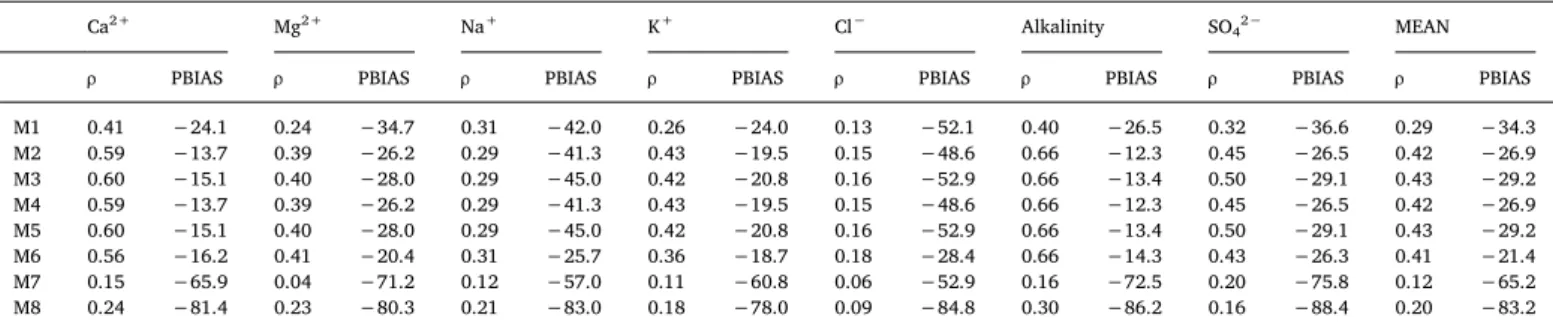
Table 1summarises the statistics used to evaluate performance of the model, all of which show a significant correlation (p < 0.01). M1 only includes the average specific runoff and the fitted parameter re-presents the average concentration of element x in all catchments; it is used here as a starting point for model performance. As expected, the inclusion of lithology in theregression (M2)improved correlation of the model and decreased the difference between observed and simulated data. Inclusion of the “soil shielding” effect (M3) therefore has im-proved the correlation but also increased the difference between the data, as shown by the increase in PBIAS. The incorporation of tem-perature (M4) had no effect when compared to model M2, and neither did the combination of “soil shielding effect” and temperature (M5), while aggregation of soil depth (M6) decreased the correlation with regard to M2 and M3. M7 and M8 show the lowest correlations and the highest PBIAS. It is important to note that there are almost no differ-ences in the statistics from M2 to M5, although the best performance of the model, with the fewest explanatory variables, was achieved with M3, as further analysed in this study.
In general, there is a strong and significant correlation between the median observed and simulated values considering all catchments and ions included in the present study (rSpearman= 0.96, p < 0 .01), as
shown inFig. 3. In addition, both observed and simulated fluxes expand over similar interquartilic ranges (IQR = 3rdQ-1stQ), suggesting that
this model configuration is capable of estimating the median and ranges of ionic-specific fluxes in large scale studies.
When each ion is evaluated independently, and site-specific fluxes are compared in observed-simulated pairs, two findings may be de-rived: there is a higher data scatter, as shown by lower ρ and a greater underestimation of the model, noted by a more negative PBIAS (Table 1). For M3, the best represented ions are Ca2+and Alkalinity,
with correlations of over 0.6 and a PBIAS of under 15%, while the poorest are Na+ and Cl−, with correlation of under 0.3 and PBIAS
>45% (Table 1). Nevertheless, the residuals display a normal dis-tribution, centring on 0, suggesting a valid model configuration.
Application of the model to the validation dataset gives the result shown inFig. 3b. Like the calibration dataset, the model shows better results for alkalinity, and worse results for Cl−.
3.2. Application of the model
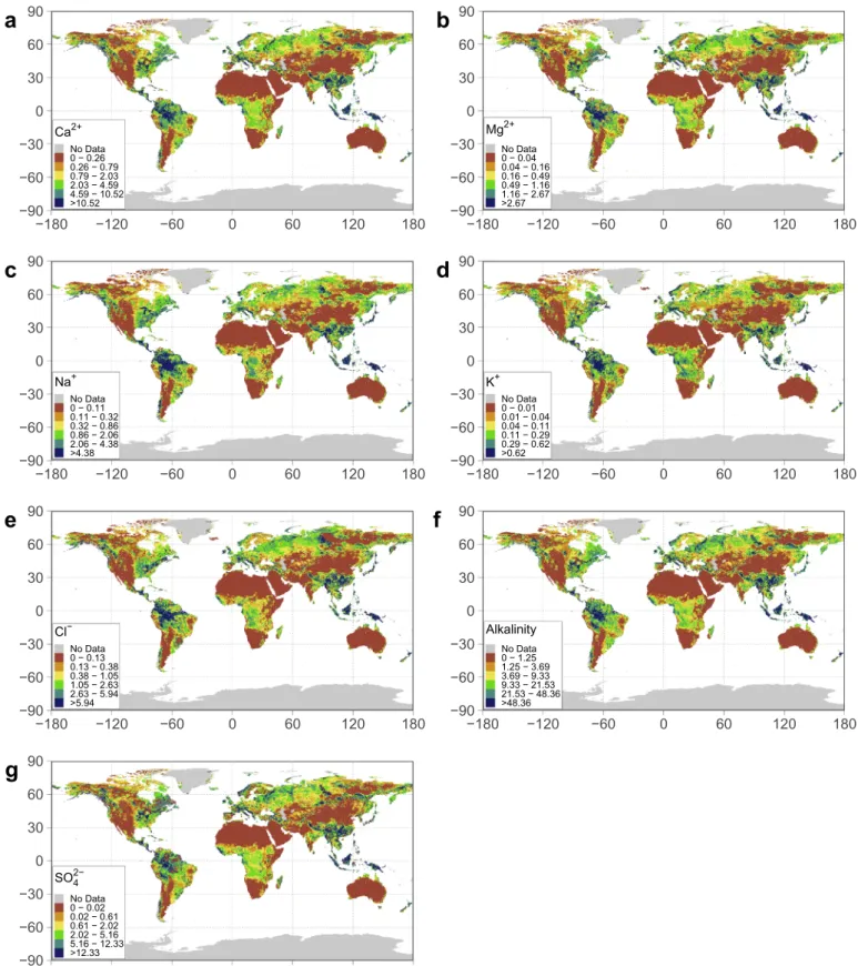
Model M3 has been considered to represent a fair starting point for assessing ICWR at large scales. Before applying it to smaller case stu-dies, it should be contrasted in specific case studies with adapted data, such as observed average specific discharge, soil maps, and lithological distribution, with a finer resolution, instead of using globally derived products. Here, the model is applied to a grid with a cell size of 0.5° where superposition of the GLiM, HSWD, and UNH/GRDC datasets al-lowed for the generation of single combination cells in which the M3 model estimates were applied. The results of this application are dis-played in Fig. 4, which shows the spatial distribution of the ICWR, measured in Mg·km−2·y−1for easier comparison with previous studies
inTable 2.
Overall, higher ICWRs are obtained for alkalinity, SO42−, and Ca2+,
in concordance with the dominant elements commonly found in freshwater environments, while the lowest ICWRs are found for K+,
which commonly accounts for a lower proportion of water chemistry. In general, higher ICWRs are found in latitudes between 15° S and 15° N for all ions, probably related to higher specific discharge and humid tropical climates. This is clearly shown for alkalinity, presenting highest values for the Amazon and the Congo basins, as well as the Polynesian Islands. Low median fluxes are found between 15° N and 30° N and 15° S and 30° S but probably affected by the Saharan and Australian deserts, in contrast, the south-eastern parts of Asia and Central America show higher ICWR. In this study, relevant fluxes are also found between 45° N and 75° N whose contribution to chemical fluxes had previously been assessed as not being relevant (Hartmann et al., 2014a). In the GLORICH database and other input datasets, there is no catchment in the Antarctic and Greenland, though ICWRs in these areas are displayed as No Data, but they are probably affected by snow and ice processes not properly represented in this study, as described byWadham et al. (2010)andSt Pierre et al. (2019).
4. Discussion
4.1. Overall
The present study shows the development of an inverse model for the assessment of ICWR at a global scale, based on aggregated chemical analysis of spot samples at a catchment level around the world, as well as on worldwide datasets. It is the first time that a map of the ionic flux derived from chemical weathering of rocks is presented, and represents an improvement on previously published similar models (Meybeck,
Spearman correlation coefficients and PBIAS values [%] for the eight models tested here (M1-M8, n = 1313) in the calibration dataset. The last column (“MEAN”) shows the mean value for all ion assessment in each model. All correlations are statistically significant (p <0.01). M3 is considered the best and analysed further in this text.
Ca2+ Mg2+ Na+ K+ Cl− Alkalinity SO
42− MEAN
ρ PBIAS ρ PBIAS ρ PBIAS ρ PBIAS ρ PBIAS ρ PBIAS ρ PBIAS ρ PBIAS
M1 0.41 −24.1 0.24 −34.7 0.31 −42.0 0.26 −24.0 0.13 −52.1 0.40 −26.5 0.32 −36.6 0.29 −34.3 M2 0.59 −13.7 0.39 −26.2 0.29 −41.3 0.43 −19.5 0.15 −48.6 0.66 −12.3 0.45 −26.5 0.42 −26.9 M3 0.60 −15.1 0.40 −28.0 0.29 −45.0 0.42 −20.8 0.16 −52.9 0.66 −13.4 0.50 −29.1 0.43 −29.2 M4 0.59 −13.7 0.39 −26.2 0.29 −41.3 0.43 −19.5 0.15 −48.6 0.66 −12.3 0.45 −26.5 0.42 −26.9 M5 0.60 −15.1 0.40 −28.0 0.29 −45.0 0.42 −20.8 0.16 −52.9 0.66 −13.4 0.50 −29.1 0.43 −29.2 M6 0.56 −16.2 0.41 −20.4 0.31 −25.7 0.36 −18.7 0.18 −28.4 0.66 −14.3 0.43 −26.3 0.41 −21.4 M7 0.15 −65.9 0.04 −71.2 0.12 −57.0 0.11 −60.8 0.06 −52.9 0.16 −72.5 0.20 −75.8 0.12 −65.2 M8 0.24 −81.4 0.23 −80.3 0.21 −83.0 0.18 −78.0 0.09 −84.8 0.30 −86.2 0.16 −88.4 0.20 −83.2 Table 1
1987;Amiotte Suchet and Probst, 1995;Gaillardet et al., 1999;Ludwig et al., 2011;Hartmann et al., 2014a). In order to discuss the results, three main points are established:
•
A comparison is made between the results of the model and the last model presented on Chemical Weathering Rates (CWR, Hartmann et al., 2014a) and other global studies, in order to validate the re-sults obtained and contrast the differences.•
A framework of application of this model is established with regard to the spatial scale of application. In addition, the advantages that this configuration poses for potential users, and limitations re-garding scales and conceptualization are also discussed.•
An identification and comparison of the hotspots among ions at a global scale is described, to highlight the role of ICWR in global biogeochemical cycles.4.2. Model validation
The results of the present study are compared to previous studies in Table 2, considering the individual ionic fluxes and their aggregations in cation, anion and total fluxes. In general, the M3 model presents an average global CWR of ~3374·106Mg·y−1, which is lower than
pre-vious studies, e.g. ~4175·106 Mg·y−1 (Meybeck, 1979),
~4050·106Mg·y−1(Probst, 1992), but higher than more recent results
~2131·106Mg·y−1(Gaillardet et al., 1999). However, focusing
speci-fically on the ~734·106Mg ·y−1total cation flux (ΣZ+), it has a lower
value than a recent study at the same scale ~1439·106 Mg ·y−1
(Hartmann et al., 2014a). Differences in this result are attributed to three main causes: differences in the definition of CWR (inclusion of dissolved silica), the number and location of the reference sampling sites selected for the model calibration step, and the configuration of the model itself. According to results fromMeybeck (1979)andProbst (1992), the SiO2/Ca2+ratio is ~0.7, which would yield a ΣZ+M3⁎ of
~1034·106Mg·y−1closer to, but lower than, the study byHartmann
et al. (2014a).
The CWR measurement shows discrepancies between research stu-dies, given that several compute the total weathered matter from rocks through Total Dissolved Solids, TDS (e.g.Dessert et al., 2003;Donnini et al., 2016) while others make different aggregations, i.e. cations (e.g.
Gaillardet et al., 1999; Dessert et al., 2003;Balagizi et al., 2015) or cations plus SiO2(e.g.Hartmann et al., 2014a). In the present study,
each ion is computed independently to overcome these discrepancies, in a similar way toBraun et al. (2005)andGoddéris et al. (2009). Among the applications of these studies, a knowledge of CWR is of interest in assessing CO2consumption through rock dissolution (Amiotte Suchet
and Probst, 1995;Amiotte Suchet et al., 2003;Hartmann et al., 2009), in studying the global biogeochemical cycles of P (c.f.Hartmann et al., 2014a), and in characterising the riverine end-member in oceanic as-sessments (Sun et al., 2016). Assessing each ion independently offers an opportunity for a more detailed description of the CW process and the associated assessments at a global scale. In this regard, the present study will be a reference for future works, especially in large-scale applications (see discussion sections below). The ICWR model yields similar flux median and ranges values as compared to the observed data for alkalinity, but a poorer representation of Cl−, linked to a
pre-dominantly atmospheric input and traces of evaporites located in other lithological groups that are not large enough to be mapped at a global scale but are large enough to have a significant impact on riverine loads.
Previous authors have attributed the overestimation of empirically-modelled CWR in tropical areas (such as the Amazon, Congo, and Orinoco basins) and its underestimation in northern latitudes to the small number of sampling locations included in development of the model (see discussion inHartmann et al., 2014aandGoddéris et al., 2006). The recent study byHartmann et al. (2014a) extrapolated a regionally fitted model (using 381 sampling locations in the Japanese Archipelago, seeHartmann and Moosdorf, 2011) to the world, and further refined its formulation by considering 49 large river catchments in different locations worldwide, among which there are several tro-pical and Arctic basins. Gaillardet et al. (1999), on the other hand, initially included this kind of basin in their model fitting, taking the 60 largest rivers in the world as a reference. Here, 1313 sampling locations in large basins and small catchments in warm and cold climates around the world were used for the model fit step, reflecting greater variability in the parameter estimates and thus giving to more robust results, as supported by the residual normal distribution.
Nevertheless, even though the number of sampling locations is greater than in previous empirical model developments, they are Fig. 3. Scatterplot of simulated and observed data for calibration and validation, using model M3. Each point represents a median value for each ion considered in
spatially clustered in some areas, excluding relevant areas from the calibration and validation steps (Fig. 3). Northern latitudes (the Arctic catchments), Polynesian sampling locations and a large quantity of data available from Asia are not included in the present analysis because of
non-availability in the data source selected, or due to the subset cri-terion established (seeSection 2.2.1). Despite not including these areas, the calibration subset is considered to be representative of different climates, soils and lithological characteristics (see Supplementary
−90
−60
−30
0
30
60
90
−180
−120
−60
0
60
120
180
Ca2+ No Data 0 − 0.26 0.26 − 0.79 0.79 − 2.03 2.03 − 4.59 4.59 − 10.52 >10.52a
−90
−60
−30
0
30
60
90
−180
−120
−60
0
60
120
180
Mg2+ No Data 0 − 0.04 0.04 − 0.16 0.16 − 0.49 0.49 − 1.16 1.16 − 2.67 >2.67b
−90
−60
−30
0
30
60
90
−180
−120
−60
0
60
120
180
Na+ No Data 0 − 0.11 0.11 − 0.32 0.32 − 0.86 0.86 − 2.06 2.06 − 4.38 >4.38c
−90
−60
−30
0
30
60
90
−180
−120
−60
0
60
120
180
K+ No Data 0 − 0.01 0.01 − 0.04 0.04 − 0.11 0.11 − 0.29 0.29 − 0.62 >0.62d
−90
−60
−30
0
30
60
90
−180
−120
−60
0
60
120
180
Cl− No Data 0 − 0.13 0.13 − 0.38 0.38 − 1.05 1.05 − 2.63 2.63 − 5.94 >5.94e
−90
−60
−30
0
30
60
90
−180
−120
−60
0
60
120
180
Alkalinity No Data 0 − 1.25 1.25 − 3.69 3.69 − 9.33 9.33 − 21.53 21.53 − 48.36 >48.36f
−90
−60
−30
0
30
60
90
−180
−120
−60
0
60
120
180
SO42− No Data 0 − 0.02 0.02 − 0.61 0.61 − 2.02 2.02 − 5.16 5.16 − 12.33 >12.33g
Fig. 4. Holospheric distribution of Ionic fluxes derived from Chemical Weathering of Rocks (ICWR), all data expressed in Mg·km2·y−1. The maps were obtained by applying the model to a global grid of 0.5° using the fitted parameters in model M3. Note that each ion presents a different colour range based on the global percentile distribution, using P10th, P25th, P50th, P75th, and P90thas breakpoints.
Information, Figs. S3-S7), allowing a flexible tool to be developed that is capable of capturing a great variability in catchment characteristics, albeit acknowledging its limitations (seeSection 4.3Domain of appli-cation).
CW of rocks is a complex process that is controlled by several factors that vary with soil depth, e.g. the composition of minerals (Apollaro et al., 2019; Biondino et al., 2020), and the hydrology (Gabet et al., 2006; Anderson et al., 2004; Hartmann, 2009). Boeglin and Probst (1998) showed that for large river basins, the atmospheric/soil CO2
consumed by silicate weathering and the associated bicarbonate river fluxes are 1.8 times lower when the bedrock is covered by deep lateritic soils.Oliva et al. (2003)noted that regolith depth shields the rocks from CW in areas where this layer is thicker, howeverDong et al. (2018) reported that the highest CW occurs at an intermediate soil thickness. In this regard, we hypothesized that a larger regolith (soil+saprolite) layer would act as a proxy for erosion-product deposition, and in sy-nergy with a low hydraulic conductivity, would result in a lower CWR (Gabet et al., 2006;Anderson et al., 2004).
However, inclusion of global regolith thickness (Shangguan et al., 2017) and hydraulic conductivity (Huscroft et al., 2018) in this study did not improve the results. We associate this finding with the model configuration and the scale of application. In addition, the GLHYMPS database (Huscroft et al., 2018) was computed from the GLiM database, which is already accounted in the model variables, although informa-tion may already have been included in the lithological group classifi-cation. In contrast with our study,Dong et al. (2018)succeeded in in-cluding of these variables using a physically based model, by making a distinction between different soil layers. However, our data-driven model was not capable of including these variables within its context and the area of application poses a challenge in describing the required variables. Nonetheless, an improvement in performance of the model in relation to soil data can be found in the “soil shielding effect” factor (Dupré et al., 2003;Hartmann et al., 2014a), computed for soil types classified based on their pedogenesis in the HSWD database (FAO et al., 2012). Soils with thick layers, low hydraulic conductivities, dominated by organic matter decay, or with a shallow ground water table (Hartmann et al., 2014a) would have a stronger shielding effect. We attribute the improvement in the model's results to the soil shielding effect, and the lack of success in including new variables to the fact that the combination of the lithological and soil classification maps already takes into account the interaction of chemical fluxes with the soil layers overlying the bedrock zone, and the fact that the inclusion of regolith thickness and hydraulic conductivity requires a physically-based ap-proach for inclusion in studies of chemical weathering studies.
Temperature is another variable initially considered to be relevant in CW (Drever and Zobrist, 1992,Dessert et al., 2003, Hartmann et al., 2014), since it reflects changes in the equilibrium constant of the dis-solution reactions (Drever, 2012). An increase in water temperature would increase dissolution of rocks and augment biological activity, through respiration and pCO2in the soil, but it would also reduce the
gas dissolution in the liquid. However, CO2is produced by ecosystem
respiration, inducing acids responsible for chemical weathering; this is a two-factor dependence (soil water content and temperature) which explains why an Arrhenius-type factor for the model alone does not improve the results (Romero-Mujalli et al., 2019). Dissolution takes place in the regolith water and groundwater but we could find no da-tabase with worldwide spatially distributed temperature values. For this reason, air temperature is used as a proxy for this effect, but its inclusion does not provide any improvement in the model. This is re-lated to two main factors: the different effect on the dissolution of each mineral and that the fact that, although groundwater temperature is dependent on annual average air surface temperature, this variable appears not to be a proxy related to the temperature effect on CW re-actions. Further research is needed to analyse the effect of water tem-perature on these fluxes worldwide.
At the conceptualization stage (see Section 2.1), several other variables were considered, such as vegetation (land cover), evapo-transpiration, or a finer definition of rocks (including rock ages), but after some consideration, these data were not included in the devel-opment stage. Vegetation fixes atmospheric C through photosynthesis, which is later exchanged by roots with microorganisms during soil re-spiration, increasing the CO2 concentration in the soil pores, which
would dissolve in water to generate carbonic acid and enhance rock dissolution, thus releasing ions into the water matrix (c.f.Keller, 2019). However, changes in the photosynthesis process, soil respiration and evapotranspiration are processes with a higher variability (posing a challenge in modelling them, c.f.Chen and Liu, 2020) than the annual mean value used in this study, although this variability could not be captured. Evapotranspiration, conditioned by climatic variables such as temperature and precipitation, affects the water balance by extracting water from the system (i.e. basin) causing an increase in the saline concentration found in rivers. However, its effect on CW is less pro-nounced than other characteristics, such as lithological classification (White and Blum, 1995). This suggests that a better representation of the effect of precipitation, air temperature and other climatic variables on chemical weathering rates is mainly related to an improvement in the water balance at a basin scale, which could be achieved by using more detailed models. Lastly, in comparison with previous similar studies (Meybeck, 1986;Amiotte Suchet and Probst, 1995) recent stu-dies include a larger number of lithological classes (Hartmann et al., 2014b, this study), involving a finer definition of minerals. Despite this larger number, further levels of classification of lithologies are available (c.f.Hartmann and Moosdorf, 2012), but given the number of sampling locations, it would have been a challenge to include all of them, as most of them would not vary in a wide enough range to calibrate the para-meters in the model. Even with the classification used in this study, there are some lithological classes which do not span the entire spec-trum (e.g. plutonic intermediate, see Supplementary Information, Fig. S6), meaning that in the subset considered in this study, there are no catchments in which 100% of the draining area is covered by these lithologies. The inclusion of finer lithological classification should focus on smaller-scale cases, where mechanistic models may be applied, or Table 2
Comparison between studies on of CWR at global scales. All values expressed at 106Mg·y−1. ΣZ+represent the Ca2+, Mg2+, Na+, and K+while ΣZ−for Cl−, SO42−, and Alkalinity (expressed as HCO3−). Bracketed values represent a recalculation of ΣZ+adding a virtual contribution of SiO2, considering a SiO2/Ca2+of 0.7.
Study Code Ca2+ Mg2+ Na+ K+ Alkalinity SO
42− SiO2 Cl− ΣZ+ ΣZ− Total flux from Chemical Weathering
This study M1 374 100 223 25 1815 401 – 246 722 (984) 2462 3184 (3446) M2 484 121 202 29 2234 500 – 263 836 (1175) 2997 3833 (4172) M3 428 107 176 24 1954 465 – 221 734 (1034) 2640 3374 (3674) M4 527 132 221 31 2434 545 – 287 911 (1284) 3266 4177 (4550) M5 477 119 202 27 2139 490 – 241 825 (1159) 2870 3695 (4029) Meybeck (1979) Natural 502 126 192 48 1940 307 – 215 868 2462 3330 Total 549 136 270 53 2040 431 388 308 1008 3167 4175 Probst (1992) 510 141 211 73 2013 455 355 223 935 3046 3981 Gaillardet et al. (1999) – – – – – – – – – – 2131
Here, the present model defines the CWR by its constituents, i.e.
ions, analyses the weight of each one in the total flux and helps to assess the average specific flux. The poor representation of Na+ fluxes is
linked to different drivers governing the dissolution of the rocks with this kind of elements, such as albite or volcanic glass, which are re-ported as large CO2sinks in a global context (Dessert et al., 2003). In
order better to represent the Na+and SO
42− ions from an inverse
modelling point of view, other variables should be taken into con-sideration, as their presence may be linked more to redox processes than to congruent dissolution by acids (Berner and Berner, 2012), like dissolved oxygen concentration or redox potential, which are com-monly measured in the field. This finding highlights the importance of analysing all ions when considering CW and other associated processes, as since although the CWR has previously been quantified, the re-presentation of all ions in this flux is not equally well defined, in-dicating that further research is needed to improve the representation of those elements and an understanding of the associated processes. Keller (2019)shows an analysis of the Critical Zone and explains CW in its context; a relevant number of variables are tied up with this process (including denudation rate, rock age, etc.), and these variables should be taken into consideration in any further developments of these models and may be responsible for the variability not captured by the model. This study has shown that CWR is mostly conditioned by Ca2+
and alkalinity, though the other ions need further research to be properly represented.
A relevant factor in applying this model is the scale of application. The model has been applied at a global scale, but the initial data en-capsulated catchments with different sizes. In general, basins draining an area between 10 and 10,000 km2 were those that showed
dis-crepancies of within ±20% between modelled and observed data (Table S3). Those two limits encompass most of the catchments con-sidered in this study and are therefore, the best spatial scale for ap-plication of the model. Larger catchments are expected to drain water affected by more processes other than CW (such as cyclic salts and pollution) and have a more complex hydrology, while smaller catch-ments may not be well defined in terms of the lithological composition. A compromise between the scale of application and the level of detail needs to be found in order to apply a model, especially for large scale applications (Fu et al., 2019). This is a limitation for application of the model at this step; further analysis on the performance and variability captured by the model in larger or smaller catchments should be stu-died and considered in future studies.
In addition to the applications noted above, the model provides an opportunity to assess the natural major ionic composition of water, relevant in analysis of crop production (Wicke et al., 2011) and useful when analysing “river syndromes” (salinization, eutrophication, etc. see Meybeck, 2003) at the scales indicated. An initial snapshot for ICWR fluxes is presented inFig. 4. This data can be used as a reference for scarce data availability on water chemistry analysis and as a constraint for assessing anthropogenic influence in analysis of catchment water. Moreover, the method presented can be used as a guide for developing models with different lithological classifications if a different the li-thological map exists, and enough data are available for parameter fitting.
Application of this model is tested for sampling locations with the characteristics summarised in the Supplementary Material (Figs. S3-S7) and extrapolation of the model to a global scale yielded to a similar value to recent studies (seeSection 4.2). Nonetheless, constraints have been found for classification of the lithology and soil considered in the input dataset (see Figs. S6 and S7 for a summary). Temporal evolution has not been tested, as chemical data was summarised to a unique value per catchment, and hydrology was aggregated to a single annual value. Refinement of the model should focus on distinguishing the different hydrological fluxes (groundwater, surface, lateral flows, etc.) in order to take into account processes of dilution and concentration, apart from the improvements in representation of the CW process. As regard per-formance of the model, the main limitation of this model is the poorer when the chemical data compilation includes cases spanning the entire
range of values.
Despite the current assessment, the relative importance of these variables in chemical weathering may not be well represented in the selected modelling approach, since data-driven models describe the process based on correlations of the data and not on physical funda-ments, as mechanistic models do (e.g. WITCH model, Goddéris et al., 2006). The uncertainty regarding this kind of model is large and diffi-cult to quantify (Hartmann et al., 2014a), and is strongly affected by the reference sampling locations and the pre-processing step, which may induce bias in the data used for model fitting. Strict criteria on sampling location selection excludes around 80% of the data included in the original database but excludes the bias introduced by isolated samples (catchments sampled only once or twice) or from heavily anthro-pogenically affected samples.
The greatest uncertainty in the pre-processing step is found in the separation of the riverine flux between atmospheric and bedrock fluxes, but its relevance is noted in previous literature (Stallard and Edmond, 1981; Meybeck, 1986; Dessert et al., 2003; Hartmann and Moosdorf, 2011). With regard to the ionic sources in streams, atmospheric de-position has been noted as being relevant with regard to the input of sea-salt derived Cl− and Na+, especially in catchments located close to
the coast (Meybeck, 1986; Berner and Berner, 2012). In arid regions, the atmospheric input of Ca2+ and K+ is related more to aeolian dust,
biomass burning, or industrial emissions (Vet et al., 2014). Several publications show large scale deposition of base ions in the United States (e.g. Brahney et al., 2013) and other authors such as Lehmann et al. (2005) have studied the temporal evolution of these depositions. In this study, no temporal evolution has been studied, but an average spatial value has been derived from the data of Vet et al. (2014), which may differ for specific cases and requires further analysis when down-scaling the model.
To the best of the authors' knowledge, no results of mechanistic models representing ICWR at a global scale have previously been published, as upscaling of this kind of models is constrained to the data availability (creating a need for assumptions or simplifications when applying to large scales) and computing resources. In this context, the present study represents a step forward in the assessment, through modelling, of CW at a global scale in three main aspects: assessing CW at a global scale making a distinction of each ion; establishing a simple law that can be downscaled to catchment-level studies in later studies, and highlighting the need for physically-based principles in order to study the effect of variables such as regolith thickness, hydraulic con-ductivity, or water temperature.
4.3. Domain of application
In general, this kind of model has been applied at regional or global scale to perform several assessments, such as atmospheric CO2
se-questration by rocks through dissolution of minerals (Probst, 1992; Amiotte Suchet and Probst, 1995; Amiotte Suchet et al., 2003; Ludwig et al., 1998; Balagizi et al., 2015), Si mobilization (Jansen et al., 2010) and analysis of the P-release (Hartmann et al., 2014a). Alkalinity fluxes measured in rivers have commonly been used as a tracer of CO2
se-questration by CW, and two main groups of rocks have been studied: carbonates and silicates. Following the reactions shown in Fig. S1, al-kalinity fluxes from silicate rocks come only from the atmospheric/soil CO2, while for carbonates draining waters, 50% of the riverine flux is
associated with lithogenic carbonate contribution (Amiotte Suchet and Probst, 1993a; Probst et al., 1994; Gaillardet et al., 1999; Hartmann et al., 2009; Balagizi et al., 2015). It is important to note that SiO2 is not
considered in this study, because its implication for the biogeochemical cycle is strongly affected by its accumulation on amorphous silica, or biogenic silica in living organisms (Conley, 2002) processes which proved complex to simulate at the present scale.
−90
−60
−30
0
30
60
90
−180
−120
−60
0
60
120
180
Ca2+ No Data Low Active Hyperactive Hotspota
−90
−60
−30
0
30
60
90
−180
−120
−60
0
60
120
180
Mg2+ No Data Low Active Hyperactive Hotspotb
−90
−60
−30
0
30
60
90
−180
−120
−60
0
60
120
180
Na+ No Data Low Active Hyperactive Hotspotc
−90
−60
−30
0
30
60
90
−180
−120
−60
0
60
120
180
K+ No Data Low Active Hyperactive Hotspotd
−90
−60
−30
0
30
60
90
−180
−120
−60
0
60
120
180
Cl− No Data Low Active Hyperactive Hotspote
−90
−60
−30
0
30
60
90
−180
−120
−60
0
60
120
180
Alkalinity No Data Low Active Hyperactive Hotspotf
−90
−60
−30
0
30
60
90
−180
−120
−60
0
60
120
180
SO42− No Data Low Active Hyperactive Hotspotg
Fig. 5. Holospheric distribution of low, active, hyperactive, and hotspot areas with regard to ICWR at a global scale. The classification is based on the global median
value. Low activity areas (blue) are those that stand below the median global ICWR; Active areas (green) contain areas between the median and 5 times the median global ICWR; Hyperactive areas (yellow) include areas with between 5 and 10 times the global ICWR; and Hotspots (red) are those with over 10 times the global median value. (For interpretation of the references to colour in this figure legend, the reader is referred to the web version of this article.)
5. Conclusions and further developments
This study presents an assessment of the global ICWR for the major ions Ca2+, Mg2+, K+, Na+, SO
42−, Cl−and alkalinity, together with its
spatial distribution. Overall, although this kind of model contains an important degree of uncertainty, this study contributes to a closer step between empirical and mechanical approaches, since it improves the representation of CWR by separating the total fluxes into ionic fluxes (ICWR); it is based on a broader collection of sampling locations, and it has taken into consideration up-to-date worldwide databases, high-lighting better representation of ions such as Ca2+and alkalinity, and
poorer representation of Na+and Cl−. The results of this analysis
in-dicate that a regression including lithology, soil and hydrology is en-ough to estimate the average flux and ranges of major ion CWR at a global scale. The results also show that previous measurements of CWR are mainly determined by Ca2+and alkalinity, though the other
ele-ments need to be analysed to understand the key variables dominating their geochemical cycles at a global scale. This study also supports the idea that the most relevant factors are lithological distribution, hy-drological representation and the soil shielding effect. In contrast, temperature was not concluded as to be relevant, but its role remains uncertain. In addition, the results coincide with previous identification of hotspots in temperate climate latitudes but reflect the importance of considering more northerly latitudes in global matter assessments. Further studies should focus on improving representation of the input data, as well as a more in-depth analysis the worst represented ions, and a shift in approach from a static model to a dynamic approach, con-sidering the changes on these fluxes over time, and thus allowing forecasting studies to be applied.
Acknowledgements
The authors wish to thank the Basque Government (Consolidated Group IT 1029–16), the University of the Basque Country (UPV/EHU) (UFI 11/26), and the Institut National Polytechnique de Toulouse (INPT) for supporting this project. In addition, the authors are grateful to the donors of the global data used in this study, including Prof. Fekete, Dr. Vörosmarty and Dr. Grabs for the UNH/GRDC database, Prof. Shangguan for the GSDE dataset, Jordan Huscroft for the GLHYMPS database, and to the World Data Centre for Precipitation Chemistry, for the atmospheric deposition dataset, as well as all the collaborators in producing these datasets. Jens Hartmann was sup-ported by the Deutsche Forschungsgemeinschaft (DFG, German Research Foundation) under Germany's Excellence Strategy – EXC 2037 ‘Climate, Climatic Change, and Society’ – Project Number: 390683824, and contributes to the Center for Earth System Research and Sustainability (CEN) of the Universität Hamburg. The authors declare no conflict of interest. In addition, the authors wish to thank two anonymous reviewers for providing helpful comments on earlier drafts of the manuscript
Declaration of Competing Interest
The authors declare that they have no known competing financial interests or personal relationships that could have appeared to influ-ence the work reported in this paper.
Appendix A. Supplementary data
Supplementary data to this article can be found online athttps:// doi.org/10.1016/j.gloplacha.2020.103226.
References
Amiotte Suchet, P., Probst, J.L., 1993a. Flux de CO2consommé par altération chimique
continentale: influences du drainage et de la lithologie. Comptes Rendus de l’Académie des Sciences de Paris 317, 615–622.
Amiotte Suchet, P., Probst, J.L., 1993b. Modelling of atmospheric CO2consumption by
chemical weathering of rocks: Application to the Garonne, Congo and Amazon basins. Chem. Geol. 107 (3–4), 205–210.https://doi.org/10.1016/0009-2541(93)90174-H.
Amiotte Suchet, P., Probst, J.L., 1995. A global model for present-day atmospheric/soil
representation of some ions (Na+ and Cl−) compared to others (Ca2+
and alkalinity).
4.4. Hotspots at a global scale
Previous literature (McClain et al., 2003) has called for an assess-ment of hotspots and hot moassess-ments in the study of biogeochemical cy-cles. Although the present analysis does not take temporal evolution into account, the results shown in Fig. 4 may be used to assess relevant spatial locations with regard to the CW of the different ions, on which future research should focus. Taking the classification u sed in Hartmann et al. (2009) as a starting point, four zones have been es-tablished for inter-comparison between ions: low zones, where the ICWR is at most the global median value; active zones, where ICWRs range from the median value to five times the median value; hyper-active areas, where ICWRs range from five t o t en t imes t he median value; and hotspots, where ICWR crosses the median-x-10 threshold (Fig. 5). In general, hotspots are located between 30° N and 30° S in the northern part of South America, Central America, south-eastern Asia and the Polynesian islands. They are also common in the north-west and eastern part of North America, Central Europe and some areas in northern Asia, New Zealand and the south-western part of South America. These hot-spot are located in higher specific r unoff areas (Fekete et al., 2002), mainly in tropical and temperate areas (Beck et al., 2018), which explain higher fluxes, but they are also linked to Acrisol, Ferralsol, Gleysol, Histosol, Lixisol, and Nitisol soils (FAO et al., 2012) which shield the underlying rocks from CW. The presence of soil shielding classes and the different effects found for each ion may ex-plain the different s patial p atterns a mong i ons w ithin t hese areas, especially noted for Na+, Cl−, and SO
42− (Fig. 5).
A discussion of CW rates in northern latitudes, islands and areas of volcanic arcs may be found in Hartmann et al. (2014a), which were found to be highly active with regard to chemical weathering rates. Such active areas in the northern latitudes (specially for Ca2+, Mg2+,
and alkalinity) may be related to highly weatherable carbonate mate-rial, most common between 20° N and 50° N (Amiotte Suchet et al., 2003). The results of the present analysis support the maintenance of these areas as hotspots; however, differences were found between ions. The Congo basin contains several hotspot areas for Na+, K+, and Cl−,
related to areas with evaporitic presence or soils with lower shielding effect which are less present for Ca2+, Mg2+, or alkalinity. Similarly,
hotspots for these ions are also found in the interior of the Amazon basin, which result from a high specific runoff in this area. In contrast, field s tudies i n t he A mazon b asin ( e.g. M oquet e t a l., 2 016) have highlighted the role of the Andean mountain belt in the delivery of dissolved solutes in this tropical catchment, in opposition to the low-land area. In the present study, low active areas in the Andes are related to an underestimation of the specific discharge in these areas, which has previously been noted (Hartmann et al., 2014a). In contrast to the Andean mountain belt, the Himalayas are classified as hotspots for all ions considered in this study. The reasons for these differences in comparison to the study by Hartmann et al. (2014a) may be explained by considering each ion independently for the establishment of ICWR and differentiating t he s oil s hielding e ffect am ong el ements. These findings suggests that, although CWR at a global scale may be domi-nated by alkalinity and Ca2+ because of their higher magnitudes, the
contribution of each ion should be considered independently, since the implications for other biogeochemical cycles (C sequestration through CW, riverine end-member characterization regarding saline inputs, or land-ocean loadings) could be better delimited by considering this ap-proach.