Option-Implied Measures of Equity Risk

Texte intégral

(1)2009s-33. Option-Implied Measures of Equity Risk Bo-Young Chang, Peter Christoffersen, Kris Jacobs, Gregory Vainberg. Série Scientifique Scientific Series. Montréal Août 2009. © 2009 Bo-Young Chang, Peter Christoffersen, Kris Jacobs, Gregory Vainberg. Tous droits réservés. All rights reserved. Reproduction partielle permise avec citation du document source, incluant la notice ©. Short sections may be quoted without explicit permission, if full credit, including © notice, is given to the source..

(2) CIRANO Le CIRANO est un organisme sans but lucratif constitué en vertu de la Loi des compagnies du Québec. Le financement de son infrastructure et de ses activités de recherche provient des cotisations de ses organisations-membres, d’une subvention d’infrastructure du Ministère du Développement économique et régional et de la Recherche, de même que des subventions et mandats obtenus par ses équipes de recherche. CIRANO is a private non-profit organization incorporated under the Québec Companies Act. Its infrastructure and research activities are funded through fees paid by member organizations, an infrastructure grant from the Ministère du Développement économique et régional et de la Recherche, and grants and research mandates obtained by its research teams. Les partenaires du CIRANO Partenaire majeur Ministère du Développement économique, de l’Innovation et de l’Exportation Partenaires corporatifs Banque de développement du Canada Banque du Canada Banque Laurentienne du Canada Banque Nationale du Canada Banque Royale du Canada Banque Scotia Bell Canada BMO Groupe financier Caisse de dépôt et placement du Québec DMR Fédération des caisses Desjardins du Québec Gaz de France Gaz Métro Hydro-Québec Industrie Canada Investissements PSP Ministère des Finances du Québec Power Corporation du Canada Raymond Chabot Grant Thornton Rio Tinto State Street Global Advisors Transat A.T. Ville de Montréal Partenaires universitaires École Polytechnique de Montréal HEC Montréal McGill University Université Concordia Université de Montréal Université de Sherbrooke Université du Québec Université du Québec à Montréal Université Laval Le CIRANO collabore avec de nombreux centres et chaires de recherche universitaires dont on peut consulter la liste sur son site web. Les cahiers de la série scientifique (CS) visent à rendre accessibles des résultats de recherche effectuée au CIRANO afin de susciter échanges et commentaires. Ces cahiers sont écrits dans le style des publications scientifiques. Les idées et les opinions émises sont sous l’unique responsabilité des auteurs et ne représentent pas nécessairement les positions du CIRANO ou de ses partenaires. This paper presents research carried out at CIRANO and aims at encouraging discussion and comment. The observations and viewpoints expressed are the sole responsibility of the authors. They do not necessarily represent positions of CIRANO or its partners.. ISSN 1198-8177. Partenaire financier.

(3) Option-Implied Measures of Equity Risk* Bo-Young Chang†, Peter Christoffersen ‡, Kris Jacobs§ Gregory Vainberg** Résumé Le risque du marché des actions mesuré selon le coefficient bêta suscite un vif intérêt de la part des universitaires et des praticiens. Les estimations existantes du coefficient bêta utilisent les rendements historiques. De nombreuses études ont démontré que la volatilité implicite du prix des options constitue un indice solide de la volatilité future réalisée. Nous constatons que la volatilité implicite des options et leur caractère asymétrique sont aussi de bons facteurs prévisionnels du bêta futur réalisé. Motivés par ce constat, nous établissons un ensemble d’hypothèses nécessaires pour effectuer une estimation du bêta, à partir des moments de rendement implicite des options, en recourant aux actions et aux options sur indices boursiers. Ce bêta peut être calculé en utilisant seulement les données obtenues sur les options au cours d’une même journée. Il peut donc refléter les changements soudains de la structure de la société sous-jacente. Mots clés : bêta du marché, MEDAF (modèle d’équilibre des actifs financiers), historique, budgétisation des investissements, moments non paramétriques.. Abstract Equity risk measured by beta is of great interest to both academics and practitioners. Existing estimates of beta use historical returns. Many studies have found option-implied volatility to be a strong predictor of future realized volatility. We .nd that option-implied volatility and skewness are also good predictors of future realized beta. Motivated by this .nding, we establish a set of assumptions needed to construct a beta estimate from option-implied return moments using equity and index options. This beta can be computed using only option data on a single day. It is therefore potentially able to re.ect sudden changes in the structure of the underlying company. Keywords: market beta; CAPM; historical; capital budgeting; model-free moments. Codes JEL : G12. *. P. Christoffersen acknowledges financial support from the Center for Research in Econometric Analysis of Time Series, CREATES, funded by the Danish National Research Foundation. P. Christoffersen and K. Jacobs want to thank FQRSC, IFM2 and SSHRC for financial support. Part of this paper was written while P. Christoffersen was visiting CBS Finance, whose hospitality is gratefully acknowledged. We would like to thank Gurdip Bakshi, Federico Bandi, Morten Bennedsen, Bob Dittmar, Jin Duan, Edwin Elton, Rob Engle, Andras Fulop, Steve Heston, Gerard Hoberg, Nikolay Gospodinov, Shingo Goto, Bjarne Astrup Jensen, Soren Johansen, Madhu Kalimipalli, Lawrence Kryzanowski, David Lando, Christian Lundblad, Dilip Madan, Adolfo de Motta, Jesper Rangvid, Andrei Simonov, Carsten Sorensen, Peter Norman Sorensen, Alex Triantis, Bas Werker, and participants in seminars at CBS, Chicago GSB, Copenhagen, CREATES, Ivey, Maryland, McGill, NUS, Schulich, Stockholm School of Economics, Tilburg, Wilfrid Laurier, and at the AFA, NBER-NSF, EFA, and Bendheim Center Conferences for helpful comments. Any remaining inadequacies are ours alone. † McGill University. ‡ Corresponding author: McGill University, CREATES, CIRANO and CIREQ. Desautels Faculty of Management, McGill University, 1001 Sherbrooke Street West, Montreal, Quebec, Canada, H3A 1G5; Tel: (514) 398-2869; Fax: (514) 398-3876; E-mail: peter.christoffersen@mcgill.ca. § McGill University, Tilburg University, CIRANO and CIREQ. **. McGill University..

(4) 1. Introduction. Many studies have demonstrated that option-implied volatility is a strong predictor of future volatility in equity markets. Classic contributions include Day and Lewis (1992), Canina and Figlewski (1993), Lamoureux and Lastrapes (1993), Christensen and Prabhala (1998), Fleming (1998), and Blair, Poon, and Taylor (2001). The predictive power of option-implied equity volatility has been con…rmed recently by Busch, Christensen and Nielsen (2008), who compare option-implied forecasts with state-of-the-art realized volatility forecasts.1 Volatility is clearly not the only risk measure of interest. The central equity risk concept is arguably market beta, which captures the covariation of the return on an individual security with the return on the market portfolio, as approximated by a broad market index. Accurate measurement of market betas is critical for important issues such as cost of capital estimation, performance measurement, and the detection of abnormal returns. The importance of companies’ market beta in corporate …nance as well as in asset pricing raises the question whether option-implied information can be used to compute and predict these betas. Interestingly, we …nd that option-implied volatility and skewness are good predictors of future beta, just as previous authors have found option-implied volatility to be a strong predictor of future volatility. Motivated by this …nding, we establish a set of assumptions under which a company beta can be estimated from option-implied volatility and skewness measures from equity and index options. Existing techniques for beta estimation use historical returns data. These methods thus assume that the future will be su¢ ciently similar to the past to justify simple extrapolation of current or lagged betas. There is widespread agreement that betas are time-varying, and historical methods can easily allow for this. One popular approach uses a rolling window of historical returns to capture time-variation, while other approaches model the time-variation in historical betas more explicitly and in a more sophisticated fashion. However, no matter how sophisticated the modeling of the time-variation in the betas, a historical method may not perform well if historical patterns in the data are unstable. The appeal of our procedure is that option prices are inherently forward-looking and therefore contain information on future betas as opposed to lagged betas. A key strength of our approach is that betas can be computed using closing prices of options observed only on a single day. This may be an important advantage when a company experiences major changes in its operating environment or capital structure, in which case historical return data do not constitute a reliable source for estimating betas. Examples include …rms involved in mergers or acquisitions, reorganized …rms emerging from Chapter 11, …rms undertaking IPOs or SEOs, as well as …rms undertaking large-scale expansions and/or major changes in the composition of debt and equity. 1. Papers focusing on other markets include Blair, Poon and Taylor (2001), Ederington and Guan (2002), Figlewski. (1997), Jorion (1995), and Pong, Shackleton, Taylor and Xu (2004). See Poon and Granger (2003) and Granger and Poon (2005) for surveys.. 2.

(5) We are not the …rst to propose extracting market beta from options. French, Groth and Kolari (1983) and Buss and Vilkov (2009) combine option-implied volatility with historical correlation to improve the measurement of betas. However, these approaches relies on conventional correlation estimates from historical returns. McNulty, Yeh, Schulze, and Lubatinet (2002) emphasize the problems with historical beta when computing the cost of capital, and propose as an alternative the forward-looking market-derived capital pricing model (MCPM), which uses option data to assess equity risk. Siegel (1995) notes the advantage of a beta based on option data, and proceeds to propose the creation of a new derivative, called an exchange option, which would allow for the computation of what he refers to as “implicit”betas. Unfortunately the exchange options discussed by Siegel (1995) are not yet traded, and therefore his method cannot be used in practice to compute betas. While others have thus suggested various forms of option implied betas, we suggest a new measure that exclusively uses available options data, and furthermore we are the …rst to conduct a large scale empirical study of the properties of betas based on option information. We show that market betas can be computed without using historical correlation estimates and without the creation of a new derivative, by using prices on existing equity options and index options. Our proposed beta is computed using option-implied estimates of variance and skewness, which can be computed using the methods proposed by Bakshi and Madan (2000), Bakshi, Kapadia and Madan (2003), henceforth BKM, Britten-Jones and Neuberger (2000), Carr and Madan (2001) and developed further in Jiang and Tian (2005).2 These methods allow us to retrieve the moments of the underlying distributions for index options and stock options from the cross-section of option prices. We then use a traditional one-factor model and express the option-implied beta as a function of the variance and the skewness of the underlying distributions. We implement this model using option contracts for the hundred components of the S&P100 index as well as data on S&P500 options. Daily option data are obtained from the OptionMetrics database over the period 1996-2004. We compare the performance of the option-implied beta with that of historical betas. Although the option-implied betas are computed using only one day of data, we …nd that they perform well compared to traditional historical beta estimates. The option-implied betas outperform the historical betas in cross-sectional regressions. For the purpose of predicting future betas, we …nd that the option-implied betas contain information that is not contained in historical betas. Interestingly, we …nd that the option-implied betas have signi…cant predictive power for future betas that extend beyond the options’maturities. The empirical …ndings in this paper are related to some of the results in the growing literature on the pricing of equity options, and more speci…cally to results on the di¤erential pricing of equity and index options. Dennis and Mayhew (2002) and Duan and Wei (2009) …nd that …rms with high historical market betas have higher negatively skewed risk-neutral distributions. This paper demonstrates that their result is to be expected because option-implied betas are higher if the underlying risk-neutral distribution is more negatively skewed. We also demonstrate that a 2. See also Jackwerth and Rubinstein (1996).. 3.

(6) stock’s option-implied beta is partly determined by the di¤erence between the skew of the stock’s risk-neutral distribution and the skew of the index’s risk-neutral distribution. BKM document di¤erences between the skew of stock and index options. Driessen, Maenhout and Vilkov (2009) use equity options to obtain correlations between stocks in a parametric setup. The remainder of this paper is organized as follows. Section 2 discusses the derivation of optionimplied return moments and illustrates their ability to anticipate changes in future betas using the components of the S&P100. Section 3 establishes a set of su¢ cient conditions for deriving an option-implied beta using equity and index options data only. Section 4 presents empirical results comparing the option-implied beta with more traditional estimates computed using daily returns. Section 5 concludes. The appendix contains a brief description of the derivations of the option-based moments, as well as a Monte Carlo study of the moment estimators.. 2. Option-implied Return Moments and Equity Risk. In this section we show how current option-implied variance and skewness estimates from individual stock and index options are informative about the future riskiness of a stock. Accurate measurement of equity risk is critically important, and practitioners as well as academics usually approach this issue by specifying factor models and estimating the required betas. Factor models and betas are used by practitioners for a number of reasons. First, they provide a benchmark for performance measurement, because they indicate the return a portfolio manager ought to have made given the risk present in his portfolio. Second, factor models provide a benchmark for the detection of abnormal returns, as is for instance done in event studies. Third, factor models can be used to determine the required cost of capital. We …rst discuss how to compute return moments from option prices. Subsequently we discuss the data and the choices we make with respect to the implementation of these return moments. Then we document the informativeness of the moments for future equity risk.. 2.1. The Link between Option Prices and Return Moments. In this subsection we explain how to compute return moments using option prices. We employ the methods of Carr and Madan (2001) as used in BKM.3 The key result is that any twice di¤erentiable payo¤ function can be spanned by a position in bonds, stocks and out-of-the-money options. A brief overview of this general result is presented in Appendix A. Let q denote the probability distribution function under the risk-neutral measure. The variance 3. See also Bakshi and Madan (2000), Britten-Jones and Neuberger (2000), Derman and Kani (1998) Jiang and. Tian (2009), and Rubinstein (1994).. 4.

(7) and skewness under the risk neutral measure are de…ned as h i E q (R E q [R])3 : SKEW 3=2 h V AR i V AR E q (R E q [R])2. (1). Using the noncentral moments we can rewrite them as SKEW. E q R3. =. V AR = E q R2. 3E q [R] E q R2 + 2E q [R]3 V AR3=2 E q [R]2. (2). Following BKM, we de…ne the “Quad”and “Cubic”contracts as having a payo¤ function equal to the squared return and cubed return respectively, for a given horizon . The fair values of these contracts are Quad = e. r. E q R2. Cubic = e. r. E q R3. Substituting these expressions into the variance and variance and skewness formulas in (2), we get the option-implied moments SKEW OI. er Cubic. =. V AROI. = er Quad. 3E q [R] er Quad + 2E q [R]3 V AR3=2 E q [R]2. (3) (4). BKM show that under any martingale pricing measure, the Quad and Cubic contract prices can be recovered from the market prices on portfolios of out-of-the-money European calls C( ; K) and puts P ( ; K); where K denotes the strike price and. denotes the time to maturity.. The price of the Quad contract is. Quad =. Z1 2 1. ln K2. K S. C( ; K)dK +. ZS. 2 1 + ln K2. S K. P ( ; K)dK:. (5). 0. S. where S is the price of the underlying stock. The price of the Quad contract can be interpreted as the forward price of volatility.4 The price of the Cubic contract is. Cubic =. Z1 6 ln. K S. 3 ln K2. K 2 S. C( ; K)dK. 6 ln. S K. + 3 ln K2. S 2 K. P ( ; K)dK:. (6). 0. S. 4. ZS. Volatilities derived in this fashion have been studied among others by Britten-Jones and Neuberger (2000), Carr. and Madan (2001), Carr and Wu (2009) and Jiang and Tian (2005). Alternatively, one could use at-the-money implied Black-Scholes volatility as an estimate of volatility.. 5.

(8) BKM further show that using a third-order approximation the risk-neutral log-return mean can be approximated by. er er Quad Cubic: (7) 2 6 This relationship provides the last element required to compute variance and skewness from Quad E q [R] = er. 1. and Cubic contracts.. 2.2. Data and Moment Estimation. We obtain option data from OptionMetrics which is a comprehensive source of high-quality historical data for the US equity and index options markets. We extract the security ID, date, expiration date, call or put identi…er, strike price, best bid, best o¤er, and implied volatility from the option price …le. For European options, implied volatilities are calculated using mid-quotes and the Black-Scholes formula. For American options, a binomial tree approach that takes into account the early exercise premium is employed. In our empirical analysis, we focus on the quotes of the 100 stocks in the S&P100 as of December 31, 2004 and the S&P500 index, for the period January 1, 1996 to December 31, 2004. Interest rates are taken from the CRSP Zero Curve …le and underlying security prices are obtained through CRSP. As in Bakshi, Cao and Chen (1997), BKM, and Jiang and Tian (2005), we use the average of the bid and ask quotes for each option contract, and we …lter out average quotes that are less than $3/8. We also …lter out quotes that do not satisfy standard no-arbitrage conditions. Finally, we eliminate in-the-money options because they are less liquid than out-of-themoney and at-the-money options. We eliminate put options with strike prices of more than 103% of the underlying asset price (K=S > 1:03), as well as call options with strike prices of less than 97% of the underlying asset price (K=S < 0:97). Moments are computed by integrating over moneyness. In practice, we do not have a continuum of option prices across moneyness, and we therefore have to make a number of choices regarding implementation. We follow Carr and Wu (2009) and Jiang and Tian (2005) in imposing structure on implied volatilities. Our implementation is speci…cally designed to improve the quality of the integration procedure. First, as mentioned above, we limit our attention to options on the …rms in the S&P100 in order to maximize the availability of strike prices and the size of the integration domain. Second, we only estimate the moments for days that have at least two out-of-the money call prices and two out-of-the money put prices available. Third, as in Carr and Wu (2009) and Jiang and Tian (2005), for each maturity we interpolate implied volatilities using a cubic spline across moneyness levels (K=S) to obtain a continuum of implied volatilities. The cubic spline is only e¤ective for interpolating between the maximum and minimum available strike price.. For. moneyness levels below (above) the available moneyness level in the market, we simply extrapolate the implied volatility of the lowest (highest) available strike price. After implementing this interpolation-extrapolation technique we are able to extract a …ne grid of 1000 implied volatilities for moneyness levels between 1% and 300%. 6. We then convert these.

(9) implied volatilities into call and put prices using the following rule: moneyness levels smaller than 100% (K=S < 1) are used to generate put prices and moneyness levels larger than 100% (K=S > 1) are used to generate call prices. This …ne grid of option prices is then used to compute the optionimplied moments by approximating the Quad and Cubic contracts using trapezoidal numerical integration. It is important to note that this procedure does not assume that the Black-Scholes model correctly prices options. It merely provides a translation between option prices and implied volatilities. Also note that our implementation follows Jiang and Tian (2005) and is slightly di¤erent from the one in BKM and Dennis and Mayhew (2002). We document and discuss the bene…ts of our approach in more detail with the help of a Monte Carlo experiment in Appendix B. We can in principle compute several option-implied moments for every underlying asset, one for each available option maturity. For each day, we linearly interpolate using the two contracts nearest to the 180-day maturity to get the 180-day V AR and SKEW contracts, always using one contract with maturity longer than 180 days and one contract with maturity shorter than 180 days. The choice of a 180-day horizon is to some extent based on a trade-o¤ between option liquidity which is largest for options with 30-90 days to maturity and the relevant horizon for …rm risk, which is arguably considerably longer. Panel A in Table 1 presents descriptive statistics of the option data. We report the average …rm size (market capitalization in billion dollars) and the number of …rms in each industry from our list of 100 stocks. We also show the average daily option volume, the average number of quotes each day and the minimum number of quotes per day for call and put options separately. The option trading volumes are much higher for index options than for individual equation options. It is also clear that there is substantial industry variation in option trading volumes, with volumes for IT and telecom much higher than those for materials and utilities. Descriptive statistics of the option-implied moments are reported in Panels B and C of Table 1. Panel B reports the average standard deviation (annualized) and skewness implied from sixmonth options averaged by industry. The average ex-post betas from returns are reported for reference. Panel C reports the option-implied standard deviation and skewness as well as ex-post beta averaged by …rm-size decile. Figure 1 displays some properties of the moments over time. In Panel A we plot the value of the VIX index during 1996-2004. Panel B plots the S&P 500 option-implied volatility for the same period. Panel C plots the average of the option-implied volatility across the 100 …rms in the S&P100. Panel D plots S&P 500 option-implied skewness and Panel E plots the average of the option-implied skewness for the S&P100 components. It is reassuring that our measure of S&P500 option-implied volatility in Panel B is very highly correlated with the VIX in Panel A. The average of the option-implied volatilities for the S&P100 stocks in Panel C is also highly correlated with the VIX. From Panels D and E we can draw some conclusions regarding skewness. First, the S&P500 option-implied skewness exceeds the average option-implied skewness of the S&P100 …rms. This …nding is consistent with the results. 7.

(10) in BKM. Note that here and in the rest of the paper, we refer to more negative skewness as higher skewness. Second, the correlation between option-implied skewness and option-implied volatility for the S&P500 is -0.06, and the correlation between the average option-implied skewness and average option-implied volatility for the S&P100 components is 0.05. Finally, while the option-implied volatility for the S&P500 is strongly correlated with the average option-implied volatility for the S&P100 components (0.70), the correlation between the two skewness time series is virtually zero.. 2.3. Option-implied Moments Predict Future (Ex-Post) Beta. We are now ready to assess the informational content of the option-implied moments for future equity risk. There is an ongoing discussion on the appropriate choice of factor model and the empirical performance of alternative factor models, and the appropriate measure of equity risk. We derive our results in the context of a particular factor model, the Capital Asset Pricing Model (CAPM). There is evidence in the literature that some multifactor models can improve on the performance of the CAPM, but this issue remains hotly debated.5 We merely note that the academic literature remains divided about the performance of the CAPM, and that the CAPM is still the factor model most often used in …nancial practice. In our empirical application, the CAPM performs relatively well. We measure the ex-post market beta using the realized betas proposed by Andersen et al. (2006). While Andersen et al. use high-frequency data, we use daily data to compute the covariance between the market and the equity as well as the variance of the market. This implementation is inspired by Schwert’s (1989) construction of a measure of realized volatility. In our main results, we use six months of daily returns on the S&P500 and on the individual equities to compute ex-post beta for the six month or 180-day period. This construction is consistent with the choice of 180-day maturity options discussed above, because presumably 180-day options are most informative for the distribution of returns over the next 180 days. We also conduct robustness exercises using one-year and two-year ex-post betas. In Table 2 we report on forecasting regressions that use various permutations of the optionimplied moments. In all cases coe¢ cients of multiple correlation are reported.6 Because of space constraints we do not report results for individual companies, but instead we focus on industry results and …rm-size deciles. Results for individual companies are available from the authors on request. In Panel A we regress the industry-averaged ex-post beta estimated from the subsequent six months on today’s option-implied variance (V AR) and skewness (SKEW ) averaged across industry.7 Subscript m denotes moments implied from S&P500 options and subscript i denotes 5. See Campbell, Lo and MacKinlay (1997), Cochrane (2001), Jagannathan and McGratten (1995), Fama (1991),. Ferson (1995, 2004), and the references therein for an overview of this extensive debate. See also Ferson and Korajczyk (1995) and MacKinlay (1995). 6 The conclusions do not change when using the square roots of the adjusted R-squares. 7 Correlations are overall somewhat higher when we …rst regress on a …rm-by-…rm basis, and subsequently average the correlation coe¢ cients.. 8.

(11) option-implied moments from individual equity options. The results in Panel A are of substantial interest and allow for several conclusions. When using all four option-implied moments in forecasting beta (in the last column), the resulting coe¢ cient of multiple correlation is quite high in all sectors and particularly in the Consumer Staples, IT and Telecom sectors. Second, when considering the four individual moments as predictors, the individual skewness, SKEWi typically has the highest correlation with ex-post beta. Third, when comparing the correlation from the two market-based moments with the correlation from the two …rm-speci…c moments, the latter are always larger. Consider now Panel B where we regress the average ex-post beta in each …rm-size decile on the option-implied moments averaged across …rms in the relevant decile as well. The rightmost column shows that the correlation when using all four moments is smallest for the biggest …rms and quite large in all the other size-categories. Only SKEWi seems to show a clear pattern across …rm size: correlations tend to be larger for smaller …rms and smaller for larger …rms. The …ndings in Table 2 are obtained using six-month (180-day) ex-post betas. A natural question is if the options with 180-day maturities have explanatory power for ex-post betas computed over longer time horizons. We repeated the results in Table 2 using one-year and two-year ex-post betas. We did not investigate ex-post betas computed over horizons longer than two years because this excessively reduces the sample period, in view of the fact that the option data are available only for 1996-2004. Results for one-year and two-year ex-post betas are not reported but available on request. The results are very surprising. Not only do the moments constructed from options with 180-day maturities have substantial predictive power for one- and two-year ex-post betas, but the multiple correlation coe¢ cients are almost uniformly higher than the ones for 180-day ex-post betas in Table 2. We discuss the implications of this …nding in more detail below. The main conclusion from Table 2 is that option-implied moments seem to contain a lot of information about future equity risk as captured by the ex-post realized beta. This …nding begs the question of how to sensibly combine the information in the moments. We suggest ways to do so in the next section.. 3. Option-Implied Betas. In this section, we show how the univariate variance and skewness from individual equity and market index options can be aggregated into a single stock-speci…c risk measure. We show that under certain assumptions, the risk measure can be interpreted as a beta. We also analyze the potential biases in the option-implied risk measure.. 3.1. Factor Models and Beta Estimation. The computation of betas for the CAPM is an issue that is hotly debated. In several classic applications of the CAPM, betas were computed by running a regression of stock returns on market 9.

(12) returns, using returns for the past sixty months.8 This technique is still used in many academic and practitioner approaches to beta estimation. The choice of sixty lagged returns re‡ects the tension implicit in using historical returns to compute betas: on the one hand one would like to use as long a history as possible to obtain more precise estimates, but on the other hand one does not want to use older returns data because it is likely that the beta changes over time. Over the last two decades, the modeling of the time-variation in the market beta has taken center stage in the CAPM literature. There is by now widespread consensus that beta is time-varying, although it is less clear how much this time-variation helps the model’s empirical performance outof-sample. A number of di¤erent econometric techniques are available to model the time-variation in the beta.9 While modeling the time-variation in the beta is helpful, it does not address the criticism that this type of measurement is backward-looking, much like the simple regressions that use sixty months of lagged returns. But many applications of factor models, such as computing the cost of capital, are inherently forward-looking. We now show that it is possible to compute forward-looking betas, using the information embedded in option prices.. 3.2. Estimating Market Betas using Option Data: Existing Approaches. The standard estimates of beta derived from historical market returns and individual equity returns can be written as i. COVi;m = CORRi;m = V ARm. V ARi V ARm. 1=2. where the moments are computed from times series of historical returns. This is also the method used when computing ex-post beta in Section 2.3 above. French, Groth and Kolari (1983) suggest introducing option information in a hybrid estimation method where the correlation between equity and market return, CORRi;m , is estimated from historical returns but where the variances are implied from options. We can write HY BR i. = CORRi;m. V ARiOI OI V ARm. 1=2. OI are the option-implied variances implied from option prices on individual where V ARiOI and V ARm. equity options and on index options. We will refer to this as the hybrid beta estimate below. French, Groth, and Kolari (1983) empirically investigate the performance of the hybrid beta using a single day of data, and index option data were not available for their sample. Below we provide a more 8. See for instance Black, Jensen and Scholes (1972), Fama and MacBeth (1973) and Fama and French (1992, 1993,. 1996). 9 On modeling time-variation in betas, see Bollerslev, Engle and Wooldridge (1988), Blume (1971, 1975), Bos and Newbold (1984), Cochrane (2001), Ferson (1995, 2004), Ferson and Harvey (1999), Ferson, Kandel and Stambaugh (1987), Ghysels (1998), Harvey (1989) and Jagannathan and Wang (1996). See Bauer, Cosemans, Frehen, and Schotman (2008) for a Bayesian approach. Lewellen and Nagel (2006) advocate estimating conditional betas using daily or weekly returns and short data windows. Companies such as BARRA provide investors and risk managers with time varying estimates of market betas.. 10.

(13) extensive empirical investigation of their approach which has also been investigated and extended by Buss and Vilkov (2009). Note that the hybrid estimator still requires historical data and so cannot be used for …rms where little or no history is available. It is also problematic to use it when the nature of the …rm has changed dramatically, for example following a merger or a major reorganization or expansion when the correlation between …rm and market is likely to change. McNulty et al. (2002) cite the sensitivity of the correlation estimates from historical data as a key detractor for corporate practitioners when using the CAPM for cost of capital computations. Siegel (1995) circumvents the computation of historical correlations by assuming the existence of an option to exchange shares in …rm i for units of the market index. From the accounting identity dollars per share = (dollars per index unit) times (index units per share), one can derive the beta of …rm i as follows i. =. OI V ARiOI + V ARm OI 2V ARm. OI V ARX. OI is the option-implied variance implied from the option to exchange index units where V ARX. for equity shares. Note that this is the method used to imply covariance estimates from rangebased volatility estimates in currency markets in Brandt and Diebold (2006). Unfortunately, since exchange options are not yet traded, the implicit beta cannot be computed in practice. Below we argue that betas similar in spirit to Siegel’s (1995) “implicit”betas can be computed without the creation of a new derivative, by using prices on existing equity and index options. We will refer to these betas as “option-implied” betas. First we derive an estimator of beta that relies on univariate moments only. Second, we implement the moment-based beta with the option moments derived above.. 3.3. Computing Betas from the Moments of Stock and Index Returns. Following BKM we assume that the log-return on stock i follows a single factor model of the form Ri = where the market return Rm has mean. m.. i. +. i Rm. + "i. (8). The idiosyncratic shock "i has zero mean and is assumed. to be independent of the market return Rm . Consider now the moments of the return distribution. To simplify notation, we do not provide time subscripts for the moments, but empirically there will be a di¤erent estimate for the moments at each point in time. We use the conventional de…nition of skewness as the third central moment divided by the standard deviation to the third power. Using the single factor return structure with. 11.

(14) an independent idiosyncratic term we can write the skewness of Ri as E[. SKEWi =. i. +. i Rm. + "i. E[. i. +. i Rm. + "i ]]3. 3=2. (9). V ARi. 3 3 m ] + E ["i ] 3=2 V ARi 3=2 3 i SKEWm V ARm + SKEW";i V 3 iE. =. =. [Rm. 3=2. AR";i. 3=2. V ARi From this we can write beta as " SKEWi i = SKEWm. V ARi V ARm. 3=2. SKEW";i SKEWm. V AR";i V ARm. # 3=2 1=3. (10). In order to be able to implement an estimator using only moments of Ri and Rm we now make the identifying assumption that the skewness of the idiosyncratic shock is zero, SKEW";i = 0. Note that Duan and Wei (2009) make a similar assumption. We can then solve for the market beta of stock i to be simply MM i. =. SKEWi SKEWm. 1=3. V ARi V ARm. 1=2. (11). where the M M superscript indicates that the market beta is computed using the moments of the return distribution.10 Note that expression (11) indicates that the skewness of the market return has to be non-zero for the market beta to be well-de…ned in this setup. Recall from Figure 1 that the market skewness is always negative and large in magnitude empirically. Note also that setting SKEW";i = 0 is a su¢ cient but not necessary condition for using option information in beta estimation. Thus, even if the SKEW";i = 0 assumption is violated, return moments may be useful for forecasting, as we saw in Table 2. Moreover, if prior information is available about the value of SKEW";i then this can be used to estimate beta from (10) rather than (11). Figure 2 quanti…es the bias. MM i. i. as a function of SKEW";i . On the horizontal axis we. let SKEW";i take values on a grid from -0.5 to +0.5. Motivated by the average of the empirical values in Table 1 above, we set. i. = 1, V ARm = :242 , and SKEWm =. 1:44. V AR";i is set equal. to the di¤erence between the average …rm variance and the market variance which is roughly :242 . V ARi and SKEWi can then be computed from V ARi = the inputs needed for computing. MM i. 2 iV. ARm + V AR";i and (9) which gives. in (11). Figure 2 shows that the bias amounts to 10% of the. true beta when the idiosyncratic skewness is close to -0.5 or +0.5. The …gure also shows that the bias is roughly linear in the idiosyncratic skewness. Assuming that SKEWm is negative, which is the case empirically, then 10. MM i. will be biased downward if SKEW";i is positive and vice versa.. Fouque and Kollman (2009) suggest an implied volatility regression approach to implementing (11).. 12.

(15) It is not straightforward to further verify the appropriateness of the SKEW";i = 0 assumption. We note that if there is a systematic asymmetry pattern across the idiosyncratic distribution of …rms, we would expect the moment-based betas to be systematically higher or lower than the historical betas. This is not the case as we will see in Figure 4 below. However, we do observe that moment-based betas are slightly more centered around one than historical betas. This …nding may be due to the assumption of a symmetric idiosyncratic return component, if the idiosyncratic skewness is negative for low beta stocks and positive for high beta stocks. At this point (11) is simply a method to compute a market beta using moments. The moments can be computed using either historical data or option-implied information. We next analyze the use of option-implied information to compute (11).. 3.4. Computing Betas from Option-Implied Moments. Using the option-implied moments from equations (3) and (4) as well as the moment-based beta estimate in (11), we can compute the option-implied beta of stock i with data on individual stocks and the index. We get 1=3. V ARiOI SKEWiOI = OI OI SKEWm V ARm Recall from the conventional beta computations above that. 1=2. OI i. i. Therefore, in (12), the term. = CORRi;m. SKEWiOI OI SKEWm. V ARi V ARm. (12). 1=2. 1=3. captures the option-implied correlation. As discussed. above, French, Groth and Kolari (1983) construct betas that combine option-implied volatilities with historical correlations in an e¤ort to improve beta measurement. They have i. = CORRi;m. V ARiOI OI V ARm. 1=2. Our option-implied beta can be thought of as a logical extension of their idea. The moments computed from options data are risk-neutral moments. The question arises as to how a beta computed from these moments is related to that computed from physical moments? Fortunately BKM provide us with useful guidance on the potential bias arising from our use of option-implied moments as proxies for physical moments. Consider …rst the relationship between physical and risk neutral variance. BKM show that for the market index p p q p p V ARm ) V ARm V ARm (1 SKEWm where. is the coe¢ cient of relative risk aversion, and the superscripts p and q denote the physical. and risk-neutral measure respectively. If we assume a similar relationship for the individual equity we can form the ratio used in our beta computation q V ARiq =V ARm. p (V ARip =V ARm ) 1. SKEWip 13. q. V ARip = 1. p SKEWm. p p V ARm.

(16) Figure 3 quanti…es the bias. OI i. i. as a function of. skewness, SKEW";i : On the horizontal axis we let set. i. = 1, V. p ARm. = :242 , and. p SKEWm. =. for three di¤erent values of the idiosyncratic take values on a grid from 1 to 4. We again. 1:44. V AR";i is set equal to the di¤erence between. the average …rm variance and the market variance which is roughly :242 and SKEWi can then be computed from V ARi = OI i .. 2 iV. ARm + V AR";i and (9) which gives the inputs needed for computing. Figure 3 provides a number of insights. First, the bias is of course zero when the idiosyncratic. skewness is zero (dot dashed line) and the coe¢ cient of relative risk aversion is zero. Second, the bias is decreasing with the coe¢ cient of relative risk aversion. Third, recall from Figure 2 that a negative idiosyncratic skewness creates a positive bias in beta. Thus when the idiosyncratic skewness is negative, the two biases to some extent cancel each other out (solid line). Fourth, when the idiosyncratic skewness is positive the bias is the largest. Fortunately, a negative idiosyncratic skewness due to bankruptcy risk may be the most empirically relevant. Consider next the relationship between physical and risk-neutral skewness. BKM show that for the market index q SKEWm. p SKEWm. p (KU RTm. p p 3) V ARm. Assuming again a similar relationship for the individual equity we get h i p SKEWip (KU RTip 3) V ARip q h i SKEWiq =SKEWm p p p p SKEWm (KU RTm 3) V ARm. If the excess kurtosis is close to zero in individual stocks and in the market returns, this is approxp imately equal to SKEWip =SKEWm . Kurtosis is di¢ cult to estimate reliably from returns as well. as options and we therefore do not attempt to assess the bias arising from nonzero excess kurtosis here. Even if the moments are di¤erent under the two measures, the option-implied beta estimates may be useful for making assessments about beta. This issue also arises in the literature on volatility forecasting. Even though the implied volatility from options is a risk-neutral volatility measure, empirical researchers continue to use implied volatility for volatility estimation, because its forecasting performance is very good. We refer the reader to Britten-Jones and Neuberger (2000) for further theoretical discussion. As an excellent recent example of this approach, Busch, Christensen, and Nielsen (2008) …nd that the implied volatility from options works better for forecasting future volatility than the state-of-the-art model based on lagged realized volatility (from intraday data) only. This is true in FX, equity and bond markets. This strong empirical …nding obtains in spite of the fact that the presence of a stochastic volatility risk premium theoretically ought to reduce the forecasting power of implied volatility. We thus argue that the usefulness of the option-implied beta is largely an empirical issue. The (unobserved) di¤erences between the risk-neutral and the physical moments will translate into empirically measurable estimation and forecasting errors, and the size of these forecasting errors will determine the method’s usefulness. 14.

(17) 4. Empirical Results on Option-Implied Betas. In this section, we …rst discuss, for all …rms in the S&P100 index, the estimates of option-implied betas averaged over time. We then give a detailed discussion of the conditional performance of the option-implied betas using three …rms, namely Disney, Exxon and Verizon. Next we investigate the cross-section of asset returns using option-implied and traditional beta estimates. Finally, we compare the ability of option-implied and traditional historical beta estimates to anticipate changes in future beta. Throughout we also analyze the empirical performance of the hybrid beta proposed by French, Groth and Kolari (1983).. 4.1. Option-Implied and Ex-Post Beta: Unconditional Evidence. As mentioned above, we can in principle compute several option-implied betas for every underlying asset, one for each available option maturity. However, we choose to focus on a …xed maturity of 180 days. This choice re‡ects a trade-o¤ between option liquidity, which is largest for options with 30-90 days to maturity, and the relevant horizon for …rm risk, which is arguably considerably longer. For each day, we linearly interpolate using the two contracts nearest to the 180-day maturity to get the 180-day V AR and SKEW contracts, always using one contract with maturity longer than 180 days and one contract with maturity less than 180 days. Using these contracts, we obtain estimates of the 180-day option-implied beta. OI. using equation (12) for each day t.. As a …rst assessment of the option-implied betas, Figure 4 graphically compares the timeaverage option-implied beta with the time-averaged ex-post beta for each …rm. Each “x” marks the average option-implied beta and average ex-post beta for one of the S&P100 components. The dashed line is the 45 degree line, and the solid line represents the regression line of ex-post beta on option-implied beta. Note that the regression …t is remarkably good at 67.5%. The solid line has a slope of 1.14 and an intercept of -0.212. On average, option-implied betas are slightly more centered around one than the ex-post betas. However, recall that raw beta estimates are adjusted towards one in many applications of historical beta, and that the ex-post beta we use is constructed similarly. See for instance Damodaran (1999, chapter 4), Bodie, Kane and Marcus (2007, p. 284), and the references therein for more on the motivation for these types of adjustments. If we apply this sort of adjustment to the realized ex-post betas in Figure 4, the resulting regression line is very close to the 45-degree line. We conclude that the correspondence across …rms between option-implied betas and ex-post betas is high. This is quite remarkable, as the option-implied beta uses only one-day of option data, and the ex-post beta is computed using daily returns over a six-month period. Encouraged by this …nding, we proceed by analyzing the cross-sectional and forecasting performance of the optionimplied betas. We start by providing a detailed discussion of the option-implied beta dynamics for three of the …rms in our S&P100 sample. These results are very di¤erent from the unconditional. 15.

(18) evidence discussed here, and emphasizes the conditional performance of the beta estimates.. 4.2. Other Benchmark Betas. When studying the conditional performance of the option-implied betas, we have to formulate historical benchmark betas. In implementing historical benchmark betas, a number of choices have to be made. For an overview see for instance Damodaran (1999). For our purpose, two important choices are the length of the estimation period and the frequency of the return data. With respect to the choice of data frequency, we are constrained by the fact that we do not have an extensive time series of option data available. We thus estimate historical betas using daily returns to construct the most powerful test possible of the option-implied beta.11 With respect to the length of the estimation period, we implement historical beta in a number of di¤erent ways. Because we use 180-day option-implied beta. OI. , the use of 180 daily returns to. compute historical beta is an obvious alternative. On the other hand, many academic studies of the CAPM have followed the approach of Black, Jensen and Scholes (1972) and Fama and MacBeth (1973) and computed historical betas using returns for the past sixty months. Industry providers of betas typically use estimation periods between 2 and 5 years (see Damodaran (1999, p. 88) and Bodie, Kane and Marcus (2007)). When investigating the robustness of our results with respect to the estimation window, we …nd that using historical returns estimated using one to …ve years yields much worse results than using six months (180 days) of daily returns. If we interpret the 180-day historical betas as estimates of the conditional beta, as in Lewellen and Nagel (2006), this indicates that the conditional historical betas perform better than the unconditional ones obtained using longer historical windows. Please note that we do not always report historical beta results for all estimation windows because of space constraints.. 4.3. Three Case Studies. We cannot discuss the results for all hundred S&P100 components in detail because of space constraints, but we provide a detailed discussion of the forecasting performance for three of the components of the index: Walt Disney Corporation, Exxon Mobil Corporation and Verizon Communications. In Section 4.5, we discuss results for all 100 stocks and we provide more details about the analysis. Figure 5 plots the option-implied skewness and volatility for these three companies. Comparing with Figure 1, it is clear that the volatility for all three companies is positively correlated with S&P500 volatility. In fact, the correlations are 0.71, 0.78 and 0.48 respectively. Skewness pat11. The use of daily betas has some disadvantages, see for instance Scholes and Williams (1977). However, in the. event study literature daily data and short estimation windows have been used extensively. See MacKinlay (1997) for a review. Several recent cross-sectional studies have also started using daily betas, typically constructed using estimation windows shorter than …ve years. See for example Ang, Chen and Xing (2006), Barberis, Shleifer and Wurgler (2005), and Lewellen and Nagel (2006).. 16.

(19) terns are more complex and harder to relate to S&P500 skewness. Verizon skewness substantially increases in the second half of 1998, at a time when S&P500 skewness is also large, but in fact the overall correlation between the two series is -0.01. Disney skewness increases at the end of 1997 when S&P500 skewness increases, but the overall correlation is 0.01. It is di¢ cult to visually identify covariation patterns between Exxon and S&P500 skewness; the overall correlation is 0.10. The left column of panels in Figure 6 presents the time path of betas for Disney. We compare the option-implied beta with our proxy for the ex-post “realized” beta, which is computed as the covariance divided by variance for ex-post daily returns over the 180-day period, depicted in the top row of Figure 6. There is substantial variation in the ex-post betas, and both the option-implied beta and the 180-day historical beta do an excellent job at capturing this variation. The 180-day historical beta does slightly better overall. The 5-year historical beta is much too smooth to capture the variation in the 180-day ex-post beta. The middle column of Figure 6 presents a similar analysis for Exxon. Once again the 5-year historical beta does not perform well. The 180-day historical beta substantially outperforms the option-implied beta. However, closer inspection of the …gures indicates that this result is largely due to the patterns in ex-post beta during 2000 and 2001, when the ex-post beta becomes very small and even negative. A negative beta is widely regarded as unrealistic, and therefore indicative of a problem with our proxy for the ex-post beta. In our opinion, this suggests that it is important to look beyond the simple correlation between the ex-post beta and the forecasts. In the case of Exxon, the 180-day historical beta substantially outperforms the option-implied beta when judged by correlation, but that is only because the 180-day historical beta is equivalent to the lagged ex-post beta, and therefore ends up being unrealistically small or negative in the period 2000-2001. The time path for the option-implied betas is much more plausible. See also Lewellen and Nagel (2006) for negative estimates of historical betas obtained using short data windows. The right column of Figure 6 presents our …ndings for Verizon Communications. In this case the option-implied beta substantially outperforms both historical betas, as well as the one-year and two-year historical beta forecasts that are not included because of space constraints. Note how the option-implied beta nicely captures the increase in the ex-post beta towards the end of the sample, even though it overshoots in 2002. The results from the three case studies encourage a full-scale investigation using the one hundred S&P100 components. However, they also illustrate that the ex-post realized beta computed over a relatively short period such as 180 days can produce questionable estimates of the true but unknown beta. This caveat is important when interpreting the results below. The three case studies also illustrate that the option-implied betas contain a certain amount of high-frequency noise when estimated from only one day of options data. We could reduce this noise by estimating the optionimplied betas using several days of options. However, in order to be as transparent as possible, all the option-implied betas below are estimated using just one day of options data.. 17.

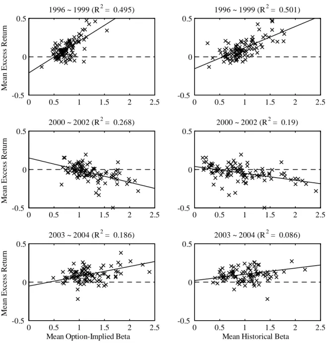
(20) 4.4. The Cross-Section of Returns. Perhaps the most important implications of factor models are cross-sectional. We therefore investigate the cross-sectional performance of the option-implied betas, even though our sample of one hundred …rms observed over nine years is far from ideal to study the cross-section. We regress average 180-day excess returns on average beta in the spirit of Black, Jensen and Scholes (1972). Table 3 presents the results. In Panel A we report the cross-sectional regressions year-by-year. We show results for three di¤erent beta estimates: option-implied beta, historical beta using 180 days of returns, and hybrid beta using option-implied volatilities but correlations from 180 days of returns. We …nd that the model’s cross-sectional performance deteriorates when computing historical and hybrid betas using longer windows. Consider …rst the regressions using historical betas. Note that the slope coe¢ cient is positive for the 1996-1999 years, negative for the 2000-2002 years, and then again positive for the 2003-2004 years. The market movements surrounding the bursting of the dot-com bubble in 2000-2002 are clearly di¢ cult to reconcile with the single-factor model. This pattern is also observed when using option-implied beta. We boldface the R2 for option-implied beta and hybrid beta when it is larger than the R2 from historical beta. Notice that the option-implied beta almost always has a larger R2 than the historical beta. This is not the case for the hybrid beta.12 Panel B reports results for the overall 1996-2004 period. Given the negative slopes on beta during 2000-2002, we also report results for three subperiods. For the overall sample, the slope is positive but small and the …t is better when using historical beta. Figure 7 shows the mean excess return scattered against beta when using option-implied and historical beta respectively. The two beta estimates perform very similarly on the …rst subsample, whereas the option-implied beta performs best on the most recent subsample, perhaps because the options markets are getting more liquid over time. The 2000-2002 period appears as an anomaly with a negative relationship between returns and beta for both beta estimates. It is not straightforward to relate our results to the available literature for a number of reasons. First, we use a short sample because of the limited availability of option data. Second, we use individual stock returns rather than portfolios.13 Third, we use 180-day returns while most of the literature uses monthly returns. Fourth, we investigate a relatively small cross-sectional sample. Fifth, our sample is limited to large cap stocks and therefore the cross-sectional application has limited power to test a given model. For the purpose of this study, we merely conclude that the option-implied beta has signi…cant explanatory power in the cross-section. This is quite remarkable given that the option-implied betas are estimated using only one day of option data. 12 13. We recognize that having a high R2 when the slope estimate is negative is not necessarily desirable. It is well-known that assessing the performance of the CAPM using individual stocks is subject to testing problems. related to measurement error in the betas. See Black, Jensen and Scholes (1972) for an early discussion of this problem. We limit ourselves to one hundred stocks because we want to use liquid option contracts.. 18.

(21) 4.5. Anticipating Ex-Post Realized Beta. We started the empirical investigation in Section 2.3 by assessing the ability of option-implied moments to track changes in future beta. We then derived a new beta estimator using the optionimplied moments. In this section we close the loop and assess the ability of option-implied beta to anticipate changes in future beta. Consider Table 4. We run multivariate regressions of ex-post beta on historical beta and either option-implied or hybrid beta, for each …rm in the S&P100.14 We report for each industry the proportion of stocks where the estimated coe¢ cient for OI or HY BR respectively is statistically signi…cantly estimated. OI refers to option-implied beta and HY BR refers to using option-implied volatilities but historical return correlations. Panel A reports results when the 180-day historical beta is used as the benchmark. Panels B and C repeat the exercise using the 1-year and 5-year historical betas respectively as a benchmark. In each panel, we report on three di¤erent forecasting horizons: 180 days, 1 year and 2 years. This is inspired by the somewhat surprising empirical results discussed in the context of Table 2. While the performance of the option-implied moments for 180-day ex-post betas in Table 2 is impressive, the performance improves even more when using one-year and two-year ex-post betas. First consider Panel A. Of the 100 stocks we investigate, 32% have statistically signi…cant loadings on the option-implied beta at the 180-day forecast horizon, even though the historical beta is included in the regression. When the horizon of interest increases from 180 days to 365 days and 730 days, this percentage improves to 38% and 56% respectively. Panel A also reports results for hybrid beta, where the correlation used for computing the hybrid beta is computed using either 180 days, 1 year or 5 years of daily returns. Clearly the hybrid beta performs well. When forecasting 180-day ex-post betas, the percentage of signi…cant estimates is 32% when computing correlation using 180 days of data. The percentages are 26% and 39% when correlations are computed using 1-year and 5-year windows respectively. The performance of the option-implied as well as hybrid betas improves when forecasting oneyear and two-year ex-post betas. These results are consistent with the results for forecasting using return moments reported in Table 2, and they are somewhat surprising. One potential explanation is the potential problems with ex-post betas evident from Figure 6. As discussed before, ex-post betas often take on implausible values when constructed using a short horizon. This is less often the case when using longer horizons, and this may explain the improved forecasting performance of the option-implied betas. Panels B and C use 1-year and 5-year historical betas respectively as a benchmark, instead of 180-day historical betas as in Panel A. The historical betas computed using longer windows have 14. When implementing forecasting regressions, one potential problem is overlapping data (see Christensen and Prab-. hala (1998)). Two potential solutions are to use instrumental variable techniques and to use non-overlapping data. Instrumental variable regressions were noninformative because of the poor quality of the instruments. Regression results were very similar when using a sample of non-overlapping data based on 30-day betas.. 19.

(22) less forecasting power, as is evident from Figure 6, and as a result the option-implied and hybrid betas perform relatively better overall. The improvements provided by option-implied and hybrid betas di¤er across sectors. For the industrials, consumer discretionary, materials, and IT sectors, they perform well. Their performance is generally weaker for the consumer staples and health care industries. In Table 5, we cross-sectionally regress the improvement in correlation o¤ered by option-implied and hybrid betas on various …rm characteristics. We only report results obtained using the 180-day historical return as the benchmark, as this is the best performing historical beta. Each regressor is normalized by dividing by its standard deviation. Note that for all horizons and for both optionimplied and hybrid beta the distance of average ex-post beta from one is negative and signi…cant. Thus option-implied betas have relative di¢ culty when the ex-post beta is far from unity. This e¤ect is particularly strong for option-implied beta and was evident already in Figure 4 where on average the option-implied beta tended to be closer to one than ex-post beta. Note again that the approach commonly used for historical betas which shrinks the betas toward unity may lessen this e¤ect. The mean ex-post beta variable is signi…cant in two of three option-implied beta cases, suggesting that option-implied beta performs better for higher-beta stocks. Firm size is signi…cantly negative in two of three option-implied columns, indicating that option-implied beta performs better for the smaller …rms in the sample. Recall however that all the …rms we consider are large caps. The option volume is positive in two of the three option-implied columns. This may suggest that estimates of the option-implied moments will improve as option markets become more liquid. We therefore expect that as option market liquidity continues to improve, the added value of using option-implied information to compute beta will increase.. 4.6. Combining the Information in Historical and Option-Implied Beta. So far we have focused on comparing betas computed from option prices with those computed from returns. In this section we instead ask if there is scope for combining the two types of beta. They are computed using very di¤erent information sets and so it is likely that the option-based betas complement the information in traditional return-based betas. In order to assess the potential bene…ts of combining betas we investigate multivariate regressions of ex-post realized beta on the two kinds of betas. The multivariate forecasting regression is REAL t;t+H. where OI t. REAL t. =. is ex-post realized beta,. 1. +. OI 2 t. HIST t. +. HIST 3 t. + ut;t+H. (13). is the (best-performing) 180-day historical beta, and. is the option-implied beta computed using option prices on day t only.. The results using a horizon H of 180, 365, and 730 days are reported in Table 6. We run pooled panel regressions of the ex-post beta on the forecasted betas, either by industry or by size decile. For the industry-based results in Panel A, the coe¢ cient on historical beta is positive and signi…cant 20.

(23) virtually everywhere. When using a horizon of 180 days for ex-post beta, the option-implied beta coe¢ cient is positive and signi…cant in …ve cases. Point estimates are large but usually smaller than the loadings on the historical betas, indicating that the information in the historical beta is more important. Looking next at the 365-day horizon, the option-implied beta is positive and signi…cant in six cases. The results for the 730-day horizon are similar: seven signi…cant option-implied betas. The results across industries largely con…rm the …ndings from Table 4: the option-implied betas perform best for the materials, industrials, and consumer discretionary sectors. These results suggest that the option-implied beta is complementary to the information in historical beta for predicting future beta. Once again, we obtain the interesting result that options contain important information for forecasting ex-post betas computed over horizons that exceed the options’maturities. In Panel B, both the historical beta and the option-implied betas are positive and signi…cant in virtually every case. Unlike the case of the industry results, few patterns emerge as a function of …rm size. In summary, option-implied betas complement historical betas. Option-implied betas are computed using a very di¤erent information set than the one used for historical betas. This makes them useful in combination with the historical beta. We emphasize again that the option-implied beta is computed using only one day of data, and its performance is therefore quite remarkable.. 5. Concluding Remarks. Market betas are one of the most important concepts in the practice and theory of …nance, and for many interesting applications of market betas, such as computing the cost of capital, out-ofsample performance is key. Currently, market betas are obtained by using regression techniques on historical data. Many historical implementations use a simple rolling regression approach, while other approaches allow more explicitly for time-varying betas.. However, no matter how. sophisticated the approach, historical betas implicitly assume that the past o¤ers a good guide to the future. This paper presents a radically di¤erent approach that extracts betas from option data. Because option data contain information about the future, this approach is inherently forward-looking. The approach is inspired by the literature on volatility forecasting, where a number of authors have compared the forecasting performance of implied volatility with that of more traditional historical methods. The strength of our approach is that betas can be computed using a single cross-section of option data, which may be an important advantage when a company experiences (potential) changes in its operating environment or capital structure. We test our method using a very conservative approach, by investigating how it compares with historical methods on average, including stable periods. We …nd that the option-implied estimates perform relatively well. Option-implied betas that were extracted for equities with liquid options. 21.

(24) often outperform the historical market beta in predicting the future beta in the following period. In some cases, combining historical betas with option-implied betas further improves results. We also provide a detailed study of the hybrid beta method proposed by French et al. (1983). Hybrid betas that combine option-implied volatilities with historical correlations perform very well. Optionimplied and hybrid betas also explain a sizeable amount of the cross-sectional variation in expected returns. Much remains to be done. The computation of the option-implied beta uses moments extracted from options data. While we have made full use of recent innovations in the implementation of these procedures, and added some innovations ourselves, it may be that the out-of-sample performance of the option-implied betas can be improved through more e¢ cient estimation of moments. Alternatively, it may be possible to better estimate option-implied correlation using the methods of Carr and Madan (2000). Also, we have not provided an explanation for the relatively poor performance of option-implied betas for stocks with very small ex-post betas, and the di¤erences in performance across industries also merit further investigation. Another remaining question is if option-implied beta performs even better in situations and time periods that can a priori be labeled as inherently unstable. It may also prove interesting to investigate the optimal combination of option-implied and historical betas, which is of course related to the previous question. Finally, we note that it may be possible to compute option-implied betas that are estimated for a particular purpose using the relevant statistical loss function, for instance in a portfolio model (Granger (1969)). Our technique can be used for a variety of applications, such as the detection of abnormal returns in event studies, and the uncovering of abnormal returns for portfolio management. The very de…nition of the word “event”indicates that some aspects of the …rm or the …rm’s environment change, and therefore it will prove interesting to contrast the results obtained using option-implied betas with those obtained using historical betas. One particularly promising application is the computation of the cost of capital for newly merged companies. The main focus in this paper has been on forecasting 180-day ex-post betas, which are relevant for certain applications such as abnormal returns. For other applications, such as cost of capital calculations, longer-horizon betas may be needed. We plan to investigate the performance of optionimplied betas in this context by using LEAPS as well as option contracts with longer maturities traded on non-U.S markets. Indeed, our option-implied beta approach allows for the computation of a complete term structure of beta for each company so long as the options data is available. We compute option-implied moments and betas using option prices on a given day. While this is the most obvious and transparent initial approach to investigating the method’s merits, the performance of the option-implied betas may be improved by adjusting these betas using a predetermined rule, or by smoothing betas and/or moments using information extracted from option prices on other days. The optimal use and optimal smoothing of information contained in option prices is certainly worthy of further study. Finally, we have compared and combined the option-implied betas with simple historical betas. 22.

(25) from daily data. Option-implied betas could alternatively be compared and combined with other methods. Many alternatives exist, including realized betas from intraday data as in Andersen et al (2006), the GARCH betas in Bollerslev, Engle, and Wooldridge (1988), the stochastic Bayesian beta in Jostova and Philipov (2005), simple Bayesian adjustments to OLS such as Vasicek (1973), or commercial beta estimates such as those from BARRA, Bloomberg and Ibbotson.. 6. Appendix A: Replicating Payo¤ Functions. Carr and Madan (2001) show that any twice continuously di¤erentiable payo¤ function f (S) can be replicated with bonds, the underlying stock and the cross section of out-of-the-money options. For convenience, we replicate their argument here. The fundamental theorem of calculus implies that for any …xed F. f (S) = f (F ) + 1S>F. = f (F ) + 1S>F. ZS. F ZS F. 0. f (u)du. 1S<F. ZF. f 0 (u)du. S. 2. 4f 0 (F ) +. Zu. F. 3. f 00 (v)dv 5 du. 1S<F. ZF S. 2. 4f 0 (F ) +. Because f 0 (F ) is not a function of u we are able to apply Fubini’s theorem 0. f (S) = f (F ) + f (F )(S. F ) + 1S>F. ZS ZS. 00. f (v)dudv + 1S<F. F v. ZF Zv. ZF u. 3. f 00 (v)dv 5 du. f 00 (v)dudv. S S. Now integrate over u 0. f (S) = f (F ) + f (F )(S. F ) + 1S>F. ZS. 00. f (v)(S. v)dv + 1S<F. F. = f (F ) + f 0 (F )(S. F) +. Z1. f 00 (v)(S. ZF. f 00 (v)(v. S)dv. S. v)+ dv +. ZF. f 00 (v)(v. S)+ dv. 0. F. If we set F equal to the initial stock price, F = S0 ; and integrate over K instead of v, where K is interpreted as the strike, we are left with the spanning equation. f (S) = [f (S0 ). Z1 f (S0 )S0 ] + f (S0 )S + f 00 (K)(S 0. 0. S0. ZS0 K) dK + f 00 (K)(K +. S)+ dK. 0. From this equation we see that the payo¤ f (S) is spanned by a [f (S0 ) f 0 (S0 )S0 ] position in bonds, f 0 (S0 ) position in shares of the stock and a f 00 (K)dK position in out-of-the-money options.. 23.

(26) 7. Appendix B: The Accuracy of the Moment Computations. As we do not have a continuum of option prices available to compute the moments, it is inevitable that certain biases will be induced in the estimation. We conducted a number of Monte Carlo experiments to determine the importance of these biases on the estimation of volatility and skewness, and we used the results of these Monte-Carlo experiments to guide our empirical implementation. There are three types of biases that are of particular concern in the estimation of volatility and skewness: discretization of strike prices, truncation of the integration domain, and asymmetry of the integration domain. Jiang and Tian (2005) examine the e¤ects of discretization and truncation on the computation of option-implied volatility. We closely follow their setup and extend their analysis to the computation of option-implied skewness. To examine the size of the approximation errors induced by these biases, we generate option prices using Heston’s (1993) stochastic volatility model (HSV) with standard parameterization based on the empirical results of Bakshi, Cao and Chen (1997): = V =. 0:5.. = 0:04,. = 2,. v. = 0:225 and. We set the initial instantaneous variance (V ) to be equal to the long-run variance. = 0:04, the initial stock price equal to S0 = 100, and the risk-free rate equal to r = 0:05:. Because we are interested in a 180-day beta, we set the time to maturity equal to 180 days, T = 180=365. To measure the variance and the skewness of the distribution implied by the HSV parameterization we use the following approach. To ensure that we do not encounter negative stock prices or negative variances we use Ito’s Lemma to convert the risk-neutral stochastic volatility dynamics in HSV to d ln S and d ln V . Once we discretize the equations we get the following risk neutral dynamics 1 Vt 2. ln(St+ t ) = ln(St ) + r. ln(Vt+ t ) = ln(Vt ) +. 1 Vt. ( + ). "Vt+ where. t. V. +. = "St+. t. t+. +. p. 1. p p Vt t"St+. 1 2 2". 2 V. (14). t. 1 p t+ p t"Vt+ Vt. t. t+ t. t = 1=252 (assuming that there are 124 trading days in 180 calendar days). By iterating. through these equations 124 times, we can generate a 180-day stock price path. We repeat this ST S0. exercise 250; 000 times, calculate the log returns ln is equal to 0:2037, and skewness, which is equal to. of each path and compute volatility, which. 0:4610: To verify the accuracy of this simulation-. based approach, we compare the call price with strike K = 100 obtained using simulation, CSIM , with the closed form solution CHEST . We …nd CHEST = 6:5905 and CSIM = 6:5780. We now have benchmarks to evaluate the accuracy of our estimation procedure. The …rst bias we investigate results from the discreteness of the strike prices.. To compute the moments. arbitrarily precisely, we need a continuum of option prices from 0 to plus in…nity, while in reality we only have prices at …xed strike price levels.. In the …rst part of this experiment we generate. 24.