DOI:10.1051/agro/2010007
Review article
Modelling soil carbon and nitrogen cycles during land use change.
A review
J. B
atlle
-A
guilar
1*
, A. B
rovelli
1, A. P
orporato
1,2, D.A. B
arry
11Institute for Environmental Engineering, École Polytechnique Fédérale de Lausanne, Station 2, 1015, Lausanne, Switzerland 2Permanent address: Civil and Environmental Engineering Department, Duke University, Durham, NC 27708, USA
(Accepted 9 February 2010)
Abstract – Forested soils are being increasingly transformed to agricultural fields in response to growing demands for food crop. This mod-ification of the land use is known to result in deterioration of soil properties, in particular its fertility. To reduce the impact of the human activities and mitigate their effects on the soil, it is important to understand the factors responsible for the modification of soil properties. In this paper we reviewed the principal processes affecting soil quality during land use changes, focusing in particular on the effect of soil mois-ture dynamics on soil carbon (C) and nitrogen (N) cycles. Both physical and biological processes, including degradation of litter and humus, and soil moisture evolution at the diurnal and seasonal time scales were considered, highlighting the impact of hydroclimatic variability on nutrient turnover along with the consequences of land use changes from forest to agricultural soil and vice-versa. In order to identify to what extent different models are suitable for long-term predictions of soil turnover, and to understand whether some simulators are more suited to specific environmental conditions or ecosystems, we enumerated the principal features of the most popular existing models dealing with C and N turnover. Among these models, we considered in detail a mechanistic compartment-based model. To show the capabilities of the model and to demonstrate how it can be used as a predictive tool to forecast the effects of land use changes on C and N dynamics, four different scenarios were studied, intertwining two different climate conditions (with and without seasonality) with two contrasting soils having physical properties that are representative of forest and agricultural soils. The model incorporates synthetic time series of stochastic precipitation, and therefore soil moisture evolution through time. Our main findings in simulating these scenarios are that (1) forest soils have higher concentrations of C and N than agricultural soils as a result of higher litter decomposition; (2) high frequency changes in water saturations under seasonal climate scenarios are commensurate with C and N concentrations in agricultural soils; and (3) due to their different physical properties, forest soils attenuate the seasonal climate-induced frequency changes in water saturation, with accompanying changes in C and N concentrations. The model was shown to be capable of simulating the long term effects of modified physical properties of agricultural soils, being thus a promising tool to predict future consequences of practices affecting sustainable agriculture, such as tillage (leading to erosion), ploughing, harvesting, irrigation and fertilization, leading to C and N turnover changes and in consequence, in terms of agriculture production.
soil organic matter/ biogeochemical cycles / agricultural soil / forest soil / soil nutrients / soil moisture dynamics / soil restoration
Contents
1 Introduction. . . 2
1.1 Land use change: forest versus agricultural soils. . . 2
1.2 Modelling of soil C and N cycles. . . 3
2 C and N cycles in soil. . . 3
3 Moisture dynamics as a controlling factor of soil carbon and nitrogen cycles. . . 5
4 Existing models of soil carbon and nitrogen turnover. . . 6
5 Description of the C-N model . . . 8
6 Modelling scenarios . . . 11
6.1 Climate scenarios . . . 11
6.2 Soil scenarios. . . 12
7 Results. . . 14
8 Conclusions. . . 19
* Corresponding author: [email protected]
1. INTRODUCTION
Soils are complex systems sustaining life on Earth. Among other functions, soils maintain plant and animal growth, recy-cle nutrients and organic wastes, filter and purify water. Pre-cisely, soil quality refers to a combination of chemical, physi-cal, and biological processes that confers to the soil the ability to carry out, among others, these particular ecological func-tions. Numerous human activities however utilise soil, mod-ify its physical and chemical properties and change the com-position of its ecosystems. As a result, in the last century a widespread decrease of soil quality has been observed, to-gether with a deterioration of its functioning (Brady and Weil, 2004).
The main component of soils is organic matter (SOM), which shows a variable degree of decomposition, from fresh litter to highly decomposed humus. SOM stores three to four times the amount of carbon (C) than found in all liv-ing vegetation. Other than C, soils also contain nearly all the macro- (nitrogen, N, phosphorous, P, and potassium, K) and micro-nutrients required by living organisms. Among the macronutrients N plays a major role since it is essential for life but its bio-available forms are seldom abundant in the environ-ment. Therefore in many ecosystems the N cycle controls the overall soil turnover and functioning. For these reasons and without neglecting the importance of other nutrients, in this paper the focus is on soil C and N cycles.
1.1. Land use change: forest versus agricultural soils
The increasing demand on food crops, pasture, firewood and timber is at the origin of worldwide changes of land-use in forested areas. This situation is worrying in some ar-eas of the planet, such as South America, where 12% and 7% of forestland was converted to pasture and croplands, respec-tively, between 1850 and 1985 (Houghton et al.,1991). Land-use changes, and especially cultivation of previously forested land, reduce significantly the soil quality (e.g., changes in SOM content and decomposition rates, changes in soil chem-ical and physchem-ical properties), leading to a permanent degra-dation of land productivity (Nye and Greenland,1964; Islam et al.,1999). Furthermore, it has been reported that deforesta-tion increases carbon dioxide (CO2) release to the atmosphere
(Houghton,2002), which contributes to global warming. All studies that focused on the effects of land conversion from forest to cultivated land concluded that land-use change induces a reduction of the available soil C and a decrease in its quality. The maximum rate of loss occurs during the first 10 y of cultivation, with total C decrease up to 30% (Davidson and Ackerman,1993; Lugo and Brown,1993; Murty et al.,2002) followed by reduced but still significant reduction rate (Brams, 1971; Martins et al.,1991; Bonde et al.,1992; Motavalli et al., 2000). Furthermore, it was reported that the loss rate is highly variable and influenced by several factors such as the na-tive vegetation, climate, soil type and management practices (Mann,1986; Davidson and Ackerman, 1993; Bruce et al., 1999).
Contrasting with the conversion from forest to cultivated land, controversy exists when the change is from forest to pas-ture lands. The overall change in soil C has been shown to be either positive or negative. For instance, de Moraes et al. (1996) found an increase up to 20% in total soil C 20 y after the change in land use, while Veldkamp (1994) reported a net soil organic C loss up to 18% after 25 y. Johnson (1992) also observed that changes in soil C in both land-use cultivation and pasture were associated with changes in soil N. Reiners et al. (1994) found that the transformation of forest land to pas-ture led to important changes in the N cycling. For example, the ammonium (NH+4) pool was larger in pasture lands while the nitrate (NO−3) pool was less important in pasture than for-est lands. This is consistent with a low rate of plant uptake of NH+4 and slow nitrification rates (Vitousek,1984; Vitousek and Sanford,1986).
One of the important aspects that affect SOM cycling in the transition from forest to cultivated soil is the removal of most of the fresh organic C (litter) due to harvesting (Smil, 1999). However, harvesting is not the only factor responsible for the soil organic C loss. Some other processes that were also recognized to contribute to change the amount of soil C are the changes in litter chemical properties (Feigl et al., 1995; Ellert and Gregorich,1996; Scholes et al.,1997), soil type (Feller and Beare, 1997; Scholes et al., 1997; García-Oliva et al.,1999), microbial community (Prasad et al.,1995), changes in soil N cycling (Dalal and Mayeer,1986; Brown and Lugo,1990; Desjardins et al.,1994) and management prac-tices (Feller and Beare, 1997; Fernandes et al.,1997; Bruce et al., 1999). Soil tillage and ploughing promote redistribu-tion of residues and their decomposiredistribu-tion. As a result, soil C and N pools are depleted and soil fertility is lost. Soil C is oxidized to CO2 and lost to the atmosphere contributing to
the increase of greenhouse gases in the atmosphere. Moreover, tillage improves soil aeration, destroys macro-aggregates and changes the hydrological cycle, with an increase of the res-piration rates and ultimately an additional depletion of the C pool (Juo and Lal,1979; Agboola,1981; Ellert and Gregorich, 1996; Reicosky et al.,1997; Bruce et al.,1999).
In agricultural areas, the root zone (soil depth affected by plant roots) remains constant over time and is relatively shal-low. Different rooting patterns have direct effects on the C flux, since they affect soil porosity and soil aeration (Berger et al., 2002). Therefore, changes in land use resulting in a modified rooting depth often have a direct influence on soil respiration and C mineralization rates, and thus on soil turnover (Howard and Howard,1993).
Ecological restoration is the process of assisting the recov-ery of an ecosystem that has been degraded, damaged or de-stroyed as a consequence of human activities (Young et al., 2005), and typically involves a land use change. During the restoration, environmental conditions (e.g., type of vegetation, ecosystem corridors or soil practices) are manipulated to cre-ate ecological conditions suitable for the successful establish-ment of a target composition of species (Prober et al.,2005). The change from agricultural soil to the original forest is a typical example of soil restoration, where natural soil proper-ties and vegetation are amended, resulting in an improvement
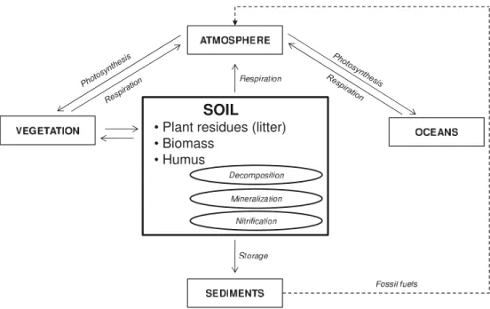
Figure 1. Simplified representation of the global carbon cycle.
of soil fertility and an ecosystem close to its former natural condition.
1.2. Modelling of soil C and N cycles
Numerical tools are becoming increasingly used to under-stand the modifications induced in ecosystems as a result of changes in land use, and it has been found that understanding the coupled N and C dynamics is of primary importance for predictive models of SOM evolution, for example to changes in land use and responses to global changes (Rodriguez-Iturbe et al.,2001). Modelling of soil biogeochemical processes dates back to the 1930s (Manzoni and Porporato,2009), and nowa-days an extended list of stochastic, empirical and mechanistic models incorporating soil nutrient dynamics is available. Mod-els vary significantly in terms of complexity and mathematical description of the biological and geochemical processes in-volved. Manzoni and Porporato (2009) reviewed and classified about 250 different mathematical models developed over 80 y. Most of the models currently available evolved from early ef-forts to provide a concise mathematical description of the soil cycles, and have been adapted and improved to specific appli-cations. The aims of the different models are numerous and include, for example: understanding and prediction of feed-backs between terrestrial ecosystems and global climate (e.g., estimate and predict climatological and biological effects of human activities) (Agren et al.,1991; Melillo,1996; Moore et al.,2005); influence of climate changes on nutrient cycling in soils (Pastor and Post,1986; Hunt et al.,1991; Moorhead et al., 1999; Eckersten et al.,2001; Ito,2007); prediction of changes in soil C and N cycles related to possible land use changes (Eckersten and Beier,1998; Paul and Polglase,2004; Christiansen et al.,2006; Findeling et al.,2007; Pansu et al.,
2007; Post et al.,2007; Kaonga and Coleman,2008); and fore-casts of crop productivity and system response under specific physical soil changes (Wolf et al.,1989; Wolf and Van Keulen, 1989; Matus and Rodríguez,1994; Parton and Rassmussen, 1994; Henriksen and Breland,1999; Nicolardot et al.,2001).
The aim of this manuscript is to provide an overview of the main processes, mechanisms and parameters affecting the evolution of selected soil nutrient cycles (soil C and N) and to provide a modelling framework that incorporates the key mechanisms. Both physical and biological processes, includ-ing degradation of litter and humus, and soil moisture evo-lution on diurnal and seasonal time scales are considered. In the first part of the manuscript, soil C and N cycles are sum-marized, followed by an overview of the most popular mod-els dealing with soil nutrient turnover. In the second part, a compartment model based on Porporato et al. (2003) is de-scribed and applied to simulate soil C and N dynamics, as well as degradation and transformation processes occurring under different precipitation and soil scenarios. Contrasting soil types and precipitation regimes are considered, to illus-trate modelling capabilities and to show how numerical tools can be used to understand effects of land use changes over soil C and N fluxes and, thus, the feasibility and viability of ecological restoration regarding the modelled ecosystem and surroundings.
2. C AND N CYCLES IN SOIL
The global C cycle can be depicted as consisting of a se-ries of interconnected compartments (terrestrial, aquatic and atmospheric) where C is stored and transformed. Soils are part of the terrestrial C pool (Fig.1). The amount of C stored in the (living and dead) organic matter in soils is three to four
times higher than that in the atmosphere (Bruce et al.,1999). The circulation rates are also high. For these reasons, soil C turnover is of primary importance to developing understand-ing and forecastunderstand-ing global changes in biogeochemical cycles and climate change (Stevenson and Cole,1999; Rodriguez-Iturbe and Porporato,2004). The total global emission of CO2
from soils is probably the largest flux in the global C cy-cle, and small changes in the magnitude of soil respiration, if they take place at large scale, could have a tremendous effect on the concentration of CO2 in the atmosphere (Schlesinger
and Andrews,2000; Murty et al., 2002). By the same argu-ment, soils have also a great potential for long-term C storage. Whether a soil will act as a sink or source of CO2depends on a
number of environmental factors, including climatic variabil-ity and anthropogenic changes in land use, which for example may result in a modified composition of the vegetation and therefore of the quality and quantity of litter inputs (Gignoux et al.,2001).
The principal C exchange processes between soil and at-mosphere are photosynthesis and respiration. Photosynthetic C fixation by plants – often named primary producers – con-verts atmospheric CO2 and is the main source of soil organic
C. Briefly, during photosynthesis CO2 is used as a C source
to produce complex organic molecules, using sunlight as an energy source (e.g., Killham and Foster,1994):
CO2+ H2O+ Energy → CH2O+ O2. (1)
The complex organic molecules produced by plants enter the soil C cycle as decaying organic matter (litter) and are progres-sively converted to simpler molecules. A significant fraction of the organic C introduced in the soil is directly used as an en-ergy source to sustain pedofauna metabolism, and is released again to the atmosphere in form of CO2through respiration:
CH2O+ O2→ CO2+ H2O+ Energy. (2)
Another part of the soil C is assimilated by vegetation and fi-nally transferred to the soil as plant litter, becoming part of SOM (Porporato et al.,2003). Organic C is available in soils in a large variety of forms. Killham and Foster (1994) partitioned the soil organic C into three main pools: insoluble, soluble and biomass. Insoluble soil organic C includes plant residues and partially decomposed material, which forms the litter and the humus. Soluble C is a fraction of the humus further decom-posed and is rapidly assimilated as a substrate by the pedo-fauna. The fast consumption of soluble C explains its often low concentration in the soil (1%) in comparison to insoluble organic C (90%). Soil biomass (9%) consists of microbes and animals (e.g., macroinvertebrates), the decomposition activity of which is mostly responsible for the C decomposition and recycling (Killham and Foster,1994).
Within the soil, organic C is transferred between the dif-ferent pools (or compartments) by means of decomposition processes, which are regulated by environmental conditions (e.g., soil moisture) and the C/N ratio (Brady and Weil,2004). These factors will be discussed subsequently. Litter under-going decomposition is mainly composed of plant residues (fallen leaves, roots, etc.). Decomposition rates are highly vari-able in time, and are mainly controlled by the environmental
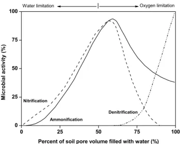
Figure 2. Influence of the soil water content on bacterial activity in different processes of nitrogen transformations (after Fenchel et al., 1998).
conditions (e.g., soil moisture level, aeration, soil temperature) and the quality of the added litter. Complex organic molecules can be decomposed under either aerobic or anaerobic condi-tions. Under normal conditions, soils are unsaturated and thus O2 is likely to be always available. However, even in the
va-dose zone saturated conditions can result from, for example, significant precipitation events. Wetlands are a particular case where saturated conditions are found permanently or season-ally. In general, microbial decomposition rates are larger under aerobic conditions (Brady and Weil,2004), where O2 acts as
the electron acceptor during oxidation of organic compounds (Barry et al.,2002). On the other hand, slow decomposition rates under anaerobic conditions can result in accumulation of considerable amounts of partially decomposed organic matter (Fig.2).
Soil N comes mainly from the atmosphere, which is the largest N pool and contains almost 75% of the total N avail-able on Earth (Barbour et al.,1999). In brief, the soil N cycle is based upon the uptake of the inorganic forms (NO−3, NH+4) by plants. N returns to the soil in organic form as plant residues, which are decomposed by the soil pedofauna (e.g., inverte-brates, microbes, fungi) and are made available to plants in inorganic form.
The total amount of organic N in soils varies greatly and is influenced by the soil-forming factors likely climate, to-pography, vegetation, parent material and age. The N cycle is tightly coupled to the C cycle, since most of the microbial N transformations (e.g., nitrification) use energy supplied by C (Paul,1976). Although locally N is also incorporated into soils through dry or wet direct deposition, the largest fraction of soil organic N fixation is done biologically (conversion from N2
gas to organic forms, mediated by specific microbial strains). N is found in soils mainly within the organic matter fraction, for example humic compounds, plant roots, microbial biomass and decomposing organic materials. The amount of organic N
contained in soils far exceeds that which is present in plant-available inorganic forms.
The soil N, mainly present in organic form as previously mentioned, is almost unavailable for plants. The vegetation mainly uses inorganic forms of N, which are made available by the SOM decomposition. Soil microorganisms convert the N contained in the organic matter to NH+4 in a process named
mineralization (Schinner et al.,1995), further subdivided into two processes. The organic N is initially transformed via
am-monification, and – if O2 is available – NH+4 is subsequently
oxidized to nitrite (NO−2) and NO−3, through nitrification: NH+4+ O2+ H++ 2e−→ NH2OH+ H2O
→ NO−
2 + 5H++ 4e−, (3)
NO−2 + H2O→ NO−3 + 2H++ 2e−. (4)
Although plants can use both forms of inorganic N, NO−3 is used in preference to NH+4 because of its greater solubility in water. In other words, nitrates quickly dissolve in the pore so-lution, which is taken up by plants. On the other hand, how-ever, this also means that NO−3 is easily flushed to groundwater. NH+4 is instead less mobile because it is strongly adsorbed on clay minerals due to its positive charge.
Denitrification is the anaerobic microbial reduction of N,
and NO−3 is used as an electron acceptor (i.e., source of en-ergy), resulting in a transfer of soil N to the atmosphere (Groffman et al.,2002):
2NO−3+ 10e−+ 12H+→ N2(g)+ 6H2O. (5) Immobilisation is a process involving microbial uptake of
nu-trients, where inorganic N is converted into organic form, such as amino acids and biological macro-molecules.
The carbon-to-nitrogen ratio (C/N) is an important factor affecting the overall turnover rates of SOM (Young and Young, 2001). Bacterial sensitivity to the C/N ratio is due to the fact that bacteria need a constant C/N ratio, while this ratio is highly variable in substrate. For example, intense competi-tion among microorganisms for available N occurs when soil residues have a high C/N ratio, i.e., the substrate is poor in N making it the limiting factor (Brady and Weil,2004). Environ-mental conditions (e.g., soil moisture and temperature) have a direct influence on bacterial activity and thus on this ratio (Koch et al.,2007). The C/N ratio of the substrate tends to de-crease as the SOM becomes more decomposed – from fresh litter to highly transformed humus – when microbes are solely responsible for decomposition (Zheng et al.,1999) because the microbial C/N ratio is lower than that of litter (Persson,1983). In other words, the humus is enriched in N compared to the litter. For this reason the C/N ratio of the litter pool controls the rates of mineralization/immobilisation. Young and Young (2001) identified a threshold of the C/N ratio which determines the bacterial activity. When C/N > 25, microbes respire com-pletely using the available C and thus assimilate the entire N mineralized, and consequently N is immobilised. In contrast, if C/N < 25, the SOM N content far exceeds the immobilisation capacity of microbial populations and the result is a net miner-alization. Although this threshold seems to be directly related to the C/N ratio needs of bacteria, White (1997) argued that
this threshold value is variable among different ecosystems, for example because the C/N ratio of the vegetation changes depending on the composition and relative frequency of each species. For example, pines produce litter with C/N ratio as high as 90, while litter originating from cereal crops has C/N ratio of 80 and tropical forest trees produce litter with C/N ratios around 30 (Young and Young,2001).
3. MOISTURE DYNAMICS AS A CONTROLLING FACTOR OF SOIL CARBON AND NITROGEN CYCLES
Soil moisture results from the interactions between climate, soil type (texture, granulometry, organic matter content) and vegetation, and it is consequently variable both in space and time. Among the possible physical processes the dynamics of soil moisture exerts the greatest influence over SOM turnover, mineralization, decomposition, leaching and uptake, and its ef-fects are complex and non-linear. As an example to illustrate this complexity, the production of plant residues – the main source of litter and therefore of energy for the pedofauna – depends on the growth rate of vegetation, which is controlled by water availability. Accumulation of SOM can increase the water retention capacity of the soil, with a positive feed-back on the vegetation. Moreover, the soil biota activity depends on the soil water content, and optimal decomposition rates are only achieved within a relatively narrow soil moisture range.
Soil biota is sensitive to moisture level for several reasons. In order to preserve cell integrity, when the soil water tent decreases bacteria increase the intracellular solute con-centration to compensate for the extracellular concon-centration and counterbalance the increased osmotic pressure (Stark and Firestone,1995; Bell et al.,2008). Therefore, a high concen-tration of solutes results in an inhibition of the enzymatic ac-tivity and therefore decreased cellular acac-tivity. Additionally, as the soil becomes drier, water in soil pores becomes a thin layer covering soil grains and substrate availability becomes diffusion-limited. In consequence, microbial activity is further reduced (Csonka,1989; Stark and Firestone,1995; Fenchel et al.,1998).
It is however difficult to identify a unique threshold mois-ture level under which soil respiration (or microbial activ-ity) diminishes. Davidson et al. (1998) and Rey et al. (2002) estimated that 75% of the soil field capacity corresponds to the soil moisture level below which soil respiration decreases, while according to Xu et al. (2004) a more likely value is 42%. A number of studies have shown that soil moisture effects on soil C and N turnover also depend on the time-scale of in-terest. Curiel Yuste et al. (2007) found that, at the seasonal scale, the effect of temperature and soil moisture on CO2
ef-flux (e.g., soil respiration) was very similar for ponderosa pine and oak savannah ecosystems. For shorter time scales (e.g., daily), decomposition of organic matter was mainly controlled by temperature during wet periods and a combination of tem-perature and soil moisture during dry periods. Soil bacterial growth (or soil respiration) – a parameter often used as a mea-sure of microbial activity – shows a maximum at about 30◦C
(Pietikåinen et al., 2005). Nevertheless, the influence of temperature on microbial activity is generally considered much less important than soil moisture (Rodriguez-Iturbe and Porporato,2004) because, although important differences in soil temperature are likely to occur at a daily and seasonal scale in the uppermost soil (e.g., first few centimetres), yearly average values at depth are much more constant than those of soil moisture.
Typically, summer drought decreases substantially decom-position rates (Curiel Yuste et al.,2007), but it has been ob-served that sporadic rains during these dry periods tends to increase the decomposition efficiency of the bacterial commu-nities (Borken et al.,1999,2002; Savage and Davidson,2001; Goulden et al.,2004; Xu et al., 2004; Misson et al., 2005; Scott-Denton et al.,2006). Kieft et al. (1998) and Moore et al. (2008) observed an increase of root density and soil micro-bial activity rate in response to isolated moisture pulses in arid soils, although the response of root density occurred at longer time-scale. A fast rewetting of the soil profile is likely to have negative consequences on microbial populations in that it can generate an osmotic shock and result in cell lyses (Kieft et al., 1987; Van Gestel et al.,1993). In contrast, Ryel et al. (2004), Schwinning and Sala (2004) and Bell et al. (2008) found that, in arid soils, while plants usually do not take advantage of brief pulses of moisture generated by short precipitation events, microbial mineralization is stimulated. Consequently, short-term increases in soil microbial activity triggered by mois-ture pulses will not typically correlate with an increase in pri-mary production at the same time scale, confirming that plant growth is not only dependent on soil microbial activity, but also on other factors such as the precipitation event duration, amount of soil water infiltrated and the overall change in soil moisture. The magnitude and timing of intra-seasonal precipi-tation becomes therefore a key regulator for microbial activity (Bell et al.,2008). Since decomposition and consequent min-eralization can be stimulated by moisture pulses that are too brief to benefit primary producers (e.g., plants) (Cui and Cald-well, 1997; Schwinning et al., 2003; Austin et al.,2004), in arid soils there is potential for soil nutrient pools to accumulate over time and become available to plants as heavier precipita-tion occurs. The influence of soil moisture over soil nutrient dynamics has been also studied in temperate (Davidson et al., 1998; Buchmann,2000; Reichstein et al.,2003) and tropical forests (Conant et al.,2000; Davidson et al.,2000; Kiese and Butterbach-Bahl,2002; Epron et al.,2004). It was concluded that a strong influence of the soil moisture over microbial ac-tivity exists, but that the degree of correlation varies strongly among different ecosystems (Buchmann,2000; Rustad et al., 2000).
4. EXISTING MODELS OF SOIL CARBON AND NITROGEN TURNOVER
At least 250 models dealing with soil C and nutrient turnover exist (Manzoni and Porporato,2009). Classification of all these simulators is difficult because they are based on a wide range of physical and biogeochemical descriptions of
the processes and the underlying assumptions vary signifi-cantly. Nevertheless, based on their internal structure models describing SOM dynamics can be divided into (1) process-oriented, (multi)-compartment models; (2) organism-oriented (food-web) models; (3) cohort models describing decompo-sition as a continuum; and (4) a combination of model types (1) and (2) (Brussaard,1998; Smith et al.,1998; Post et al., 2007). Process-oriented or compartment models (each com-partment or pool is a fraction of SOM with similar chemi-cal and physichemi-cal characteristics) are built considering the pro-cesses involved in the migration of SOM across the soil profile and its transformations (Smith et al.,1998). Models belonging to this class can potentially have a variable degree of com-plexity, from the simplest case with no compartments (con-sidering degradation as a continuum) to more refined, multi-compartment models, with each multi-compartment composed of organic matter with similar chemical composition or degrad-ability. Process-oriented models can be combined with GIS software, giving a modelling platform well suited for regional-scale studies. Examples of successful coupling between soil turnover and GIS software are CANDY (Franko,1996), CEN-TURY (Schimel et al., 1994) and RothC (Post et al., 1982; Jenkinson et al., 1991). On the other hand, the theoretical compartments that define the structure of multi-compartment process-oriented models are difficult to compare with the mea-surements of SOM fractions, and therefore the testing and val-idation is difficult and limited (Christensen,1996; Elliott et al., 1996). Among the most popular process-oriented models are also DAISY (Hansen et al., 1991), NCSOIL (Molina et al., 1983) and SOILN (Johnsson et al.,1987).
In organism-based models the SOM flows from one organ-ism pool to another, which in turn are classified depending upon their taxonomy or metabolism. The main advantage of organism-oriented models is that the main drivers of SOM fluxes and transformations – the pedofauna – are explicitly ac-counted for. However, as noted in Post et al. (2007), to date there is no general acceptance of the existence of a relation between soil biota abundance and degradation rates. In con-trast, the relationship between degradation rate and amount (or concentration) of substrate, as in process-based models, is well recognized. Simple first-order kinetic rates are often suitable to model the transformations, and the reaction rates can be easily estimated from laboratory experiments and di-rectly used in process-oriented models. Site-specific calibra-tion of organism-oriented models involves the characteriza-tion of the soil microbial consortia and therefore requires more complex techniques, while process-oriented models are less influenced by the features of the microbial communities, and have a larger range of application to different environments. To summarize, process-oriented models are easier to apply and calibrate than organism-oriented, which explains their greater popularity. Nevertheless, organism-oriented models have been proposed by several authors, including Moore et al. (2004), Kuijper et al. (2005), Zelenev et al. (2006) and Cherif and Loreau (2009).
A cohort is a set of items sharing some particular char-acteristic. Cohort models divide SOM into cohorts, which are further divided into different pools (e.g., C, N). Contrary
to process-based models where decay is usually treated as a purely physical or biochemical process, e.g., described by a first-order rate, cohort models consider explicitly microbial physiology as the driving factor of decomposition. An exam-ple of a cohort model was proposed by Furniss et al. (1982), where SOM was divided into three cohorts considering age, origin and size, with each cohort subdivided into a number of chemical constituents. Gignoux et al. (2001) developed SOMCO (soil organic matter cohort), where SOM is divided into different cohorts in a demographic sense, meaning that a cohort is a set of items of the same age. At each time step a new cohort is defined and its fate is followed until its relative amount to total SOM becomes negligible. Other examples of models belonging to this class are those of Pastor and Post (1986), Bosatta and Ågren (1991,1994) and Frolking et al. (2001).
The last group of models consists of a combination of process- and organism-oriented models, which are seldom used because their applicability is limited by the data required to define the organism-oriented components (Smith et al., 1998). Some examples of combined models are proposed by O’Brien (1984) and Paustian et al. (1990).
In order to identify to what extent different models are suitable for long-term predictions of soil turnover, and to understand whether some simulators are more suited to specific environmental conditions or ecosystems, model com-parisons were conducted using long-term experiments and multi-annual datasets. De Willigen (1991) tested 14 differ-ent models comparing their ability to simulate soil N turnover (e.g., mineralization and plant uptake). It was concluded that aboveground processes (e.g., plant growth) were easier to sim-ulate than belowground transformations (e.g., soil water and N content), and that the more complex, multi-compartment models do not necessarily provide better results in terms of predictive capabilities. Rodrigo et al. (1997) compared the ef-fects of soil moisture and temperature variations on nine differ-ent models (NCSOIL; SOILN; DAISY; Kersebaum’s model, Kersebaum and Richter, 1991; MATHILD, Lafolie, 1991; TRITSIM, Mirschel et al.,1991; NLEAP, Shaffer et al.,1991; SUNDIAL, Bradbury et al., 1993; CANTIS, Neel,1996) on predictions of soil C and N turnover. Not surprisingly, they observed the highest C decomposition and N mineralisation rates close to field capacity conditions and decreasing rates during soil drying. In this study good agreement between the different models for low moisture conditions was observed, whereas poor agreement was found in wet soils, with wa-ter saturation equal or above field capacity. A complete com-parison of nine process-oriented multi-compartment models (CANDY; NCSOIL; RothC; DAISY; CENTURY, Parton et al., 1987; Verberne model, Verberne et al.,1990; ITE, Thornley, 1991; DNDC, Li et al.,1994; SOMM, Chertov and Komarov, 1997) was presented by Smith et al. (1997). A qualitative and quantitative evaluation of the performance of the models was carried out by comparing their ability to simulate observed data from seven different sites in temperate regions. A general conclusion of all these comparisons was that the errors derived from the tested models are not significantly different, mean-ing that the models provide consistent results except when a
model is used for an application for which it was not oped. For example, the ITE and SOMM models were devel-oped for grasslands while in the study of Smith et al. (1997) they were applied to crops. Model calibration is an additional source of uncertainties and makes the comparison of differ-ent models difficult. Pansu et al. (2004) presented a qualitative comparison of the predictive performance of a family of five multi-compartment models, MOMOS-2 to -6, using14C- and 15N-labelled species in field experiments. These models use
the same conceptual approach but have different complexity, in that the number of compartments varies from 3 to 5 and the description of the biochemical transformation uses a different level of detail and simplification. Pansu et al. (2004) concluded that the simplifications do not decrease significantly model ac-curacy, but that the use of additional compartments results in improved long-term predictions.
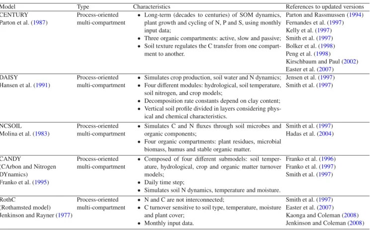
Most of the currently available models are updated versions of earlier and original versions that have been modified to ex-tend the applicability to specific ecosystems. TableIpresents a list of the five most popular models, their main features together with the key references. The popular CENTURY model, originally devised for modelling soil nutrient dynamics in grassland systems, has been considerably modified since its first version. Smith et al. (1997) and Parton and Rassmussen (1994) modified the CENTURY model for application to crop and pasture systems, while Kelly et al. (1997), Peng et al. (1998) and Kirschbaum and Paul (2002) modified the model to be applied to forest ecosystems. Despite the ad hoc modi-fications, contrasting results in terms of predictive capabilities were obtained. The RothC model of Jenkinson et al. (1990), is an evolution of the model previously presented by Jenkinson and Rayner (1977), named Rothamsted. TOUGHREACT-N (Maggi et al.,2008) was developed to study the biogeochemi-cal soil N cycle under different conditions of fertilization and irrigation. It is based on the multi-phase, multi-component re-active transport model TOUGHREACT (Xu et al.,2006), in turn an evolved and improved version of TOUGH2 (Pruess et al.,1999). SWIM (Krysanova et al.,1998), based on pre-viously developed tools (MATSALU, Krysanova et al.,1989; SWAT, Arnold et al.,1993) and originally devised for mod-elling soil N cycle in mesoscale watersheds (102to 104km2),
has recently been extended to better describe groundwater dy-namics and processes in riparian zones (Hattermann et al., 2004; Wattenbach et al., 2005). FullCAM (Richards, 2001) accounts for full C turnover in forests, and is an integrated suite of sub-models: the empirical C tracking model CAM-For (Richards and Evans,2000), the tree growth model 3PG (Landsberg and Waring,1997), the litter decomposition model GENDEC (Moorhead and Reynolds, 1991) and the soil C turnover model RothC (Jenkinson, 1990). PASTIS (Lafolie, 1991; Garnier et al.,2001,2003) is a one-dimensional mecha-nistic model that simulates the transport of water, solutes and heat using Richards’ equation for water flow, the advection-dispersion equation for solute transport and the diffusion equa-tion for heat flow. Some variaequa-tions to this model have been implemented, such as PASTISmulch (Findeling et al., 2007),
which extends the original capabilities by including the physi-cal effects of a surface residue mulch on rain interception and
Table I. Main characteristics of the five most popular models.
Model Type Characteristics References to updated versions
CENTURY Parton et al. (1987)
Process-oriented multi-compartment
• Long-term (decades to centuries) of SOM dynamics, plant growth and cycling of N, P and S, using monthly input data;
• Three organic compartments: active, slow and passive; • Soil texture regulates the C transfer from one
compart-ment to another.
Parton and Rassmussen (1994) Fernandes et al. (1997) Kelly et al. (1997) Smith et al. (1997) Bolker et al. (1998) Peng et al. (1998)
Kirschbaum and Paul (2002) Easter et al. (2007) DAISY
Hansen et al. (1991)
Process-oriented multi-compartment
• Simulates crop production, soil water and N dynamics; • Four different modules: hydrological, soil temperature,
soil nitrogen, and crop models;
• Decomposition rate constants depend on clay content; • Vertical soil profile divided in layers considering
phys-ical and chemphys-ical characteristics.
Jensen et al. (1997) Smith et al. (1997) NCSOIL Molina et al. (1983) Process-oriented multi-compartment
• Simulates C and N fluxes through soil microbes and organic components;
• Four organic compartments: plant residues, microbial biomass, humus and stable organic matter.
Smith et al. (1997) Hadas et al. (2004)
CANDY
(CArbon and Nitrogen DYnamics)
Franko et al. (1995)
Process-oriented multi-compartment
• Composed of four different submodels: soil temper-ature, hydrological, crop and organic matter turnover models;
• Daily time step;
• Simulates soil N dynamics, temperature and moisture.
Franko et al. (1996) Franko et al. (1997) Smith et al. (1997)
RothC
(Rothamsted model) Jenkinson and Rayner (1977)
Process-oriented multi-compartment
• N and C are not interconnected;
• C turnover sensitive to soil type, temperature, moisture and plant cover;
• Monthly input data.
Smith et al. (1997) Easter et al. (2007) Kaonga and Coleman (2008) Jenkinson and Coleman (2008)
evaporation. Another example of model evolution is the family of models MOMOS-2 to -6, which are modified versions from the initial MOMOS-C (Sallih and Pansu,1993) and MOMOS-N (Pansu et al.,1998) models. TRIPLEX (Peng et al.,2002) is a model of forest growth and C and N dynamics, and is a com-bination of three prior well-established models: 3PG (Lands-berg and Waring,1997), TREEDYN3.0 (Bossel, 1996) and CENTURY4.0 (Parton et al.,1993). Easter et al. (2007) de-veloped a soil C modelling system, GEFSOC, aimed at mod-elling soil C stocks and exchange rates at regional or country scales in response to land use changes. The developed tool is based on three well-recognized models: the CENTURY gen-eral ecosystem model, the RothC soil C decomposition model and the empirical IPCC method (IPCC,2003) for assessing soil C stock changes at regional scales. The model can be cou-pled to a soil and terrain digital database to include the topog-raphy and spatial soil variability of the studied area.
5. DESCRIPTION OF THE C-N MODEL
The model we describe and use in this work was pre-sented by Porporato et al. (2003). It belongs to the group of process-based models, with the soil organic matter and nutri-ents divided into five pools. Three pools consist of SOM (litter, humus and microbial biomass), while the remainder are for
in-organic N. The model is applied to the root zone treated as a single unit, i.e., spatial variations are ignored.
The framework with three organic pools is in good agree-ment with Jenkinson (1990), who proposed that process-based models should have between two and four pools to obtain re-liable results. These pools represent the main components of the system, and C and N concentrations correspond to aver-age values over the rooting depth (Zr) (Rodriguez-Iturbe and
Porporato,2004). This simplification is justified because soils have often a uniform distribution of SOM and inorganic N over the whole rooting depth (Porporato et al.,2003). This is not true however for the uppermost soil layer, where organic residues tend to accumulate, and acts as a source of litter to the layers beneath.
Additionally, some other simplifications were made dur-ing the development. First, SOM decomposition rates are known to vary over orders of magnitude among the different components and, as already described, each functional group of organisms has specific and highly variable decomposition and mineralization rates. In the model however no distinc-tion is made between different microbial populadistinc-tions. Rather, for each pool, a single, first-order kinetic rate is used, which represents an average transformation rate. This approach, al-though approximate, reduces the number of model parameters and therefore simplifies its calibration. Decomposition rates vary however among the different pools: litter has faster de-composition than the humus pool. The second approximation
concerns the C/N ratio. As for the transformation rates, the model considers a single C/N ratio for each pool, again rep-resenting an average value. In this case, the litter C/N ratio can be computed, for example, as the weighted average of the C/N ratios of the different species, weighted by their relative amount in the ecosystem. Other than this, vegetation charac-teristics (maximum evapotranspiration, wilting point, incipi-ent stress point, etc.) are assumed constant. This is an impor-tant simplification, since in previous sections it was pointed out that climatic conditions influence vegetation growth and deposition of fresh organic matter. The advantage is that we reduce and simplify the external factors influencing C and N turnover to soil type and moisture content dynamics.
Model inputs are precipitation and litter fall rates, while on output the extent of soil respiration, plant uptake, transpira-tion and leaching are recovered. The amount and frequency of precipitation are the only climatic variables considered. Isothermal conditions are assumed, meaning that variations of the average daily temperature within the year are limited. This assumption is clearly not satisfied in many climatic regions (e.g., at high latitude). On the other hand, the model can still be applicable given that, during the unfavourable season (too high or low temperature), the moisture content becomes an additional limiting factor, thus inhibiting soil respiration and transformations.
The model of Porporato et al. (2003) is comprised of a set of coupled non-linear ordinary differential equations. Each equation describes the mass balance of C and N in the five pools. An overview of the reaction network is given in Fig-ure3. Moreover, since the soil moisture is the key factor in this model, and influences the decomposition and turnover rates as outlined above, soil water variations are computed from the water balance at one point. In order to facilitate model under-standing and comparison with previous works, here we use the same notation as in Porporato et al. (2003), D’Odorico et al. (2004) and Rodriguez-Iturbe and Porporato (2004).
The evolution of C in the litter, humus and biomass pools is given by: dCl dt = ADD + BD − DECl, (6) dCh dt = rhDECl− DECh, (7) dCb dt = (1 − rh− rr)DECl+ (1 − rr)DECh− BD, (8)
where Cl, Chand Cbare the C concentrations in the litter,
hu-mus and biomass pools respectively [M L3], ADD is the
exter-nal input of C to the system [M L−2T−1], BD is the recycling rate of decaying biomass in the litter pool [M L−3T−1], DECl
and DEChare the C fluxes leaving the litter and humus pools
due to microbial decomposition [M L−3T−1], while rhand rr
are non-dimensional coefficients representing the fractions of decomposed organic C that go into the humus pool and to res-piration, respectively.
The combination of equations (6)–(8) gives the overall C balance equation (Ctot) in the system:
dCtot
dt = ADD − rrDECl− rrDECh. (9)
The flux of C between two pools is described by first-order kinetic equations (DECl, DECh and BD), where the reaction
rates (kl, khand kd, respectively) are weighted averages of the
decomposition rates of the different organic molecules. The first-order kinetic equations of C decomposition and microbial death for the litter, humus and biomass pool are:
DECl= φ fd(s) CbklCl, (10) DECh = φ fd(s) CbkhCh, (11)
BD= Cbkd, (12)
whereφ is a non-dimensional factor that accounts for a possi-ble reduction of the decomposition rate when the litter is very poor in N (high C/N ratio) and the immobilization is not suf-ficient to integrate the required N by the bacteria. This factor has an important influence on the dynamics of the biomass evolution, and details on how it is defined and computed can be found in Porporato et al. (2003). The term fd(s) is a
non-dimensional parameter that describes soil moisture effects on decomposition: fd(s)= ⎧⎪⎪ ⎪⎪⎨ ⎪⎪⎪⎪⎩ s sf c, s ≤ s f c, sf c s , s > sf c, (13)
where Sf cis the soil field capacity (water content held in soil
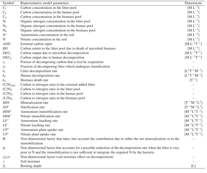
after excess water drained away by gravity). The main model parameters are listed in TableII.
The N balance in the litter, humus and biomass pools is computed from the C balance equations, scaled by the appro-priate C/N ratio: dNl dt = ADD (C/N)add + BD (C/N)b − DECl (C/N)l , (14) dNh dt = rh DECl (C/N)h − DECh (C/N)h, (15) dNb dt = [1 − rh (C/N)l (C/N)h ]DECl (C/N)l + DECh (C/N)h − BD (C/N)b − Φ, (16) where Nl, Nhand Nbare the N concentrations in the litter,
hu-mus and biomass pools, respectively [M L−3T−1], (C/N)add,
(C/N)l, (C/N)h and (C/N)b are the C to N ratios of added
or-ganic matter, litter, humus and biomass pools, respectively, andΦ is a term that takes into account the contribution due to either the net mineralization or to the immobilization [M L−3T−1]. This term relates the total mineralization and immo-bilization rates:
Φ = MIN − IMM, (17)
where MIN expresses the mineralization rate [M L−3T−1] and
IMM is the total rate of immobilization (sum of the N
immo-bilization rate in the NH+4 IMM+ and NO−3 IMM− pools, re-spectively) [M L−3T−1]. When IMM is equal to zero, MIN is
Nitrogen plant uptake
Figure 3. Schematic representation of soil C and N cycles (after Rodriguez-Iturbe and Porporato, 2004).
equal toΦ, while when MIN is zero IMM is equal to –Φ. The (C/N)b ratio is one of the most important parameters in the
model, since the switch between mineralization and immobi-lization is defined in order to maintain as constant the C/N ra-tio of the biomass pool. If the organic matter is rich in N (and (C/N)bis smaller than the value required to sustain growth of
microbial biomass), decomposition results in surplus N. This is used by the microorganisms, and mineralization occurs. In contrast, if decomposition produces an environment poor in N, microorganisms will increase the immobilization rate of NH+4 and NO−3 in order to meet their requirements. This process is rather complex and very dynamic, as explained in Porporato et al. (2003).
N transfer between the pools is described by the same first-order kinetic transfer parameters used for C, with each term scaled by the corresponding C/N ratio (Fig.3). The balance equations of inorganic N are:
dN+ dt = MIN + IMM +− NIT − LE+− UP+, (18) dN− dt = NIT − IMM −− LE−− UP−, (19)
where N+ and N− are the inorganic N concentrations in the NH+4 and NO−3 pools, respectively [M L3], NIT is the
nitri-fication rate [M L−3T−1], UP+and UP−are the N uptake by plants from the NH+4 and NO−3pools, respectively [M L−3T−1], and LE+and LE−are N fluxes from the root zone towards the groundwater [M L−3T−1].
The combination of equations (14–16, 18, 19) gives the overall evolution of total N (Ntot) in the system:
dNtot dt =
ADD
(C/N)add − LE
+− UP+− LE−− UP−. (20)
Equations (9) and (20) represent the total C and N sinks and sources of the system depicted in Figure3.
Although we have described the main elements of the model here, further descriptions – for example the rates of mineralization (MIN), immobilization (IMM+and IMM−), ni-trification (NIT), plant uptake (UP+ and UP−) and leach-ing (LE+ and LE−) and their associated variables – can be found in Porporato et al. (2003), D’Odorico et al. (2004) and Rodriguez-Iturbe and Porporato (2004), together with addi-tional discussion about the underlying assumptions and sim-plifications introduced in this model.
Table II. Summary of the main parameters considered in the soil C-N model.
Symbol Representative model parameters Dimensions
Cl Carbon concentration in the litter pool [M L−3]
Ch Carbon concentration in the humus pool [M L−3]
Cb Carbon concentration in the biomass pool [M L−3]
Nl Organic nitrogen concentration in the litter pool [M L−3]
Nh Organic nitrogen concentration in the humus pool [M L−3]
Nb Organic nitrogen concentration in the biomass pool [M L−3]
N+ Ammonium concentration in the soil [M L−3]
N− Nitrate concentration in the soil [M L−3]
ADD External carbon input [M L−2T−1]
BD Carbon return to the litter pool due to death of microbial biomass [M L−1] DECl Carbon output due to microbial decomposition [M L−3T−1]
DECh Carbon output due to humus decomposition [M L−3T−1]
rr Portion of decomposing carbon that is lost by respiration –
rh Fraction of decomposing litter which undergoes humification –
kl Litter decomposition rate [L3T−1M−1]
kh Humus decomposition rate [L3T−1M−1]
kd Biomass death rate [T−1]
(C/N)add Carbon to nitrogen ratio in the external added litter –
(C/N)l Carbon to nitrogen ratio in the litter pool –
(C/N)h Carbon to nitrogen ratio in the humus pool –
(C/N)b Carbon to nitrogen ratio in the biomass pool –
MIN Mineralization rate [T−1M−1L3]
NIT Nitrification rate [T−1M−1L3]
IMM+ Ammonium immobilization rate [M−1L3T−1]
IMM− Nitrate immobilization rate [M−1L3T−1]
LE+ Ammonium leaching rate [M−1L3T−1]
LE− Nitrate leaching rate [M−1L3T−1]
UP+ Ammonium plant uptake rate [M−1L3T−1]
UP− Nitrate plant uptake rate [M−1L3T−1]
Φ Non-dimensional factor that takes into account the contribution due to either the net mineralization or to the immobilization
– φ Non-dimensional factor that accounts for a possible reduction of the decomposition rate when the litter is very
poor in N and the immobilization is not sufficient to integrate the required N by the bacteria
– fd(s) Non-dimensional factor (soil moisture effect on decomposition) –
s Soil moisture –
Zr Rooting depth [L]
6. MODELLING SCENARIOS
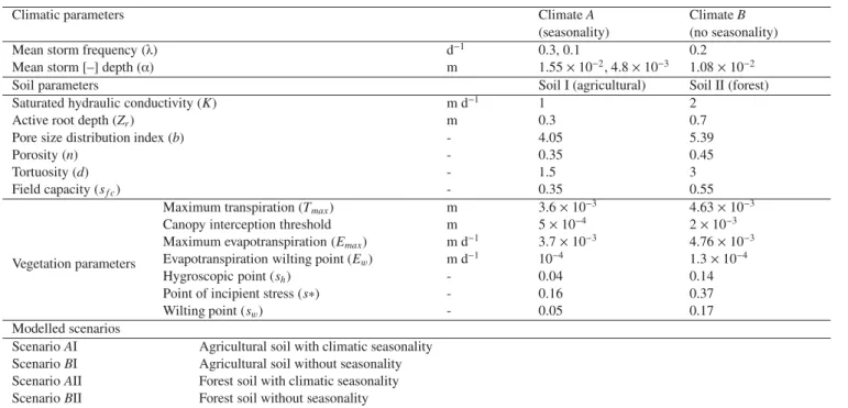
It has been shown in previous sections that land use change and hydroclimatic conditions are the main factors contribut-ing to changes in soil C and N turnover. To test the relevance of mechanisms and parameters contributing to the fate of soil C and N, different modelling scenarios were simulated, for which the main variables are presented in TableIII. The com-bination of two different soils and two different climatic con-ditions gives four different scenarios, the results of which are presented subsequently. Due to the high frequency of NO−3 variations and their importance to plant growth, D’Odorico et al. (2003) found that a daily temporal resolution was nec-essary to capture the impact of soil moisture on nutrient dy-namics. A daily time step was used here also. The same initial C and N amounts in different pools, as well the same decom-position, mineralization and root uptake rates were considered in all scenarios, thereby allowing for a direct comparison be-tween them. These values, presented in TableIV, were taken from D’Odorico et al. (2003).
6.1. Climate scenarios
The occurrence and amount of precipitation are both inter-mittent and unpredictable. Precipitation scenarios were gen-erated with a stochastic procedure described in Laio et al. (2001). Rainfall was assumed to follow a Poisson distribution with frequencyλ [T−1], and each rainfall event had infiltra-tion sampled from an exponential distribuinfiltra-tion with mean α [L]. Two different climates were considered with a different occurrence of precipitation. Rainfall interception by canopy depends on the vegetation type and structure and cannot be neglected, especially in arid areas where the evaporation rate can be significant. Canopy interception is accounted for in the model by defining a threshold value (e.g., high values for forests and low for grasslands) below which no rainfall reaches the soil surface. If instead the rainfall depth is higher than the threshold value, the total amount of rainfall reaching the soil surface is equal to the rainfall depth reduced by the canopy interception.
Table III. Soil and climate parameters corresponding to the modelled scenarios.
Climatic parameters Climate A
(seasonality)
Climate B (no seasonality)
Mean storm frequency (λ) d−1 0.3, 0.1 0.2
Mean storm [–] depth (α) m 1.55× 10⁻², 4.8× 10⁻³ 1.08× 10⁻²
Soil parameters Soil I (agricultural) Soil II (forest)
Saturated hydraulic conductivity (K) m d−1 1 2
Active root depth (Zr) m 0.3 0.7
Pore size distribution index (b) - 4.05 5.39
Porosity (n) - 0.35 0.45
Tortuosity (d) - 1.5 3
Field capacity (sf c) - 0.35 0.55
Vegetation parameters
Maximum transpiration (Tmax) m 3.6× 10⁻³ 4.63× 10⁻³
Canopy interception threshold m 5× 10⁻⁴ 2× 10⁻³ Maximum evapotranspiration (Emax) m d−1 3.7× 10⁻³ 4.76× 10⁻³
Evapotranspiration wilting point (Ew) m d−1 10−4 1.3× 10⁻⁴
Hygroscopic point (sh) - 0.04 0.14
Point of incipient stress (s∗) - 0.16 0.37
Wilting point (sw) - 0.05 0.17
Modelled scenarios
Scenario AI Agricultural soil with climatic seasonality Scenario BI Agricultural soil without seasonality Scenario AII Forest soil with climatic seasonality Scenario BII Forest soil without seasonality
Table IV. Parameters related to carbon and nitrogen soil dynamics used in all model scenarios. Shaded parameters correspond to vari-ables that are not focused upon in this manuscript. Their details can be found in Porporato et al. (2003).
Initial soil moisture s – 0.15
C litter pool Cl g m−3 1200
C humus pool Ch g m−3 8500
C biomass pool Cb g m−3 50
N ammonium pool N+ g m−3 0
N nitrate pool N− g m−3 1
Added litter Add g C m−3d−1 1.5
C/N ratio of added litter (C/N)add – 58
C/N ratio of litter (C/N)l – 22
C/N ratio of humus (C/N)h – 22
C/N ratio of microbial biomass (C/N)b – 11.5
C/N ratio of ammonium (C/N)+ – 1
C/N ration of nitrate (C/N)− – 1
Isohumic coefficient rh – 0.25
Respiration coefficient rr – 0.6
Litter decomposition rate kl m3d−1g C−1 6. 5× 10⁻⁵
Factor of carbon return to litter pool kd d−1 8.5× 10⁻³
Humus decomposition rate kh m3d−1g C−1 2.5× 10⁻⁶
Rate of nitrification kn m3d−1g N−1 0.6
Ammonium immobilization coefficient kamm m3d−1g N−1 1
Nitrate immobilization coefficient knit m3d−1g N−1 1
Ammonium plant demand DEM+ g N m−3d−1 0.2 Nitrate plant demand DEM− g N m−3d−1 0.5
Fraction of dissolved ammonium a+ – 0.05
Fraction of dissolved nitrate a− – 0.1
Parameters representing the two climates considered are presented in TableIII. Climate A is characterized by season-ality represented by two wet and two dry seasons over a year.
This climate can be considered comparable to a Mediterranean climate, with two wet seasons, spring and fall (e.g., highλ and α) and two dry seasons, summer and winter (e.g., low λ and α). In contrast, climate B is characterized by a lack of seasonal-ity, with relatively low but homogeneous amount of precipita-tion randomly distributed over the year, usingλ and α between those of the wet and dry seasons considered in climate A.
Although in Section 3 was pointed out that temperature ex-erts a control over soil C and N cycles, in this study only isothermal conditions were considered. This assumption was made for two reasons. First, the effect of temperature in many climates is less important than that of soil moisture and, sec-ond, because considering the effects of soil moisture alone the number of factors affecting soil nutrient cycles is reduced, and is therefore easier to understand the influence and feedbacks on soil changes and nutrient dynamics. Temperature variations are however closely related to climate conditions and therefore this factor should be considered in future analyses.
6.2. Soil scenarios
We seek to identify whether different patterns of soil mois-ture evolve through time as a consequence of the combination of different processes in the soil-plant-atmosphere system. To this end, equation (21) is used to calculate the soil moisture balance at a point (Laio et al.,2001):
nZr ds(t)
dt = R(t) − I(t) − Q[s(t); t] − E[s(t)] − L[s(t)], (21)
where n is the porosity; Zr is the depth of active soil or
(0≤ s(t) ≤ 1); R(t) is the rainfall rate [L T−1]; I(t) is the amount of rainfall lost through interception by canopy cover [L T−1]; Q[s(t); t] is the rate of runoff [L T−1]; E[s(t)] is the evapotranspiration rate [L T−1]; and L[s(t)] is the leakage rate [L T−1].
The soil was assumed as a horizontal and homogeneous layer of depth Zr. This is an important assumption because
soil depth depends in time and space on two main parameters, soil structure and vegetation. In the simulations we considered the same soil depth for water balance and nutrient cycles. Wa-ter infiltration into the soil and runoff are entirely controlled by soil moisture dynamics, since water will infiltrate into the soil if there is available storage. Excess rainfall that cannot be stored in the soil is converted into runoff.
Although the vegetation type depends on both climate and soil, here the vegetation parameters were fixed for each soil in order to reduce the number of variables affecting changes in C and N fluxes (Tab.III). This is also justified by the fact that vegetation parameters mostly depends on soil moisture, which directly depends on soil characteristics. Evapotranspi-ration varies from a maximum value Emaxwhen soil moisture
ranges between the maximum, unity, and the point of incipi-ent stress, s∗ (soil moisture level at which the plants begin to close stomata in response to water stress). The evapotranspi-ration rate decreases linearly from Emax to Ew, the latter rate
corresponding to the soil moisture at the wilting point sw(soil water content at which plants wilt and can no longer recover or, in terms of water potential, is defined as the suction head beyond which the plant can no longer take up water). Below this value, only transpiration is active, and the water loss rate is linear from Ewto zero at the point of hygroscopic water sh
(microscopic film of water covering soil particles not available for plants). More details and assumptions concerning evapo-transpiration are given by Laio et al. (2001).
Verhoef and Brussaard (1990) defined a series of functional groups of pedofauna based on their contribution to nutrient de-composition and mineralization. Organisms belonging to the same functional group play a similar role in decomposition-mineralization transformations. For example, there is a func-tional group that includes organisms that pulverize, mix and granulate the soil. Such organisms are rather important be-cause (i) they contribute to incorporate the organic residues available on the surface into the lower horizons; and (ii) they create large pores and channels that guarantee aeration of the soil profile and eliminate excess water. Other func-tional groups include pedofauna specialized in breaking down woody recalcitrant materials, in degrading litter and digesting organic residues, etc. (Brady and Weil, 2004). Although the functional group concept is useful for modelling of soil nutri-ent cycles, here a more simplified approach considering a sin-gle value for nutrient decomposition and mineralization rates is used, representing the contribution of the entire pedofauna to these processes.
In combination with climates A and B, two soil types – named I and II – are considered, representative of agricultural and forest soils respectively (Tab.III). Agricultural and forest soils have contrasting physical properties mainly due to man-agement practices and the type of vegetation supported (Lutz
and Chandler,1955; Carmean,1957; García-Oliva et al.,1994; de Moraes et al.,1996; Islam and Weil,2000). The main dif-ferences between these soils are:
• Silt and clay content. Agricultural soils have lower amounts of silt and clay than natural forest soils, mostly as a result of preferential removal of these particles by wa-ter erosion (Islam and Weil,2000).
• Soil aggregate stability. A higher input of litter fall com-bined with the absence of tillage and ploughing practices gives rise to forest soils with greater soil aggregate stability (Islam and Weil,2000). Furthermore, forest soils are natu-rally protected from the impact of raindrops by the canopy and organic matter at the soil surface that absorbs raindrop energy (Carmean, 1957). In practice, the effect of rain-drops is (i) removal of silt and clay particles and (ii) disrup-tion of soil aggregates that subsequently can block large pores and reduce water percolation.
• Bulk density and porosity. Agricultural soils have higher bulk density and lower porosity than forest soils, mainly because of a greater residual sand content combined with poorer soil aggregation (García-Oliva et al., 1994; de Moraes et al.,1996).
• Soil structure. Agricultural soils often have a deteriorated structure in comparison to forest soils. This deterioration is apparent in pore modification, increased bulk density, in-creased compaction, and less stable aggregates (Carmean, 1957). In addition, compacted, impermeable layers or pans within the soil profile often develop as a consequence of repeated ploughing, mainly under wheel track patterns (Roger-Estrade et al.,2004; Coquet et al.,2005).
• Infiltration rate. As a consequence of above mentioned properties, which contribute to reduce the average pore size and their connectivity, the rate of infiltration is re-duced in agricultural soils. Additionally, forest vegetation has more extensive root networks, leading to large number of interconnected channels leading to rapid water infiltra-tion (Lutz and Chandler,1955).
• Runoff and soil erosion. Low infiltration rates of agricul-tural soils contribute to increased runoff, which empha-sizes soil erosion and removal of silt-clay soil particles (Lutz and Chandler,1955).
Due to the above differences, the agricultural soil (soil I) is characterized by a relatively low saturated hydraulic conduc-tivity (K), as well as lower values of pore size distribution (b), porosity (n) and soil field capacity (sf c) than soil II,
representa-tive of a forest soil (Ndiaye et al.,2007). Furthermore, the soil tortuosity is likely to be affected by the loss of structure and by the less extended root network of agricultural soils, the loss of connected porosity due to tillage processes and disturbed aggregates clogging large pores. The soil tortuosity index for the agricultural soil is also thus decreased in comparison with the forest soil (Tab.III).
The rooting depth (Zr) considered is larger for forest soils
than agricultural soils, since the root network is much more important for forest vegetation than agricultural. As previ-ously mentioned, vegetation depends on both climate and soil. However, we have defined the vegetation parameters only in
Figure 4. Simulated rainfall and corresponding water saturation of climate A (with seasonal effects) and climate B (without seasonal effects) for idealized agricultural (a, b and c) and forest (d, e and f) soils.
function of the soil type. As a consequence of the low C/N ratio of agricultural vegetation and microbial decomposers as-sociated, cultivated soils typically have lower C/N ratio than forest soils (Zheng et al.,1999). Nevertheless, to facilitate the comparison between the four scenarios we assumed equal C/N ratios for both soils, as well as initial C and N concentrations.
7. RESULTS
Figures4a and4d present the precipitation over 20 y for climates A (seasonality) and B (no seasonality), respectively, while the evolution of water saturation for the same period – as computed with equation (21) – for each climate and soil type is depicted in Figures4b–4f, respectively. There is a marked difference in precipitation distribution between climates A and
B, with wet and dry seasons in climate A and random
uni-formly distributed precipitation in climate B. Soil water sat-uration follows the dynamics imposed by precipitation, more notably in agricultural soils while the trend in water satura-tion evolusatura-tion is smoothed in forest soils. As expected, peaks of soil saturation are lower for those soils under the influence
of climate B than climate A, while water saturation in agricul-tural soils is lower than those of forest soils. The latter is due to different vegetation parameters associated with each soil type, specifically to the wilting point (sw), fixed at 0.05 and 0.17 for agricultural and forest soils, respectively. It is interesting to note that forest soils attenuate changes of soil saturation much more than agricultural soils (e.g., compare Figs. 4b to 4c or even Figs.4e to4f), and delays water saturation peaks, mostly due to difference rooting depth.
The evolution of the five different nutrient pools, for agri-cultural and forest soils under the conditions of climate A, are presented in Figure5. Figures corresponding to the same pool are depicted with the same vertical scale in order to facilitate comparison between them. From the comparison is evident that seasonal effects are much more visible in agricultural than in forest soils. The lower rooting depth (Zr), soil hydraulic
conductivity (K) and soil porosity (n) in the agricultural soil may be at the origin of these differences. Although forest soils present similar behaviour, small peaks observed in agricul-tural soils and corresponding to high frequency changes in precipitation, are not evident. As previously mentioned, litter
500 1000 1500 2000 2500 3000 a Litter pool C (g m -3 ) Soil I (agricultural) 0 100 200 300 400 c Biomass pool C (g m -3 ) 0 0.002 0.004 0.006 0.008 0.01 d Ammonium pool N (g m -3 ) 0 5 10 15 20 0 0.75 1.5 2.25 3 e Nitrate pool N (g m -3 ) Time (years) 500 1000 1500 2000 2500 3000 f Litter pool Soil II (forest) 0 100 200 300 400 h Biomass pool 0 0.002 0.004 0.006 0.008 0.01 i Ammonium pool 0 5 10 15 20 0 0.75 1.5 2.25 3 j Nitrate pool Time (years) 8300 8800 9300 9800 10300 g Humus pool 8300 8800 9300 9800 10300 b Humus pool C (g m -3 ) C (g m -3 ) C (g m -3 ) N (g m -3 ) N (g m -3 ) C (g m -3 )
Figure 5. Simulated organic carbon and inorganic nitrogen concentrations for agricultural (left side) and forest (right side) soils under climate A conditions.