The relative importance of land use and climatic change
in Alpine catchments
Annett Wolf&Patrick Lazzarotto&Harald Bugmann
Received: 26 April 2010 / Accepted: 15 June 2011 / Published online: 26 August 2011 # Springer Science+Business Media B.V. 2011
Abstract Carbon storage and catchment hydrology are influenced both by land use changes and climatic changes, but there are few studies addressing both responses under both driving forces. We investigated the relative importance of climate change vs. land use change for four Alpine catchments using the LPJ-GUESS model. Two scenarios of grassland management were calibrated based on the more detailed model PROGRASS. The simulations until 2100 show that only reforestation could lead to an increase of carbon storage under climatic change, whereby a cessation of carbon accumulation occurred in all catchments after 2050. The initial increase in carbon storage was attributable mainly to forest re-growth on abandoned land, whereas the stagnation and decline in the second half of the century was mainly driven by climate change. If land was used more intensively, i.e. as grassland, litter input to the soil decreased due to harvesting, resulting in a decline of soil carbon storage (1.2−2.9 kg C m–2) that was larger than the climate-induced change (0.8–
1.4 kg C m−2). Land use change influenced transpiration both directly and in interaction with climate change. The response of forested catchments diverged with climatic change (11–40 mm increase in AET), reflecting the differences in forest age, topography and water holding capacity within and between catchments. For grass-dominated catchments, however, transpiration responded in a similar manner to climate change (light management: 23–32 mm AET decrease, heavy management: 29–44 mm AET decrease), likely because grassroots are concentrated in the uppermost soil layers. Both the water and the carbon cycle were more strongly influenced by land use compared to climatic changes, as land use had not only a direct effect on carbon storage and transpiration, but also an indirect effect by modifying the climate change response of transpiration and carbon flux in the catchments. For the carbon cycle, climate change led to a cessation of the catchment response (sink/source strength is limited), whereas for the water cycle, the effect of land use DOI 10.1007/s10584-011-0209-3
A. Wolf (*)
:
H. BugmannForest Ecology, Institute of Terrestrial Ecosystems, Department of Environmental Science, ETH Zurich, Universitätsstr. 16, CH-8092 Zurich, Switzerland
e-mail: [email protected]
P. Lazzarotto
Forschungsanstalt Agroscope Reckenholz-Tänikon ART, Reckenholzstrasse 191, CH-8046 Zürich, Switzerland
change remains evident throughout the simulation period (changes in evapotranspiration do not attenuate). Thus we conclude that management will have a large potential to influence the carbon and water cycle, which needs to be considered in management planning as well as in climate and hydrological modelling.
1 Introduction
The anthropogenic increase of temperature and the alteration of precipitation patterns (IPCC-AR4, Cornelissen et al. 2007) will strongly influence terrestrial ecosystems (e.g. Archaux and Wolters 2006; Fuhrer et al. 2006; Laurent et al. 2003). Over the recent decades, terrestrial ecosystems have been net carbon sinks (IPCC-AR4), but it is anticipated that this sink capacity will decrease in the future on global, continental and regional scales (Müller et al. 2007; Zaehle et al. 2007; Zierl and Bugmann 2007; Schmid et al. 2006). Changes in terrestrial soil moisture and evapotranspiration have potentially very strong feedbacks on regional climate (Seneviratne et al. 2006; Rowell and Jones2006), but the magnitude of these feedbacks depends on land cover properties such as forest cover (Daly et al.2000, Brovkin et al.2006; Eugster and Cattin2007; Ponton et al.2006; Scott et al. 2006) and species composition (Leuzinger et al.2005; Brown et al.2005).
In mountain regions, the combination of complex terrain with steep climatic gradients and large projected changes in climate (e.g. OcCC 2002) will lead to highly heterogeneous responses of ecosystems. Mountain regions provide a vast number of crucial goods and services such as freshwater, flood mitigation, timber production and carbon storage (cf. Huber et al.2005). However, still little is known on the influences of concomitant changes in climate and CO2 concentrations on a range of ecosystem goods and services such as
carbon storage and the water budget. Some studies suggested that changes in forest cover alone influence soil carbon storage (Boix-Fayos et al. 2009), evapotranspiration (Mackay and Band1997; Wattenbach et al.2007) and water yield (Farley et al.2005; van Dijk and Keenan 2007) at the local scale. To assess the future response of the carbon and water cycles in mountain ecosystems, the factors land use, climate and CO2 need to be
investigated in combination at the catchment rather than the local scale. Yet, there are only few studies in this regard. For example, Zierl and Bugmann (2007) investigated the response of carbon storage to changes in climate and land use, but they did not integrate other ecosystem goods and services. Most recently, Tenhunen et al. (2009) addressed the joint effects of historical CO2and land use changes on carbon and water relations for the
Stubai Valley (Austria), which resulted in a 5% decrease in vegetation carbon uptake and a 13% decrease in transpiration between 1861 and 2002.
With our study, we aim to further the scientific understanding of the relative importance of future changes in land cover, in temperature and precipitation, and in CO2concentrations
for the dynamics of catchment-scale carbon and water relations. To quantify the largest possible impacts that land cover change might have, we study extreme scenarios (complete deforestation or afforestation) rather than smaller changes; thus, we do not predict the future dynamics, but show the range of possible responses at the catchment scale. Although such extreme scenarios are unlikely to occur in reality, they enable us to quantify the relative contribution of land cover change compared to and in combination with climate change at the scale of mountain catchments.
Therefore, the objective of this study was to reveal the relative importance of land use change and climatic change for the carbon and water cycle in climatically different alpine catchments. More specifically, we quantified the importance of (1) land use change and (2)
climate change, respectively, and (3) the interaction between climate and land use. We investigate how robust the patterns are in space by investigating four catchments that differ in climate and vegetation cover.
2 Methods
2.1 Catchments
We chose four catchments in Switzerland that differ in forest cover, climate and mean water holding capacity (Table 1). The Alptal (AT) and Grossbach (GB) are neighbouring catchments in the northern pre-Alpine region, whereby GB has a much higher forest cover (73%) compared to AT (50%). The Riale di Roggiasca (RR) is comparable with GB in forest cover, mean temperature and precipitation at the lowest elevation, but it has a much smaller water holding capacity (Table1). The Saltina valley (SA) has a comparatively low forest cover, a low water holding capacity (comparable with RR) and additionally a climate typical for inner alpine catchments, i.e. rather low precipitation at lower elevations.
2.2 The model LPJ-GUESS: short description
We used the model LPJ-GUESS (Lund-Potsdam-Jena General Ecosystem Simulator), which mechanistically represents plant physiological and biogeochemical processes and specifi-cally considers tree population dynamics (Smith et al.2001; Sitch et al.2003). We used four tree plant functional types that do grow or could potentially grow in the area (needleleaved evergreen, shade-tolerant broadleaved summergreen, shade-intolerant broadleaved summer-green and broadleaved eversummer-green), each characterized by a set of parameters controlling establishment, growth, metabolic rates and bioclimatic limits of occurrence (cf. Sitch et al. 2003; Smith et al. 2001). The two new grassland types used here are described in the chapter on calibration below.
In LPJ-GUESS, carbon and water uptake as well as litter and soil carbon dynamics are modelled at daily time steps and the resulting net primary productivity (NPP) is allocated to growth and reproduction on an annual basis. As described in Sitch et al. (2003), carbon from plant mortality, leaf and root turnover is transferred to the litter pool, from which 70% is decomposed with a turnover time of 2.85 years, whereas the remaining 30% are transferred into the fast (98.5%, turnover time of 33 years) and slow litter pool (1.5%, turnover time 1000 years). Soil carbon decomposition follows first order kinetics with a Lloyd-Taylor temperature response function (Lloyd and Taylor 1994). Decomposition is linearly correlated with soil water content, which varies between wilting point and field capacity. A full description of LPJ-GUESS and important modifications can be found in Smith et al. (2001), Sitch et al. (2003) and Gerten et al. (2004).
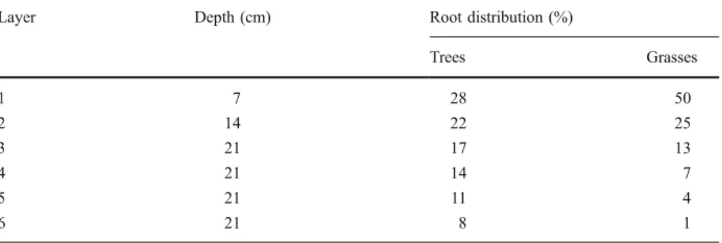
Soil hydrology is represented as a six-layer bucket model (Appendix, Table5shows the thickness of and root distribution in each soil layer). The upper three layers are filled to field capacity by rain or snow melt and reduced by transpiration, evaporation (from the upper layers), and percolation to lower layers; surplus water (beyond the storage capacity of the layer) is lost to surface runoff. The lower layers (4–6) are filled by percolation from the upper layers and reduced by plant transpiration and percolation to lower layers. Percolation from the lowest layer results in a base flow out of each simulated patch. Root distribution decreases exponentially with soil depth, whereby trees have a larger proportion of roots in deeper soil layers than grasses (Appendix, Table5). Soil properties do not differ between
the soil layers, but for our study porosity was adapted to match each site’s water holding capacity according to the pedological descriptions of the catchments (Table1).
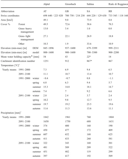
Table 1 Short description of the catchments used in the study
Alptal Grossbach Saltina Riale di Roggiasca
Abbreviation AT GB SA RR Swiss coordinates 698 640 / 223 020 700 750 / 218 230 644 220 / 129 630 733 545 / 118 160 Area [km2] 49.1 9.0 73.9 8.0 Cover % Forest 49.5 72.6 38.6 70.3 Grass–heavy management 13.0 3.4 1.0 0.0 Grass–light management 27.1 22.1 26.9 18.8 Other 10.3 1.9 33.6 10.9
Elevation (min-max) [m] DEM 845–1896 937–1600 679–3399 999–2311
Elevation (min-max) [m] model 800–1600 900–1600 700–3300 900–2200
Mean water holding capacity&
[mm] 54 43 22* 14
Catchment identification number 1251 912 867* 867
Temperature [°C]+ Yearly means 1991–2000 7.3 6.9 9.4 6.5 2091–2100 11.1 10.7 13.4 10.7 1991–2000 winter −0.4 −0.7 0.8 −1.1 spring 6.8 6.3 9.4 5.7 summer 15.3 14.8 18.1 14.7 autumn 7.4 7 9.2 6.6 2091–2100 winter 2.8 2.4 3.7 2.4 spring 10.2 9.8 12.7 9.5 summer 19.7 19.2 23.5 19.6 autumn 11.6 11.3 13.6 11.1 Precipitation [mm]+ Yearly means 1991–2000 1842 1961 760 1804 2091–2100 1650 1750 688 1631 1991–2000 winter 374 400 160 190 spring 450 477 172 409 summer 607 652 168 625 autumn 411 433 260 581 2091–2100 winter 322 343 168 301 spring 481 509 209 522 summer 451 482 119 299 autumn 397 417 192 509 +
Climate averages were done for the in the bottom of the valley, based on the spatially interpolated climate data set of Switzerland (1 ha resolution, based on DAYMET (Thornton et al.1997), data source: Land Use Dynamics, WSL Birmensdorf)
& derived from the pedological descriptions of the catchments from the FOEN (Federal Office for the Environment, Switzeralnd, catchment identification number is given in table)
* where missing, values for the Saltina valley were based on the nearby valley Goneri (distance of gauges ca. 37 km)
The LPJ-GUESS model and the closely related LPJ-DGVM have been successfully used to predict species composition as well as carbon and water fluxes at a number of different locations at point, continental and global scales (e.g. Badeck et al.2001; Smith et al.2001; Hickler et al.2004;2008; Miller et al.2008; Morales et al.2005; Koca et al.2006; Lucht et al.2002; Sitch et al.2003; Zaehle et al.2007; Wolf et al.2008). However, catchment-scale carbon and water dynamics have not been investigated to date.
2.3 Calibration of grassland management
We calibrated the LPJ-GUESS output of net ecosystem carbon exchange (NEE) to fit the NEE estimations of the grassland model PROGRASS (Lazzarotto et al. 2009) for two different management strategies (light and heavy) at two elevations (450 m and 1200 m). PROGRASS is a dynamic plot-scale model that was specifically designed to simulate grassland sites with different types of management, including fertilization and multiple harvesting. PROGRASS was validated against five years of field data from experimental sites (Oensingen, Switzerland) using two different management regimes (Lazzarotto et al. 2009); the model accurately reproduced the development of leaf area index, biomass and clover fraction under both management regimes (Lazzarotto et al.2009). Based on 25 years of observed hourly weather data (1981–2005) for the site Oensingen (450 m elevation), the weather generator LARS-WG (Semenov and Barrow2002) was used to provide synthetic time series of 100 years of daily weather variables. To derive the climate for the (virtual) high elevation site (1200 m), we assumed an increase in precipitation of +20% (moderate increase of precipitation with elevation) and a reduction in temperature of 4°C (laps rate 0.53°C/100 m). After a 2000 year spin-up to reach equilibrium conditions, PROGRASS was run for 100 years at both elevations and two management strategies, enabling us to calibrate the LPJ-GUESS model against long-term changes in NEE. The ‘heavy’ management regime included fertilization and up to five harvests per year, whereas the ‘light’ management only had three cuts and no fertilization. The mean yearly NEE was then used as a benchmark to calibrate the grass PFTs in LPJ-GUESS to fit the two management strategies. The LPJ-GUESS parameters for the root:shoot ratio, light requirements for establishment (parff), maximum transpiration (Emax), respiration coefficient (respcoeff), C:
N ratio, fraction of NPP invested in reproduction (reprfrac), low temperature limit for photosynthesis (PSlow) and the proportion of aboveground harvested material were varied
independently. In LPJ-GUESS, aboveground harvesting occurred only at the end of each simulation year, i.e. no repeated harvesting throughout the year was implemented. The parameter ranges, which were based on the parameters in two models and on an analysis of model uncertainties (Smith et al.2001, Sitch et al.2003, Zaehle et al.2005), were changed stepwise (one parameter at the time) until no further improvement of model performance compared to the benchmark was reached, i.e. Σ(NEEPROGRASS-NEELPJ-GUESS)2 was
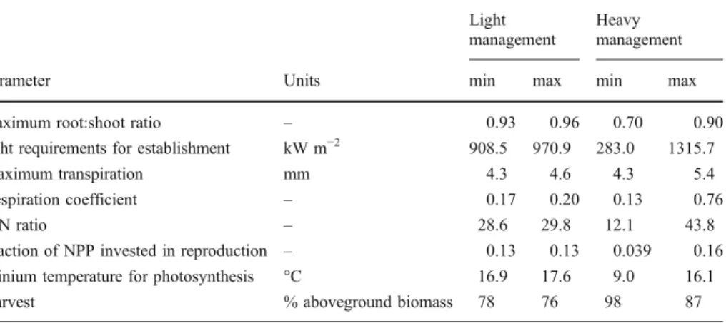
minimized. The resulting parameter set for the two management options and their uncertainties are given in Table2. The optimal parameter ranges were better constrained for the ‘light’ management. The amount of harvested material differed between the treatments and is consistent with our assumptions, i.e. the light management has a lower harvesting rate than the heavy management. Furthermore, the higher root:shoot ratio in the light management (Table2) was also an emergent feature of the PROGRASS model, where preferential root allocation was found at the sites with lower management intensity (Lazzarotto et al.2009). No parameter combination was found that gave an equally good fit for both sites and management types. Therefore, we used for the further analysis in this paper an ensemble approach, i.e. we chose the parameters randomly from the range given in
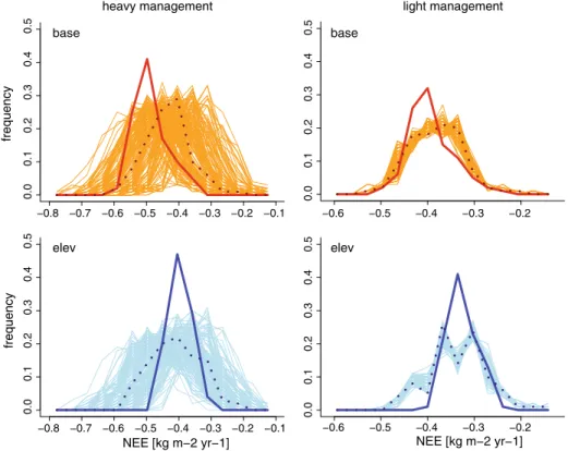
Table 2 and performed 50 runs with those parameter combinations. For the light management, LPJ-GUESS underestimated the yearly average NEE by 3% at the lower site, but overestimated NEE by 2.6% at the higher elevation (Appendix, Fig. 5). The uncertainty of the estimations at the site with light management was low compared to the uncertainty in the estimations of NEE for the more heavily managed site (Appendix, Fig. 5). For the heavy management, LPJ-GUESS resulted in an 11% underestimation of NEE at the low elevation site and an overestimation of 3.5% at the high elevation site.
2.4 Drivers
2.4.1 Climate
The model was driven by daily values of temperature, precipitation and cloud cover, and by yearly mean atmospheric CO2concentrations. The data for the four valleys were
assimilated from different data sets. Daily mean temperatures and precipitation sums from 1960–2006 were taken from the spatially interpolated climate data set of Switzerland (data source: Land Use Dynamics, WSL Birmensdorf), which has a 1 ha resolution and is based on DAYMET (Thornton et al.1997). We used the average climate for each 100 m elevation band for each catchment. For 1901–1959, we employed data from the Climate Research Unit (CRU TS 1.2, Mitchell et al.2003), whereby we used monthly temperature and precipitation anomalies averaged over the nine nearest CRU grid cells for each catchment. For 2007 to 2100, we used a regionalized climate scenario from the Institute for Atmospheric and Climate Science (IAC) at ETH Zürich (part of the ENSEMBLES project and the Swiss NCCR Climate), which is based on the A1B scenario of the IPCC AR4 (IPCC 2007). Because these data are available until 2099 only, we used the last year twice to represent the year 2100. For each valley, we used the average monthly anomaly from the nearest nine grid cells in the 10 km by 10 km grid. Anomalies were calculated from the differences in temperature and the proportional change in precipitation with the years 1961–1990 as a reference, since all three data sets had this period in common. The monthly anomalies were added to, or in case of precipitation multiplied by, the detrended daily temperature and precipitation data Table 2 Parameters space for LPJ-GUESS for light and heavy management, respectively, after calibration against PROGRASS
Light management
Heavy management
Parameter Units min max min max
maximum root:shoot ratio – 0.93 0.96 0.70 0.90
light requirements for establishment kW m−2 908.5 970.9 283.0 1315.7
Maximum transpiration mm 4.3 4.6 4.3 5.4
Respiration coefficient – 0.17 0.20 0.13 0.76
C:N ratio – 28.6 29.8 12.1 43.8
Fraction of NPP invested in reproduction – 0.13 0.13 0.039 0.16
Minium temperature for photosynthesis °C 16.9 17.6 9.0 16.1
randomly chosen from the years 1961–1990. For the control run (CTR), anomalies were assumed to be zero for temperature and 1 for precipitation, i.e. temperature and precipitation were kept constant at the level of 1961–1990.
Daily cloud cover was not available consistently from the three data sets, but it should be consistent with the amount of rainfall. Therefore, we used the observed cloud cover–rainfall relationship that was estimated from daily observations at two weather stations in Switzerland (Einsiedeln close to the Alptal catchment and Visp close to the Saltina catchment). We assumed that the relationships derived for these stations remain constant over time and are applicable in all catchments. We calculated catchment-specific cloud cover from the precipitation data for each catchment.
The CO2concentrations were based on the A1B scenario (IPCC2007), whereas for the
control run (CTR) they were kept at the year 2000 level of 369 ppm.
2.4.2 Land use
To determine current land cover, we used the areal statistic of Switzerland (Arealstatistik, BFS 2001 and the classes defined therein) and lumped this detailed land cover/land use classification into five classes: forest (classes 9–19 + abandoned land 84,86; numbering as used in the Arealstatistik), intensively used agricultural areas (class 81), less intensively used agricultural areas (classes 82,83,85,87–89,97) and unvegetated areas (urban areas: 20–69; rivers, lakes and wetlands 91–96; glaciers 90; bedrock, sand 99). We assumed that with future land use changes, the extent of the unvegetated areas will not change. This may be an underestimation for areas covered by snow, ice or bedrock, as this area may decrease under climatic change, and an overestimation for urban areas, which may expand. However, only a small part of each catchment area is covered by glaciers or urban areas today. The last class was other agriculturally used land (vineyards, fruit trees; classes 71–78) and avalanche protection areas (class 98). We assumed that this land, which constitutes only a very small proportion (0.2–0.6%) of the total catchment areas, will remain unchanged with future land use changes.
To initialize the model, we conducted a“spin-up” run, which serves to reach equilibrium in all modelled variables. To this end, we assumed that all land cover in the valleys was potential natural vegetation (PNV) prior to 1800AD, and that afterwards parts of the catchments were converted into lightly or heavily managed grasslands according to the areal statistics as described above. Although it is known that land has been used in Switzerland for a much longer time than the last 200 years, we used 1800AD as starting point for the simulation of managed land, as the years 1801–2010 were sufficient to reach a new equilibrium in vegetation carbon storage for grasslands.
To investigate the relative importance of climate and land cover change for future carbon and water relations in the catchments, we assumed that four scenarios of land use change are occurring after the year 2010: (1) land abandonment, which leads to the development of PNV, i.e. forest where this is climatically feasible. Alternatively, land use intensification was studied, i.e. in this extreme scenario all forested area was converted to grassland with either (2) light or (3) heavy management. Below the treeline, all grassland in Switzerland are actively managed as pastures or for haymaking, to prevent trees and shrubs from encroaching the open areas. Above the treeline, grasslands are natural but also mostly used as pastures or for haymaking. In this paper, we do not distinguish between pastures and hay meadows, but only between two different intensities of management (as described in Section 2.3) and refer to them as ‘light’ and ‘heavy’ managment. As a control, we assumed that (4) land use remained as observed in the areal statistics.
We assumed that all land use changes took place at one point in time, i.e. in the year 2010 (step response of the system to changes in land cover/land use). Lastly, we did not investigate the impacts of different forest management options.
2.5 Simulations
Due to the stochastic nature of tree establishment and mortality in the model, 25 replicated patches were simulated. The carbon and water fluxes were estimated along elevation gradients for each land cover type, and all combinations of possible change in land cover were simulated. For all simulations the spin-up of 900 years (corresponding to the calendar years 900–1800AD) assumed PNV. After this identical spin-up, the land cover was set to the values derived from the Swiss areal statistic (see above). For the spin-up and the years 1801–1900, we used the climate from the period 1901–1931, choosing years in random order to avoid a cyclic re-occurrence of climatic patterns.
For 1901–2010, the simulations were continued for each land use type (grassland with light management, grassland with heavy management, and PNV) using the climate as describe above. In 2010, land use change took place, whereby the four land use scenarios described above were implemented. To derive the catchment-scale response, the simulation results were then combined, weighted by the fraction of each land use type that occurred in each elevation band.
We investigated all land cover scenarios assuming either the climate change (CC) or the control scenario with no changes in climate (CTR). Additionally, we also ran simulations where temperature (T), precipitation (P), or CO2 concentrations (CO2) were changed in
isolation, in order to assess the relative importance of these drivers.
3 Results
3.1 Simulated potential natural vegetation
Simulated vegetation biomass and PFT composition fit well with the expected potential natural vegetation in all catchments. In the catchment with the longest elevation gradient (SA), PFT composition shifted from predominantly deciduous forests at the low elevations to a forest dominated by needle leaved trees (Table3). As expected, shade-intolerant trees were only found in small proportions, except at the upper treeline where they gained in importance. The treeline was found at 2200–2300 m, a realistic value for this part of the Alps (Ott 1997). Due to low water holding capacity of the soils in the SA catchment, biomass was low, varying between 6–9 kg C m−2(Table3) for the forests dominated by
needle leaved trees. The low elevation forests had a somewhat lower biomass, as rainfall was generally low in these areas. The other catchments (AT, GB and RR) were dominated by needle leaved trees as expected. At lower elevations the deciduous trees reached higher proportions, although they never dominated (results not shown). Total biomass was higher for the catchments with high water holding capacity (AT and GB, 10–16 kg C m−2) than in
catchments with the lower water holding capacity (RR, SA, 6–9 kg C m−2).
3.2 Changes in CO2concentration and climate
When land use was unchanged, total biomass was 0.6–1.2 kg C m−2 higher in 2100
scenario with no climatic change, vegetation carbon storage increased in all catchments (0.3– 0.9 kg C m−2). These changes were likely due the assumption of the CTR run, where the CO2
concentration remained at the year 2000 level, which is 369 ppm and therefore already 73 ppm higher than in 1901. The importance of CO2 concentrations in the model is also
illustrated in the CO2run, in which biomass increased considerably in all catchments (1.4–
3.0 kg C m−2, Fig.1a). Temperature changes, however, did not result in consistent changes in carbon storage. In the AT catchment, they led to a reduction of carbon storage, whereas in the other catchments the temperature-induced changes in biomass were small (Fig. 1a). The behaviour of biomass in the AT can partly be explained by the strong shift in species composition by the end of the century: the biomass of needleleaved trees was reduced (−2.2 kg C m−2), but the loss was not completely compensated by an increase in deciduous
trees (+1.1 kg C m−2). In the other valleys, the decrease of needleleaved trees was less pronounced (GB:−0.7, SA: −0.1, RR: −0.7 kg C m−2) and compensated by the increase in deciduous trees (GB: +1.4, SA: +0.4, RR: +0.6 kg C m−2). The response of biomass to precipitation changes differed between the pre-alpine catchments (AT and GB), where carbon storage increased somewhat, and SA and RR, where it was reduced slightly (Fig.1a).
Correspondingly, the changes in climate and CO2concentrations resulted in an increased
vegetation carbon uptake (15–49%) in all catchments, which was driven mainly by the CO2
Table 3 Mean biomass in the year 2000 (kg C m−2) along the elevation gradient in the Saltina valley. NE: needle leafed trees, TBS: shade-tolerant broad leafed trees, IBS: shade-intolerant broad leafed trees, GRS: grasses Elevation (m) Biomass (kg C m−2) NE TBS IBS GRS 700 0.5 2.9 0.0 0.1 800 0.5 3.8 0.0 0.0 900 1.7 3.1 0.0 0.0 1000 4.7 1.7 0.0 0.0 1100 5.5 1.7 0.0 0.0 1200 4.9 1.2 0.1 0.0 1300 6.1 1.2 0.1 0.0 1400 7.4 1.1 0.0 0.0 1500 6.9 0.5 0.1 0.0 1600 8.1 0.2 0.1 0.0 1700 8.1 0.0 0.1 0.0 1800 8.3 0.0 0.1 0.0 1900 8.3 0.0 0.0 0.0 2000 8.0 0.0 0.1 0.0 2100 6.0 0.0 0.5 0.1 2200 3.3 0.0 0.2 0.3 2300 0.0 0.0 0.8 0.3 2400 0.0 0.0 0.0 0.4 2500 0.0 0.0 0.0 0.3 2600 0.0 0.0 0.0 0.3 2700 0.0 0.0 0.0 0.2
CTR CO2 T P CC -60 -40 -20 0 20 40 60 400 200 0 400 200 0 400 200 0 400 200 0 change in AET (mm y-1) AE T (mm y -1 ) -0.08 -0.04 0.00 0.04 0.08 0.05 0.0 -0.05 0.05 0.0 -0.05 0.05 0.0 -0.05 0.05 0.0 -0.05 CTR CO2 T P CC Change in NEE (kg C m-2 y-1) NEE (kg C m -2 y -1 ) -3 -2 -1 0 1 2 3 0 6 12 0 6 12 0 6 12 0 6 12 Change in biomass (kg C m-2) Biomass (kg C m -2 ) -0.10 0.0 0.10 0.0 1.0 0.0 1.0 0.0 1.0 0.0 1.0
Change in veg. uptake (kg C m-2 y-1)
V
eg
. uptake (kg C m
-2 y -1 )
Change in soil respiration (kg C m-2 y-1)
-0.10 0.0 0.10 1.0 0 1.0 0 1.0 0 1.0 0 S oil r espiration (kg C m -2 y -1 ) AT GB SA RR -3 -2 -1 0 1 2 3 10 0
Change in soil carbon (kg C mfast -2)
Soil carbon (kg C m -2 ) fast 10 0 10 0 10 0
a)
b)
c)
d)
e)
f )
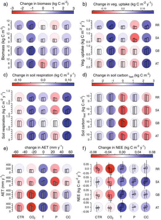
AT GB SA RR AT GB SA RRFig. 1 Climate-induced changes (land use is constant) in a biomass (kg C m−2), b vegetation carbon uptake (kg C m−2y−1), c) soil respiration (kg C m−2y−1), d fast soil carbon pool (kg C m−2), e transpiration (mm m−2y−1) and f NEE (kg C m−2y−1). The change is the difference between the mean values of 2090–2100 vs. 1990–2000. Blue colours indicate an increase, red colours a decrease. Bar plots indicate the mean absolute values in 1990–2000 (hatched bar) and 2090–2100 (empty bar), one standard deviation is indicated by the error bars. Values are given for each catchment for CTR: no climate change, CC: climate change, T: temperature change only, P: precipitation change only, CO2: CO2change only. Each row in the diagrams represents one catchment, abbreviations are explained in Table1
fertilization effect (Fig. 1b). This increase should not be compared directly to a β-value (Allen et al.1987), as the increase found here is a combination of the biomass increase (Fig.1a) and the CO2fertilization itself. The change in precipitation had a strong, negative
impact on vegetation carbon uptake, whereby the pre-alpine catchments (AT, GB) were less affected than the other two catchments. Temperature changes resulted in a differentiated response: RR and SA had a higher carbon uptake with increasing temperatures, whereas the two other catchments featured a lower uptake (Fig.1b).
Soil respiration changed consistently in all catchments (Fig. 1c). Without climatic change (control run), there was a slight reduction in soil carbon release, whereas climate change resulted in a strong increase in soil respiration (0.08–0.12 kg C m−2y−1, Fig.1c)
for two main reasons. First, the increase in soil temperature increased soil respiration (Fig.1c). This direct temperature effect resulted in the decrease of the soil carbon pools of 1.3–3.0 kg C m−2by 2100 (Fig.1d). Second, litter input to the soil increased due to the higher productivity, and as most of the litter is decomposed within a few years, soil respiration increased. The importance of litter input for soil respiration was nicely illustrated in the simulation where only the CO2 fertilization effect was considered and
the fast soil carbon pool increased by more than 1 kg C m−2(Fig.1d) and soil respiration increased as well. Changes in precipitation alone led to a decrease in soil respiration, whereby the dry catchments (SA, RR) showed a stronger response compared to the wet catchments (Fig.1c).
Simulated changes in transpiration confirmed the expectation that on the one hand higher temperatures result in an increase of energy available for transpiration (Fig.1e), and on the other hand the CO2increase and the reduced precipitation result in a reduction in
transpiration. Temperature was the main driver for the transpiration changes under future climatic conditions, except for the SA valley where the reduction in transpiration due to the change in precipitation was quite strong (Fig.1e).
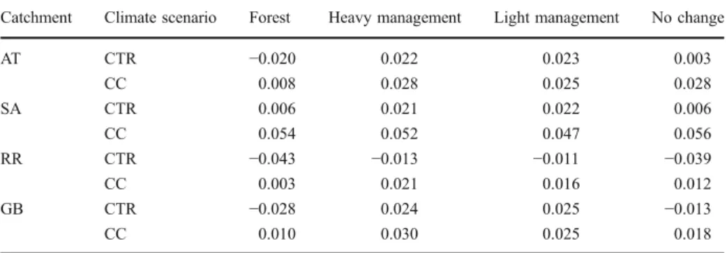
The net effect of climatic change on the catchment-scale carbon balance showed that between 2090 and 2100 all catchments were carbon sources, as average NEE was positive (Table4). Considering the sink / source strength by the end of the century, temperature and precipitation changes resulted in an increase of carbon source in all catchments, whereas the CO2-fertization had the opposite effect (Fig.1f). This latter effect was not strong enough to
compensate for the increase in C-loss due to changes in temperature and precipitation. The
Table 4 Mean NEE for the period 2090–2100 (kg C m−2y−1) for the four catchments. Positive values indicate a carbon source, negative values a carbon sink. CTR is the control run without climatic change, and CC is the climate change run. For catchments abbreviations, see Table1
Catchment Climate scenario Forest Heavy management Light management No change
AT CTR −0.020 0.022 0.023 0.003 CC 0.008 0.028 0.025 0.028 SA CTR 0.006 0.021 0.022 0.006 CC 0.054 0.052 0.047 0.056 RR CTR −0.043 −0.013 −0.011 −0.039 CC 0.003 0.021 0.016 0.012 GB CTR −0.028 0.024 0.025 −0.013 CC 0.010 0.030 0.025 0.018
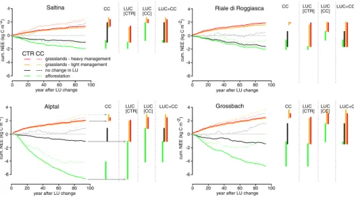
cumulative effect of climate change since 2010 also showed that by 2100 all catchments would turn from sinks to sources of carbon (Fig.2, dotted black lines).
3.3 Land use change
Reforestation As expected, carbon stored in biomass increased strongly (1.1–6.0 kg C m−2)
when the catchments were reforested (PNV). Soil carbon storage increased as well (0.4– 0.9 kg C m−2, Fig.3a) compared to the control run (0.3–0.4 kg C m−2). Correspondingly, a strong carbon sink was evident for the AT and the GB catchments, whereas in the SA and RR reforestation resulted in a smaller sink (Figs.2and 3d).
Deforestation The removal of all forests led to a large loss of vegetation biomass (4.0– 8.8 kg C m−2, results not shown), as more carbon is stored in tree than in grass biomass. The soil carbon pool decreased by 0.6–1.7 kg C m−2, whereby carbon loss was higher in the
forest-rich catchments (Fig. 3a). Soil respiration decreased markedly after deforestation (Fig.3c) because of the strongly reduced litter input. However, vegetation carbon uptake differed comparatively little between the land use scenarios (Fig.3b). When carbon storage was considered (Figs.2and3d), deforestation always resulted in a loss of carbon from the catchments (Figs.2and 3d). A decrease in transpiration was simulated after deforestation (Fig.4), due to the shallower root system of grasses compared to trees.
Management intensity Whether the grasslands were managed more or less intensively (light or heavy) had little impact on carbon storage in the catchment (Fig.2, orange vs. red lines). More carbon was taken up by the vegetation when land was heavily managed (Fig.2), but
20 40 60 80 2 4 0 -2 -4 -6
year after LU change
0 100 CC LUC [CTR] LUC [CC] LUC+CC 2 4 0 -2 -4 -6 20 40 60 80 year after LU change
0 100 CC LUC [CTR] LUC [CC] LUC+CC Alptal Grossbach
grasslands - heavy management grasslands - light management no change in LU afforestation CTR CC 2 4 0 -2 -4 -6 cum. NEE (kg C m -2) cum. NEE (kg C m -2) cum. NEE (kg C m -2) cum. NEE (kg C m -2) 20 40 60 80
year after LU change
0 100 CC LUC [CTR] LUC [CC] LUC+CC 2 4 0 -2 -4 -6
Saltina Riale di Roggiasca CC LUC [CTR]
LUC [CC] LUC+CC
20 40 60 80 year after LU change
0 100
Fig. 2 Cumulative change in NEE (kg C m−2) since 2010 for all catchments. Different colours indicate different land use scenarios. Solid lines denote runs with the control scenario, dotted lines those under the climate change scenarios. Bars represent cumulative NEE until 2100. CC: only climate change is considered (the two upper grey lines in the Alptal catchment are guidance lines for illustration); LUC[CTR]: the effect of land use change when climate is not changing (the two lower grey lines in the Alptal catchment are guidance lines for illustration); LUC[CC]: the difference between land use change scenarios under climate changed; LUC + CC: combined impact of land use and climate change, i.e. compared to control run with no climate change
-0.3 -0.2 -0.1 0.0 0.1 0.2 0.3 -0.15 -0.10 -0.05 0.00 0.05 0.10 0.15 -6 -4 -2 0 2 4 6 GB AT SA RR -2 -1 0 1 2
a) fast soil pool [ kg Cm y ]-2 -1
b) vegetation carbon uptake [ kg Cm y ]-2 -1
c) soil respiration[ kg Cm y ]-2 -1 d) cumulative NEE [ kg Cm y ]-2 -1 Grassl. light Grassl. heavy No LUC Forest Grassl. light Grassl. heavy No LUC Forest Grassl. light Grassl. heavy No LUC Forest Grassl. light Grassl. heavy No LUC Forest
Fig. 3 Changes in a fast soil pool (kg C m−2), b vegetation carbon uptake (kg C m−2y−1), c soil respiration (kg C m−2y−1) and d cumulative NEE (kg C m−2) due to land use change for all catchments. Climate was assumed be constant. Values represent the difference between means in 2090–2100 and 1990– 2000. Each row shows a different land use scenario (“No LUC”: no land use change;“Grassl. light”: deforestation + light grassland management;“Grassl. heavy”: deforestation + heavy grassland management;“Forest”: catchment reforested). The rows show the four catchments, abbre-viations in Table1. Red colours indicate a decrease, blue colours an increase in value. For d, red values indicate carbon uptake, whereas blue colours indicate a carbon loss from the catchment. For catchment abbreviations, cf. Table1
as most of the aboveground fraction of this carbon was harvested, the higher uptake did not result in an increase of soil carbon storage (Fig.3a).
3.4 Interaction of climate and land use changes
Looking at the cumulative NEE over the next 90 years, several patterns stand out (Fig.2). On the one hand, the land use scenarios employed here had a stronger impact on carbon storage than the climate change scenario. On the other hand, climate change generally had a smaller effect on carbon storage on actively managed grassland systems compared to a management where parts or the whole catchment were forested (Fig.2, CC).
In all catchments only reforestation led to a carbon sink when climate was changing (Fig.2, dotted green lines). All other land use scenarios turned the catchment into carbon sources under climate change, except for RR, where only small changes in carbon storage were observed even when land use was kept constant. Importantly, only in the AT the carbon sink was considerable (cumulative NEE larger than 2 kg C m−2) when climatic change was taken into account. In all other catchments, reforestation did not strongly increase catchment sink activity. Furthermore, after approximately 50 years the cumulative NEE did not change in any of the catchments under the reforestation scenario. Cumulative NEE even decreased somewhat for all catchments by the end of the century. Average NEE over the years 2090– 2100 indicates that all catchments were carbon sources in that period (Table4).
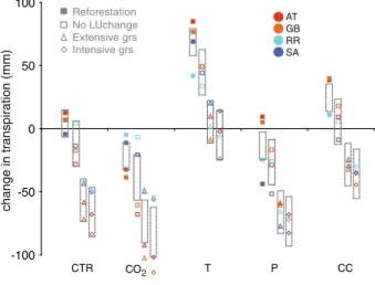
As expected from the lower transpiration of grasses due to their shallow root system, deforestation resulted in a reduction in transpiration, whereas afforestation resulted in an increase (Fig.4). The change in transpiration was surprisingly small under climatic change, as the temperature induced increase in transpiration was compensated by the decrease in transpiration due to precipitation and CO2.
There was a strong interaction between the effects of land use change and climate change regarding the water balance (Fig.4). Transpiration responses to climate change became more similar between catchments when they were deforested, but less similar when they were reforested. Interestingly, under the control scenario (CTR) catchment transpiration was more similar between catchments when reforestation was assumed (Fig.4, CTR), whereas under the climate change scenario, the response of catchments under the reforestation scenario was less similar when compared to the other land use change scenarios. When the catchments were
Reforestation No LUchange Extensive grs Intensive grs -100 -50 0 50 100 CTR CO2 T P CC change in transpiration (mm) AT GB RR SA Fig. 4 Changes in transpiration
(mm) are shown as the differ-ences in average values between 2090–2100 and 1990–2000. The catchments are represented by different colours (for abbrevi-ations cf. Table1). The land use scenarios are represented by different symbols. The size of the grey boxes measures the variation between catchments for each land use type under the CTR climate. They are copied to the other scenarios to assist the comparison of the scenario variation and the variation under CTR climate
covered by forest, each of the climate change components (temperature, precipitation, CO2) led
to a strongly different transpiration response. For example, the CO2 response was more
pronounced in the AT and GB catchments, whereas CO2 had only minor impacts on
transpiration in the SA and RR catchments (Fig.4). Even more striking was the difference in precipitation responses. For example, the decrease in precipitation had almost no influence on transpiration in the AT and GB catchments, but it led to much lower transpiration for the catchments SA and RR (Fig.4).
When land use was changed to grassland, the transpiration response to climate change became more similar than in the run with constant climate (Fig.4). Higher temperature led to a similar transpiration increase in all catchments, whereas the CO2response decreased
transpiration to a larger extent in the AT and GB than in the RR and SA catchments. Importantly, transpiration was reduced strongly when precipitation changes were consid-ered, and thus catchment responses became more similar, which was likely the reason that combined CC responses were quite similar between the different catchments in the grassland management scenarios.
4 Discussion
4.1 Carbon cycle
Climate change turned three out of four catchments into carbon sources when land use remained as observed today (Figs. 1 and 2), but the drivers responsible for this change differed. In the two pre-alpine catchments AT and GB, the increase in carbon uptake due to increased temperatures and higher CO2 concentrations (Fig.1a,c) was counteracted by an
increase in decomposition due to higher soil temperatures (Fig.1b). A temperature-driven increase in decomposition was as also found in other studies as long as moisture is not limiting (e.g., Bellamy et al. 2005; Borken et al. 2006; Hibbard et al. 2005). In the two catchments that feature terrain above the current treeline (SA and RR), the temperature-induced upward shift of the treeline allowed forests to grow at higher elevations, and hence carbon storage increased. Such shifts with temperature have been observed widely (e.g., Harsch et al.2009; Gehrig-Fasel et al.2007; Kullman2002; Shiyatov et al.2007) and are expected to continue (cf. Theurillat and Guisan 2001; Didion et al. in press). In our simulations this increase in carbon storage was partly offset by an increase in drought risk at lower elevations. Especially in the dry valley SA, the combination of low summer precipitation with low soil water holding capacity led to a decrease in forest cover at the lower, dry elevations. This is in agreement with studies that showed an increase in drought stress and/or drought induced tree mortality in the Valais, where the SA catchment is located (Bigler et al.2006; Rigling et al.2002) and with other modelling studies that demonstrated a high risk of drought-induced forest decline (Didion et al.in press; Zierl and Bugmann 2007). Only in the RR valley, the increase in carbon storage due to shifts in the upper treeline was large enough to compensate fully for the increase in soil respiration, leading to only small changes in carbon storage in this catchment. Due to differences in plant functional type composition, climate and topography, the response of carbon storage to climatic changes differed widely between catchments and illustrate that in highly complex terrain such as the European Alps, high-resolution studies are needed, and simple response functions cannot be expected (Daly et al.2010).
Any intensification of land use turned the catchments into carbon sources (Fig. 2), whereby in addition to the expected above ground loss due to deforestation, the reduced
litter input due to harvesting lead to a loss in soil carbon storage (Fig.3). Such losses in soil carbon after deforestation are in agreement with measurements both globally (Guo and Gifford2002) and in the UK (Cannell et al.1999), although some studies of pastures (Guo and Gifford2002), dry regions in Africa (Albrecht and Kandji2003) or loess areas in China (Chen et al. 2007) found that grassland soils store more or at least similar amounts of carbon as forests soils. It is important to notice that not only the immediate change in aboveground biomass contributes to the loss of carbon in the catchment, but also changes in litter input. Thus, land use effects were similar in direction between the catchments, but larger changes were found in carbon storage in the catchments with more extensive forest cover (GB and RR) due to the larger impact of deforestation.
Under the climate change scenario, only the radical change of complete afforestation led to a carbon sink in the catchments. Even more importantly, this sink is not stable under the climate change scenario as carbon uptake came to a halt around 2050 (cumulative NEE in Fig.2) and the trend might even be reversed by the end of the century (Fig.2, valleys GB, SA, RR). In our modelling study, land use change was typically more important for catchment carbon storage than climatic change. In the managed grasslands, soil carbon storage decreased in the long term as result of the repeated removal of aboveground biomass (harvesting). For this land use scenario, the additional change of climate had only comparatively little effect on carbon storage as the change in litter input was more important. For the other extreme case, i.e. the afforestation of all suitable areas in the catchment, climate had the strongest influence on carbon storage, resulting in a reduction of carbon sink strength for all catchments over time. Our results of the changes of belowground carbon storage differed from global results based on the LPJmL model (Müller et al.2007), where land use change mainly affected the aboveground carbon pool. However, as Müller et al. (2007) used a different approach by exploring three climate change scenarios (A2, B1, B2) and land use scenarios consistent with the underlying IPCC storylines, they were not able to separate the effects of climate change and land use change, as we here.
4.2 Water cycle
We found a temperature-induced increase and a CO2-induced decrease in transpiration
(Fig.4), which is in agreement with observations (e.g. Farley et al.2005; Leuzinger and Körner2007). Our study also showed that the increase in forest cover led to an increase in transpiration, as found in Germany (Wattenbach et al. 2007) and also reflected in the runoff decrease found in a meta-analysis (Farley et al.2005). Also for transpiration the interactions between land use and climate change need to be considered (Fig. 4). Interestingly, we found that the transpiration responses to climate change were more similar between catchments when management was intensified, but less similar when they were reforested. This was due to the structurally more homogenous grassland vegetation, where both aboveground (leaves) and belowground (roots) responses were similar, whereas the forest ecosystems were more heterogeneous due to the differences in ecosystem structure as a consequence of strongly different sizes of individuals and a different tree species composition. These opposite responses of transpiration under climate change needs to be considered in climate models, as it cannot be assumed that the vegetation feedback remains similar across large areas (catchments and beyond). If catchments are forest-covered and have a low mean water holding capacity (RR, SA), a strong negative impact on transpiration may occur when precipitation decreases, whereas there may be no response of catchments with higher water holding capacity (AT, GB). In
case of grassland-covered catchments, however, the precipitation-induced response may be strong and in our case surprisingly similar across catchments, indicating that the shallow rooting system of grasses in the model prevents them from tapping deeper soil layers.
4.3 Limitations
As all model-based estimates, our approach has limitations. We calibrated the LPJ-GUESS model against outputs from the model PROGRASS (Lazzarotto et al.2009), which has limitations on its own but performed well when used for grasslands with different management intensity in Switzerland (Lazzarotto et al.2009). Using PROGRASS enabled us to fit our model against long-term simulations (here, 100 years) which is needed as the model output should represent long-term trends in the first place, rather than short-term (intra-annual) responses. Interestingly, our calibration against NEE was satisfactory for grasslands with light management, but less so for the heavy management. This indicates that for improving NEE predictions for more heavily used areas, repeated harvesting and fertilization, i.e. a coupled C:N cycle, need to be included explicitly in LPJ-GUESS. Although LPJ-GUESS did not include nitrogen fertilization here, differences in vegetation carbon uptake between the two management scenarios were indirectly considered due to the calibration against PROGRASS results that considered different fertilization regimes. Additionally, we expect that in Switzerland strong anthropogenic nitrogen deposition will continue in the future such that none of the considered catchment will become nitrogen limited. Furthermore, as the differences in responses between grassland management scenarios were small in the four catchments, especially when compared to other land use types, we still suggest that our conclusions regarding the differences between grassland management and other land use changes are valid.
We used only one climate change scenario and compared it to different land use scenarios; while other climate scenarios would have led to differences in the absolute values of the simulated responses, the qualitative nature of our results, especially regarding the importance of the interaction between land use and climate change, would remain evident also with other climate scenarios. Although it is very unlikely that land use will change as extremely as we assumed here, i.e. complete deforestation or reforestation of the catchments, these extreme scenarios span the range of possible responses to land use changes in the catchments. As the estimated responses to land use change were strong, we expect that also smaller changes in land use would still have discernible impacts on both carbon storage and transpiration.
The spatial heterogeneity of soil properties within the catchments clearly influences our results, especially for the two catchments with low soil water holding capacity (SA, RR); this should therefore be investigated more thoroughly. We restricted vegetation cover to areas where vegetation (mainly alpine pasture) is present today, which may have led to an underestimation of vegetation response particularly in the SA valley, since at high elevations vegetation may colonize new areas. While this is important from a biodiversity point of view, we expect that growth and hence carbon uptake will still be low in these areas.
Although forest management and site history are important for soil carbon storage (Jandl et al.2007; Ågren et al.2007; Liski et al.2002; Gimmi et al.2009), we did not evaluate specific forest management practices here, as the focus was on the importance of broad changes of land cover. Also the effects of climate change on litter quality and litter composition (Cornelissen et al.2007; Cornwell et al.2008) were not considered explicitly. Still, our finding that the amount of litter input is highly important would be unlikely to change if aspects of litter quality were included in the model.
5 Conclusion
We provide evidence that the interactions between the carbon and the water cycle are quite important for determining catchment responses to changes in climate and land use; that the overall response can vary strongly between different catchments; and that these responses need to be studied in detail, otherwise erroneous conclusions may arise regarding ecosystem responses to global change in complex mountain terrain.
Specifically, we showed that only reforestation could lead to enhanced carbon storage in the catchments whereas the other land use scenarios resulted in carbon release from all catchments under climatic change. Furthermore, if plant water supply was limiting either due to low precipitation (SA) and/or low water holding capacity of the soil (SA, RR), the responses to land use change and to climate change were much smaller.
There are important interactions between land use change and climatic change, i.e. the additional carbon storage due to afforestation was often only temporary. After 2050, the carbon accumulation stopped, and in some catchments carbon was even released due to further changes in climate. Conversely, deforestation leads to a decrease in soil carbon storage due to changes in litter input, in addition to the immediate carbon loss induced by the removal for the trees.
Land use change influenced transpiration directly, but it also interacted with climate change. Forested land responded highly differently to climatic changes, reflecting the species composition, topography and water holding capacity of the respective catchments, whereas grasslands responded more similarly, almost independent of catchment properties. Thus, studies that address the climatic feedbacks from ecosystems should consider these different responses in transpiration, particularly because the response is persisting, unlike carbon storage, which levels off within a few decades.
Acknowledgements We thank the Institute for Atmospheric and Climate Science (AIC) at ETHZ and the Land Use Dynamics Group, WSL Birmensdorf for providing climate data. We furthermore acknowledge NCCR climate and the EU-FP7 project ACQWA for financial contribution. We thank B. Smith (Lund University, Sweden) for providing the source code of the LPJ-GUESS model.
Appendix
Table 5 Soil depth (cm) and root distribution of trees and grasses (%) for each soil layer in LPJ-GUESS
Layer Depth (cm) Root distribution (%)
Trees Grasses 1 7 28 50 2 14 22 25 3 21 17 13 4 21 14 7 5 21 11 4 6 21 8 1
References
Ågren GI, Hyvönen R, Nilsson T (2007) Are Swedish forest soils sinks or sources for CO2—model analyses based on forest inventory data. Biogeochemistry 82:217–227
Albrecht A, Kandji ST (2003) Carbon sequestration in tropical agroforestry systems. Agric Ecosyst Environ 99:15–27
Allen LHJ, Boote KJ, Jones JW, Jones PH, Valle RR, Acock B, Rogers HH, Dahlman RC (1987) Response of vegetation to rising carbon dioxide: photosynthesis, biomass, and seed yield of soybean global biogeochem. Cycles 1:1–14
Archaux F, Wolters V (2006) Impact of summer drought on forest biodiversity: what do we know? Ann For Sci 63:645–652
Badeck F-W, Lischke H, Bugmann H, Hickler T, Honninger K, Lasch P, Lexer MJ, Mouillot F, Schaber J, Smith B (2001) Tree species composition in European pristine forests: comparison of stand data to model predictions. Clim Chang 51:307–347
Bellamy PH, Loveland PJ, Bradley RI, Lark RM, Kirk GJD (2005) Carbon losses from all soils across England and Wales 1978–2003. Nature 437:245–248
BFS (Bundesamt für Statistik) (2001) Arealstatistik der Schweiz 1992/1997. Neuchatel
Bigler C, Bräker OU, Bugmann H, Dobbertin M, Rigling A (2006) Drought as an inciting mortality factor in scots pine stands of the Valais, Switzerland. Ecosystems 9:330–343
−0.8 −0.7 −0.6 −0.5 −0.4 −0.3 −0.2 −0.1 0.0 0.1 0.2 0.3 0.4 0.5 −0.8 −0.7 −0.6 −0.5 −0.4 −0.3 −0.2 −0.1 0.0 0.1 0.2 0.3 0.4 0.5 NEE [kg m−2 yr−1] −0.6 −0.5 −0.4 −0.3 −0.2 0.0 0.1 0.2 0.3 0.4 0.5 −0.6 −0.5 −0.4 −0.3 −0.2 0.0 0.1 0.2 0.3 0.4 0.5 NEE [kg m−2 yr−1] heavy management frequency frequency light management base base elev elev
Fig. 5 Frequency of NEE (kg C m−2y−1) for 100 simulation years for the benchmark simulation by PROGRASS (thick line) and the LPJ-GUESS ensembles (thin lines). The LPJ-GUESS mean is shown as a dotted line. Colours indicate the elevation: orange/red indicates runs at low elevation (base) and blue colours indicate runs at the high elevation site (elev). Heavy and light management are shown in the different columns
Boix-Fayos C, Vente J et al (2009) Soil carbon erosion and stock as affected by land use changes at the catchment scale in Mediterranean ecosystems. Agric Ecosyst Environ 133:75–85
Borken W, Savage K, Davidson EA, Trumbore SE (2006) Effects of experimental drought on soil respiration and radiocarbon efflux from a temperate forest soil. Glob Chang Biol 12:177–193
Brovkin V, Claussen M, Driesschaert E, Fichefet T, Kicklighter D, Loutre MF, Matthews HD, Ramankutty N, Schaeffer M, Sokolov A (2006) Biogeophysical effects of historical land cover changes simulated by six Earth system models of intermediate complexity. Clim Dyn 26:587–600
Brown AE, Zhang L, McMahon TA, Western AW, Vertessy RA (2005) A review of paired catchment studies for determining changes in water yield resulting from alterations in vegetation. J Hydrol 310:28–61
Cannell MGR, Milne R, Hargreaves KJ, Brown TAW, Cruickshank MM, Bradley RI, Spencer T, Hope D, Billett MF, Adger WN, Subak S (1999) National inventories of terrestrial carbon sources and sinks: the UK experience. Clim Chang 42:505–530
Chen LD, Gong J, Fu BJ, Huang ZL, Huang YL, Gui LD (2007) Effect of land use conversion on soil organic carbon sequestration in the loess hilly area, loess plateau of China. Ecol Res 22:641–648 Cornelissen JHC, van Bodegom PM, Aerts R, Callaghan TV, van Logtestijn RSP, Alatalo J, Stuart CF, Gerdol
R, Gudmundsson J, Gwynn-Jones D, Hartley AE, Hik DS, Hofgaard A, Jonsdottir IS, Karlsson S, Klein JA, Laundre J, Magnusson B, Michelsen A, Molau U, Onipchenko VG, Quested HM, Sandvik SM, Schmidt IK, Shaver GR, Solheim B, Soudzilovskaia NA, Stenstrom A, Tolvanen A, Totland O, Wada N, Welker JM, Zhao X (2007) Global negative vegetation feedback to climate warming responses of leaf litter decomposition rates in cold biomes. Ecol Lett 10:619–627
Cornwell WK, Cornelissen JHC, Amatangelo K, Dorrepaal E, Eviner VT, Godoy O, Hobbie SE, Hoorens B, Kurokawa H, Pérez-Harguindeguy N, Quested HM, Santiago LS, Wardle DA, Wright IJ, Aerts R, Allison SD, Bodegom PV, Brovkin V, Chatain A, Callaghan TV, Díaz S, Garnier E, Gurvich DE, Kazakou E, Klein JA, Read J, Reich PB, Soudzilovskaia NA, Vaieretti MV, Westoby M (2008) Plant species traits are the predominant control on litter decomposition rates within biomes worldwide. Ecol Lett 11:1065–1071
Daly C, Bachelet D, Lenihan JM, Neilson RP, Parton W, Ojima D (2000) Dynamic simulation of tree-grass interactions for global change studies. Ecol Appl 10:449–469
Daly C, Conklin DR, Unsworth MH (2010) Local atmospheric decoupling in complex topography alters climate change impacts. Int J Climatol 30:1857–1864
Didion M, Kupferschmid AD, et al. (in press) Ungulate herbivory modifies the effects of climate change on mountain forests. Climatic Change doi:10.1007/s10584-011-0054-4
Eugster W, Cattin R (2007) Evapotranspiration and energy flux differences between a forest and a grassland site in the subalpine zone in the Bernese Oberland. Die Erde 138:237–256
Farley KA, Jobbagy EG, Jackson RB (2005) Effects of afforestation on water yield: a global synthesis with implications for policy. Glob Chang Biol 11:1565–1576
Fuhrer J, Beniston M, Fischlin A, Ch F, Goyette S, Jasper K, Ch P (2006) Climate risks and their impact on agriculture and forests in Switzerland. Clim Chang V79:79–102
Gehrig-Fasel J, Guisan A, et al. (2007) Tree line shifts in the Swiss Alps: climate change or land abandonment? Journal of Vegetation Science 571–582
Gerten D, Schabhoff S, Haberlandt U, Lucht W, Sitch S (2004) Terrestrial vegetation and water balance— hydrological evaluation of a dynamic global vegetation model. J Hydrol 286:249–270
Gimmi U, Wolf A et al (2009) Quantifying disturbance effects on vegetation carbon pools in mountain forests based on historical data. Reg Environ Chang 9:121–130
Guo LB, Gifford RM (2002) Soil carbon stocks and land use change: a meta analysis. Pages 345–360 Harsch MA, Hulme PE et al (2009) Are treelines advancing? A global meta-analysis of treeline response to
climate warming. Ecol Lett 12:1040–1049
Hibbard KA, Law BE, Reichstein M, Sulzman J (2005) An analysis of soil respiration across northern hemisphere temperate ecosystems. Biogeochemistry 73:29–70
Hickler T, Smith B, Sykes MT, Davis MB, Sugita S, Walker K (2004) Using a generalized vegetation model to simulate vegetation dynamics in northeastern USA. Ecology 85:519–530
Hickler T, Smith B, Prentice IC, Mjofors K, Miller P, Arneth A, Sykes MT (2008) CO2 fertilization in temperate FACE experiments not representative of boreal and tropical forests. Glob Chang Biol 14:1531–1542
Huber UM, Bugmann HKM et al (2005) Global change and mountain regions. An overview of current knowledge. Advances in Global Change Research. Dordrecht, Springer
IPCC (2007) Climate change 2007: the physical science basis - summary for policymakers, IPCC WGI Fourth Assessment Report
Jandl R, Lindner M, Vesterdal L, Bauwens B, Baritz R, Hagedorn F, Johnson DW, Minkkinen K, Byrne KA (2007) How strongly can forest management influence soil carbon sequestration? Geoderma 137:253– 268
Koca D, Smith B et al (2006) Modelling regional climate change effects on potential natural ecosystems in Sweden. Clim Chang 78:381–406
Kullman L (2002) Rapid recent range-margin rise of tree and shrub species in the Swedish Scandes. J Ecol 90:68–77
Laurent M, Antoine N, Joel G (2003) Effects of different thinning intensities on drought response in Norway spruce (Picea abies (L.) Karst.). For Ecol Manag 183:47–60
Lazzarotto P, Calanca P, Fuhrer J (2009) Dynamics of grass-clover mixtures—an analysis of the response to management with the PROductive GRASsland Simulator (PROGRASS). Ecol Model 220:703–724 Leuzinger S, Zotz G, Asshoff R, Körner C (2005) Responses of deciduous forest trees to severe drought in
Central Europe. Tree Physiol 25:641–650
Leuzinger S, Körner C (2007) Water savings in mature deciduous forest trees under elevated CO2. Glob Chang Biol 13:2498–2508
Liski J, Perruchoud D, Karjalainen T (2002) Increasing carbon stocks in the forest soils of western Europe. For Ecol Manag 169:159–175
Lloyd J, Taylor JA (1994) On the temperature dependence of soil respiration. Funct Ecol 8:315–323 Lucht W, Prentice IC, Myneni RB, Sitch S, Friedlingstein P, Cramer W, Bousquet P, Buermann W, Smith B
(2002) Climatic control of the high-latitude vegetation greening trend and Pinatubo effect. Science 296:1687–1689
Mackay DS, Band LE (1997) Forest ecosystem processes at the watershed scale: dynamic coupling of distributed hydrology and canopy growth. Hydrol Process 11:1197–1217
Miller PA, Giesecke T, Hickler T, Bradshaw RHW, Smith B, Seppa H, Valdes PJ, Sykes MT (2008) Exploring climatic and biotic controls on Holocene vegetation change in Fennoscandia. J Ecol 96:247–259 Mitchell TD, Carter TR, Jones PD, Hulme M, New M (2003). A comprehensive set of climate scenarios for
Europe and the globe. Tyndall Centre Working Paper 55
Morales P, Sykes MT, Prentice CI, Smith P, Smith B, Bugmann H, Zierl B, Friedlingstein P, Viovy N, Sabate S, Sanchez A, Pla E, Gracia CA, Sitch S, Arneth A, Ogee J (2005) Comparing and evaluating process-based ecosystem model predictions of carbon and water fluxes in major European forest biomes. Glob Chang Biol 11:1–23
Müller C, Eickhout B, Zaehle S, Bondeau A, Cramer W, Lucht W (2007) Effects of changes in CO2, climate, and land use on the carbon balance of the land biosphere during the 21st century. J Geophys Res-Biogeosci 112:G02032
Ott E (1997) Gebirgsnadelwälder. Paul Haupt Verlag
Ponton S, Flanagan LB, Alstad KP, Johnson BG, Morgenstern KAI, Kljun N, Black TA, Barr AG (2006) Comparison of ecosystem water-use efficiency among Douglas-fir forest, aspen forest and grassland using eddy covariance and carbon isotope techniques. Glob Chang Biol 12:294–310
Rowell D, Jones R (2006) Causes and uncertainty of future summer drying over Europe. Clim Dyn 27:281– 299
Rigling A, Braker O et al (2002) Intra-annual tree-ring parameters indicating differences in drought stress of Pinus sylvestris forests within the Erico-Pinion in the Valais (Switzerland). Plant Ecol 163:105–121 Schmid S, Thurig E et al (2006) Effect of forest management on future carbon pools and fluxes: a model
comparison. For Ecol Manag 237:65–82
Scott RL, Huxman TE, Williams DG, Goodrich DC (2006) Ecohydrological impacts of woody-plant encroachment: seasonal patterns of water and carbon dioxide exchange within a semiarid riparian environment. Glob Chang Biol 12:311–324
Semenov MA, Barrow EM (2002) LARS-WG - A stochastic weather generator for use in climate impact studies Seneviratne S, Lüthi D, Litschi M, Schär C (2006) Land-atmosphere coupling and climate change in Europe.
Nature 443:205–209
Shiyatov SG, Terentev MM, Fomin VV, Zimmermann NE (2007) Altitudinal and horizontal shifts of the Upper Boundaries of open and closed forests in the Polar Urals in the 20th century. Russ J Ecol 38:223– 227
Sitch S, Smith B, Prentice IC, Arneth A, Bondeau A, Cramer W, Kaplan JO, Levis S, Lucht W, Sykes MT, Thonicke K, Venevsky S (2003) Evaluation of ecosystem dynamics, plant geography and terrestrial carbon cycling in the LPJ dynamic global vegetation model. Glob Chang Biol 9:161–185
Smith B, Prentice IC, Sykes MT (2001) Representation of vegetation dynamics in the modelling of terrestrial ecosystems: comparing two contrasting approaches within European climate space. Glob Ecol Biogeogr 10:621–637
Tenhunen J, Geyer R, et al (2009) Influences of changing land use and CO2 concentration on ecosystem and landscape level carbon and water balances in mountainous terrain of the Stubai Valley, Austria. Fall Annual Meeting of the American-Geophysical-Union, San Francisco, CA
Theurillat JP, Guisan A (2001) Potential impact of climate change on vegetation in the European Alps: a review. Clim Chang 50:77–109
Thornton PE, Running SW et al (1997) Generating surfaces of daily meteorological variables over large regions of complex terrain. J Hydrol 190:214–251
van Dijk AIJM, Keenan RJ (2007) Planted forests and water in perspective. For Ecol Manag 251:1–9 Wattenbach M, Zebisch M et al (2007) Hydrological impact assessment of afforestation and change in
tree-species composition - A regional case study for the Federal State of Brandenburg (Germany). J Hydrol 346:1–17
Wolf A, Callaghan T, Larson K (2008) Future changes in vegetation and ecosystem function of the Barents Region. Clim Chang 87:51–73
Zaehle S, Sitch S, Smith B, Hatterman F (2005) Effects of parameter uncertainties on the modeling of terrestrial biosphere dynamics. Glob Biogeochem Cyc 19:GB3020
Zaehle S, Bondeau A, Carter T, Cramer W, Erhard M, Prentice I, Reginster I, Rounsevell M, Sitch S, Smith B, Smith P, Sykes M (2007) Projected changes in Terrestrial Carbon Storage in Europe under climate and land-use change, 1990–2100. Ecosystems 10:380–401
Zierl B, Bugmann H (2007) Sensitivity of carbon cycling in the European Alps to changes of climate and land cover. Clim Chang 85:195–212