HAL Id: hal-01175587
https://hal-univ-perp.archives-ouvertes.fr/hal-01175587
Submitted on 2 Mar 2021
HAL is a multi-disciplinary open access
archive for the deposit and dissemination of
sci-entific research documents, whether they are
pub-lished or not. The documents may come from
teaching and research institutions in France or
abroad, or from public or private research centers.
L’archive ouverte pluridisciplinaire HAL, est
destinée au dépôt et à la diffusion de documents
scientifiques de niveau recherche, publiés ou non,
émanant des établissements d’enseignement et de
recherche français ou étrangers, des laboratoires
publics ou privés.
Heuristic shape optimization of baffled fluid distributor
for uniform flow distribution
Lingai Luo, Min Wei, Yilin Fan, Gilles Flamant
To cite this version:
Lingai Luo, Min Wei, Yilin Fan, Gilles Flamant. Heuristic shape optimization of baffled fluid
dis-tributor for uniform flow distribution. Chemical Engineering Science, Elsevier, 2015, 123, pp.542-556.
�10.1016/j.ces.2014.11.051�. �hal-01175587�
Luo, L., Wei, M., Fan, Y., & Flamant, G. (2015). Heuristic shape optimization of
1
baffled fluid distributor for uniform flow distribution. Chemical Engineering Science,
2
123, 542–556. https://doi.org/10.1016/j.ces.2014.11.051.
3
4
Heuristic Shape Optimization of Baffled Fluid Distributor for
5
Uniform Flow Distribution
6
Lingai LUOa*, Min WEIa, Yilin FANa and Gilles FLAMANTb
7
a Laboratoire de Thermocinétique de Nantes, UMR CNRS 6607, Polytech' Nantes – Université de
8
Nantes, La Chantrerie, Rue Christian Pauc, BP 50609, 44306 Nantes Cedex 03, France
9
b Laboratoire Matériaux, Procédés et Energie Solaire (PROMES), UPR CNRS 8521, 7 rue du Four
10
Solaire, 66120 Font-Romeu Odeillo, France
11
Abstract
12
This paper presents a CFD-based, heuristic evolutionary algorithm for shape design and optimization
13
of baffled fluid distributor
. In this algorithm, the baffle surface is firstly divided with numerous14
identical control areas (volumes), each control area having an orifice in the middle. Under the
15
constraint of constant global porosity of the baffle, the algorithm adjusts the size distribution of
16
orifices so as to approach identical mass flowrate passing through every control area.
An automatic
17
program is processed
iteratively so that the baffle configuration evolves toward the optimized shape,18
providing a uniform flow distribution among parallel outlet channels.
19
To illustrate the principles and procedure of this algorithm, a 2D example of baffled fluid distributor
1
is introduced and tested. Numerical results show that this algorithm can successfully reach uniform
2
flow distribution with a small pressure drop increase. Sensibility analysis also shows that this
3
algorithm is robust, effective, general and flexible compared to traditional arbitrary or empirical
4
propositions. A parametric study of influencing design parameters on the performance of the
5
algorithm is carried out in order to provide some design guidelines. Finally, the theoretical basis and
6
essential steps for the extension of the current algorithm to tackle 3D problem are established. The
7
easy implementation of this simply solution for the general fluid maldistribution problem
8
demonstrates its
promising application in real engineering field.9
Keywords: Flow maldistribution; Perforated baffle; Distributor; Shape optimization; CFD
10
11
1. Introduction
1
Delivering and distributing precise and controlled flows of one or more fluids into a bundle of parallel
2
channels of multi-tubular equipment is a great challenge for many unit operations of process
3
engineering. Single phase fluid flow maldistribution is an important cause of globally poor
4
performance of heat exchangers, fluidized beds and catalytic monoliths. When mixing of different
5
fluids is involved, such as in chemical reactors, in combustors and in absorption columns, the impact
6
of flow maldistribution might be more disastrous because it may change dramatically the proportion
7
between reactants.
8
Flow maldistribution can be classified into two categories: gross maldistribution and
9
passage-to-passage maldistribution (Mueller and Chiou, 1988). The latter usually occurs in highly
10
compact devices mainly caused by manufacturing tolerances among passages, fouling, blockage due
11
to condensable impurities, etc. If properly operated, such differences can be less than 5% (Rebrov et
12
al., 2011). On the other hand, the gross maldistribution is mainly associated with improper design of
13
fluid distributor and/or collector configurations (also referred to as headers or manifolds). The
14
maximum to minimum flowrate ratio among parallel channels, though depending on various factors
15
(eg. inlet velocity, drag coefficient of the distributor, number of parallel channels, etc.), can vary from
16
several tens of percent just up to factors of tens to hundreds (Saber et al., 2009; Tondeur et al.,
17
2011a). Therefore, many studies have been accomplished and attempted on design and optimization
18
of fluid distributor with the purpose of improving the flow distribution uniformity.
19
Many studies have been devoted to improve the flow uniformity, as summarized in the review of
20
Rebrov et al. (2011) and an earlier book of Idelchik (1991). One of the effective solutions is to
21
optimize the geometrical parameters of fluid distributor, such as the diffuser angle (eg. Commenge et
1
al., 2002; Jiao et al., 2003a; Tondeur et al., 2011b; Kumaran et al., 2013; Midoux and Tondeur, 2014a,
2
2014b), the ratio of distributor area to channel area (Jiao et al., 2003b) and the locations of
3
inlet/outlet tubes (Chein and Chen, 2009; Dang and Teng, 2011). The general idea is to provide
4
sufficient distance between the inlet tube of the distributor and the parallel channels for the
5
development of a regular flow profile. This usually implies that the fluid distributor occupies a large
6
space which is unfavorable regarding volume compactness.
7
Some researchers also proposed to use nature-inspired tree-like structures as fluid distributing
8
network. Various tree-like (or arborescent) distributors were designed to deliver a certain quantity of
9
fluid from a single inlet to a series of parallel channels evenly spaced on a line (point-to-line problem,
10
Ajmera et al., 2002; Barber and Emerson, 2008; Wang and Wang, 2007; Yue et al., 2010; Liu and Li,
11
2013; Tarlet et al., 2014), on a surface (point-to-surface problem, Tondeur and Luo, 2004, Fan et al.,
12
2008b; Chen et al., 2010; Tondeur and Menetrieux, 2011; Tesař, 2011; Guo et al., 2013), or to a
13
volume to be drained (point-to-volume problem, Gheorghiu et al., 2005; Tondeur et al., 2009). It is
14
known that multi-scale tree-like distributor could provide better flow distribution uniformity
15
preferentially for laminar flow (Luo et al., 2007; Luo et al., 2008). When the flowrate increases,
16
tree-like distributors become less efficient mainly due to the influence of inertial force. A slight
17
asymmetry velocity profile at one bifurcation would lead to significant maldistribution after
18
successive bifurcations (Fan et al., 2008a). Worse still is the drastic increase of pressure drop due to
19
singular losses in numerous bifurcations, elbows or downcomers in complex tree-like structures (Fan
20
et al., 2008a; Tondeur et al., 2009). Other researchers focused on the multi-scale network based on
21
ladder-type structures (Saber et al., 2009, 2010; Commenge et al., 2011). An equivalent hydraulic
22
resistance method is presented to calculate the flow characteristics of multi-scale microchannel
1
reactors, under laminar and isothermal conditions.
2
Another common solution to the flow maldistribution problem is adding “packings” as additional
3
hydraulic resistance inside the distributor. Packings could be either thick wall screens (Rebrov et al.,
4
2007a, 2007b), or thin wall screens like meshes or gauzes. In particular, a thin perforated baffle is
5
widely introduced in the inlet distributor to improve the flow distribution uniformity. Table 1
6
summarizes various studies in the literature on fluid distributors with insertion of perforated baffle. It
7
is generally reported that the baffled fluid distributor could effectively improve the flow distribution
8
uniformity with an acceptable pressure drop increase. Moreover, they can be easily fabricated and
9
installed with less cost compared to tree-like distributors.
10
Nevertheless, by exploring in more detail the perforated baffle, we may find out that the
11
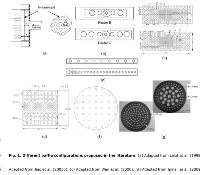
configurations proposed could be very different, even arbitrary, as illustrated in Fig. 1. The orifices
12
drilled in the plate could have identical or different diameters (usually small orifices at the centre of
13
baffle and big orifices on the edge), and be arranged in single line or in multiple lines. In any case, the
14
topology of the orifices' distribution, more specifically, the arrangement of the orifices on the plate
15
and their size distribution are either empirical or intuitive. To the best of our knowledge, neither
16
theoretical guidelines nor basic principles were proposed or established for the design and
17
optimization of the baffle configuration. This will result in two consequences since the equidistribution
18
effect of perforated baffle is generally restricted to a certain range of flow circuit geometry (eg.
19
number of parallel channels) and working condition (eg. inlet velocity). Firstly, the best topology
20
configuration of the perforated baffle can not be determined for one specific circuit geometry and
21
under certain working condition. Secondly, once the circuit geometry or working condition changes,
1
the equidistribution effect would probably be no longer in force. Then trial-and-error tests are
2
inevitable until finding a non-optimal but acceptable new configuration. As a result, the development
3
of a general method for the design and optimization of baffled fluid distributor is of great interests in
4
fields wherever the flow maldistribution problem exists.
5
In this study, a heuristic evolutionary algorithm (Luo et al., 2014) is proposed for the design and
6
shape optimization of baffled fluid distributor for uniform flow distribution. The algorithm is
7
CFD-based, and can be considered as a small extension in the general framework of Cellular
8
Automata (CA) (Wolfram, 2002). With this algorithm, we try to automatically evolve the size and
9
distribution of orifices on the perforated baffle in order to determine the optimal topology
10
configuration subject to each particular case. Compared to traditional arbitrary or empirical
11
propositions, this algorithm is more general, precise and flexible, and can be easily applied to
12
different distributor geometries and different working conditions.
13
We shall first present the heuristic algorithm with a general 2D case, appropriate for introducing basic
14
principles and for describing in detail each step of the algorithm. A numerical benchmark will then be
15
developed and optimization results will be presented. The influences of various design and
16
operational parameters will be analyzed and discussed. The theoretical basis for the extension of the
17
current algorithm to tackle 3D problem are also established. Finally, remarks and main conclusions
18
will be summarized.
19
Fig. 1. Different baffle configurations proposed in the literature. (a) Adapted from Lalot et al. (1999). (b) Adapted
20
from Jiao et al. (2003b). (c) Adapted from Wen et al. (2006). (d) Adapted from Ismail et al. (2009). (e) Adapted
from Wang et al. (2011). (f) Adapted from Krichnavaruk and Pavasant (2002). (g) Adapted from Maharaj et al.
1
(2007).
2
Table 1 Selected studies on fluid distributor with insertion of perforated baffle.
3
2. Heuristic evolutionary algorithm
4
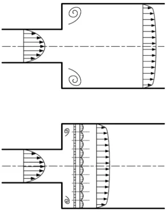
The basic idea of this study is to homogenize the velocity profile in the distributor by the insertion of
5
a perforated baffle instead of natural development, as shown in Fig. 2. The size and distribution of
6
orifices should be arranged in such a way that a regular velocity profile on the whole surface could be
7
achieved at the downstream of the baffle (before the inlets of parallel channels). To do that, we first
8
divide the baffle into numerous small sections, each section having an orifice in the middle. The
9
objective of the algorithm is to obtain identical fluid flux in every section by modulating the size of
10
every orifice. Locally uniform velocity profiles will then merge into a global regular one. We will
11
describe in detail in this section the basic principles and steps of this heuristic algorithm with a 2D
12
example. To simplify the numerical algorithm, we assume steady Newtonian fluid flow in this study.
13
Fig. 2. Schematic view of the effect of perforated baffle on the homogenization of velocity profile.
14
2.1. Introduction of notations
15
Fig. 3 shows a representative 2D baffled fluid distributor with single inlet tube (width w) and certain
16
amount of outlet channels (M) corresponding to the downstream equipment. The total inlet mass
17
flowrate equals to Q. A perforated baffle with thickness (e) is installed inside of the distributor. The
18
length of the baffle (L) is equal to the width of the distributor chamber and the location of baffle inside
19
the distributor (h/H) is a parameter subject to study. The baffle with length L is uniformly divided into
20
N control areas of same length l. Each control area i has one orifice of size di arranged in the middle,
1
and the flowrate passing through is qi. Then following relations could be derived based on geometric
2
considerations and mass conservation.
3
N
L
l =
(1)4
l
d
i i=
ε
(2)5
N
L
d
N i i N i i∑
∑
= ==
=
1 1ε
φ
(3)6
where εi is the local porosity in the ith control area, Φ the global porosity of the baffle.
7
Fig. 3. Representative example of a fluid distributor with insertion of perforated baffle.
8
The mean flowrate among orifices
q
can be calculated as:9
N
q
N
Q
q
N i i∑
==
=
1 (4)10
Note that the departure of qi from
q
depends on the location of the ith control area on the baffle and11
the size of the orifice di.
12
2.2. Basic principles
13
The objective of the evolutionary algorithm is to determine the optimal size distribution of orifices so
14
that the flowrate in every control area is identical.
15
l
q
l
q
l
q
i=
j=
(5)1
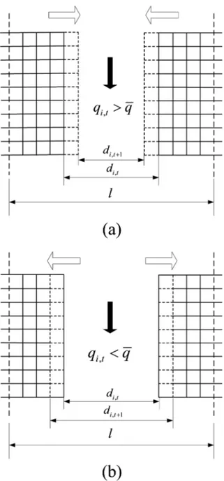
Practically, the diameter of each orifice di will be modulated by comparing qi and
q
, as explained in2
Fig. 4. More precisely, if the flowrate in the ith control area qi is larger than the mean value, then the
3
size of the orifice di should be reduced (Fig. 4a). Vice versa if qi is smaller than
q
, di should be4
enlarged so that it could receive higher amount of fluid flux (Fig. 4b). The variation of different di
5
according to the difference between qi and
q
repeats literally until the optimality criterion Eq. (5) is6
achieved. To realize this evolutionary procedure, a cellular automata based iterative program is
7
developed and will be described in next subsection.
8
Fig. 4. Basic principles of the optimization algorithm. (a) Reduction of the orifice. (b) Enlargement of the orifice.
9
Ideally, the increment or decrement of di from one optimization step to another should be as small as
10
possible (usually elemental cell length). However, that will by far lengthen the calculation time thus it
11
is not highly efficient. Therefore, we introduce a variation rule as presented in Eq. (6). Precisely from
12
t to t+1 step, the variation of di is proportional to the departure of qi,t from the mean value:
13
−
=
−
=
∆
+q
q
d
d
d
it t i t i t i, , 1 ,γ
1
, (6)14
γ is a relaxation factor to control the variation amplitude. Following this rule, the global porosity of the
15
baffle is kept constant during the optimization procedure:
16
0
1
1 , 1 ,=
−
=
−
=
∆
∑
∑
= =q
Q
N
q
q
d
N i t i N i itγ
γ
(7)17
t N i N i it t i N i it t
L
d
d
L
d
φ
φ
=
∆
+
=
=
∑
= +∑
=∑
= + 1 1 , , 1 , 1 1 (8)1
We also restrict that the boundary of the control area does not move during optimization (l is constant
2
and uniform) and that the boundary of orifice can not overstep the boundary of control area:
3
1
, ,=
l
≤
d
it t iε
(9)4
2.3. Implementation of optimization procedure
5
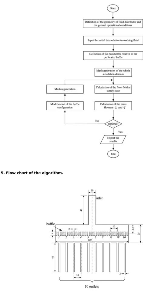
The optimization procedure is described in detail using the flow chart shown in Fig. 5.
6
1. Definition of the geometry of fluid distributor (width of inlet tube, number of channels,
7
etc.) as well as the general operational conditions such as the ambient temperature,
8
operational pressure, amount of heat exchange, etc.
9
2. Input the initial data relative to working fluid, such as the nature of fluid, the viscosity,
10
compressibility and density of the fluid (temperature and/or pressure dependent or
11
independent), gravity effect and viscous heating effect. The total inlet mass flowrate Q
12
should also be specified.
13
3. Definition of the parameters relative to the perforated baffle, such as the location and
14
thickness of baffle, number of control area N and the initial distribution of di.
15
4. Mesh generation of the whole simulation domain, thus the baffled fluid distributor.
16
Structured mesh is preferable for easy modification of fluid-solid interfaces.
17
5. Calculation of the exact flow field at steady state, by solving the Navier-Stokes equations.
1
6. Calculation of the mass flowrate qi passing through each control area and the mean value
2
of flowrate
q
; modification of the baffle configuration by comparing qi toq
, according3
to the rule presented in Eq. (6).
4
7. Regeneration of the mesh for updated simulation domain; recalculation of the exact flow
5
field.
6
8. Check the stable tolerance of the algorithm. If the tolerance is satisfied, then the heuristic
7
procedure is terminated. If not, the procedure goes back to Step 4 for recurrence. The
8
result is considered to be stable when the size variation at t step Δdi,t is smaller than
9
elemental cell size of the mesh. This also implies that the values of qi,t and
q
are very10
close.
11
9. Exportation of results, including the final configuration of perforated baffle, the flow
12
distribution uniformity among parallel outlet channels and the pressure drop of the
13
baffled distributor.
14
The flow maldistribution is quantified by two parameters: the relative flow rate deviation Di and the
15
maldistribution factor MF.16
f
f
f
D
i i−
=
(10)17
∑
=
−
−
=
M i if
f
f
M
1 21
1
MF
(11)18
where M stands for the number of parallel outlet channels. fi is the local mass flow rate in ith outlet
1
channel and
f
is the mean flowrate between parallel outlet channels. Uniform flow distribution is2
achieved when values of Di and MF approach 0.
3
M
f
M
Q
f
M i i∑
==
=
1 (12)4
Fig. 5. Flow chart of the algorithm.
5
2.4. Calculation of flow field by CFD method
6
One important step in the algorithm is the calculation of exact flow field in the baffled fluid distributor.
7
This generally involves solving Navier-Stokes equations by finite volume methods. The equation for
8
conservation of mass or continuity is:
9
( )
=
0
⋅
∇
+
∂
∂
u
t
ρ
ρ
(13)10
The momentum conservation equation is described by:
11
( )
u
(
uu
)
p
( )
g F
t
ρ
ρ
ρ
∂
+ ∇ ⋅
= −∇ + ∇ ⋅ ∏ +
+
∂
(14)12
where
u
is the velocity, p is the static pressure,ρ
g
andF
are the gravitational body force and13
external body forces,
∏
is the stress tensor which is given by:14
(
T)
2
3
u
u
uI
µ
∏ =
∇ + ∇
− ∇ ⋅
(15)15
where μ is the molecular viscosity, I is the unit tensor.
16
The energy equation is:
1
( )
E
(
u E p
(
)
)
(
T
)
:
u
Q
Ht
ρ
ρ
λ
ρ
∂
+ ∇ ⋅
+
= ∇ ⋅ ∇
+ ∏ ∇ +
∂
(16)2
where E is the internal energy,
λ
is the thermal conductivity, and QH includes the heat of chemical3
reaction, radiation and any other volumetric heat sources.
4
To predict turbulent flow pattern, additional turbulence models should be employed. It is worth noting
5
that besides the traditional CFD methods, new simulation techniques such as the Lattice Boltzmann
6
Method (LBM) can also be used in this regard for more complex fluid domains (Chen and Doolen, 1998;
7
Wang et al., 2010; 2014).
8
Having described the heuristic algorithm developed for uniform flow distribution, its effectiveness and
9
sensibility will be tested with an actual example in the next section.
10
3. Simulation and results
11
3.1. Numerical benchmark
12
Here a simple example of baffled fluid distributor restricted in a two-dimensional domain is
13
considered. Fig. 6 shows the schematic view of the case with main geometrical characteristics
14
indicated. The inlet tube is 10 mm (w) in width and 40 mm in length while the distributor chamber is
15
100 mm in width (L) and 25 mm in length (H). Ten parallel outlet channels (M=10) with identical
16
dimension of 2 mm in width and 40 mm in length are connected to the distributor chamber, spaced 10
17
mm from each other. Note that the inlet tube is located in the middle so that the whole geometry is
18
symmetrical.
19
In this study, the “sudden expansion configuration” of fluid distributor is selected as example because
1
it is the most compact but most difficult to realize the uniform flow distribution. However, the
2
proposed algorithm is not limited to this configuration but suitable for various geometries such as
3
distributors with 30° or 45° diffuser angle. The geometry of distributor may vary from case to case,
4
but the optimization procedure remains the same.
5
Fig. 6. Geometry and dimension of the numerical benchmark (unit: mm).
6
The 5 mm-thickness (e) perforated baffle is inserted at the middle of the distributor chamber
7
(h/H=0.5). The baffle is divided into 10 control areas (N=10), the length (l) of each being 10 mm. The
8
initial diameters of orifices are identical and equal to 2 mm (di,0=dj,0=2 mm), the global porosity (Φ)
9
being 20%. Note that the initial diameter distribution can be non-uniform, which will be discussed in
10
later subsections. The distribution of di evolves along with optimization steps while the global porosity
11
of the baffle is kept constant.
12
Liquid water is used as working fluid. The operation pressure is set at 101325 Pa. Simulations are
13
performed under steady state, isothermal condition without heat transfer. Gravity effect and viscous
14
heating are neglected for simplification. The physical properties of water used in the computation are
15
constant (density ρ=998.2 kg∙m-3; viscosity μ=1.003×10⁻³ kg∙m-1∙s-1).
16
Structured mesh is generated using software ICEMTM (version 12.1) to build up the geometry model.
17
Note that half of the real object is adopted for the purpose of lessening the computational burden
18
because of the symmetric feature of the simulation domain. Generally, one millimeter is divided into
19
ten segments to create square elemental cells. The influence of mesh density on the optimization
20
results is also tested and will be discussed later.
21
Navier-Stokes equations are resolved by a commercial code ANSYS FLUENTTM (version 12.1.4) to
1
calculate the flow field. Standard k-ε model is used to simulate the turbulent flow. For the
2
pressure-velocity coupling, COUPLED method is used. For discretization, standard method is chosen
3
for pressure and second-order upwind differentiation for momentum. Boundary conditions are set as
4
velocity inlet (1.0 m∙s-1) normal to the inlet boundary. Outlets are set to be static pressure boundary,
5
with pressure value being the same as ambient pressure. Adiabatic wall condition is applied and no
6
slip occurs at the wall. The solution is considered to be converged when (i) the mass flow-rate at each
7
outlet channel and the inlet static pressure are constant from one iteration to the next (less than
8
0.5% variation) and (ii) sums of the normalized residuals for control equations are all less than
9
1×10⁻⁶.
10
The optimization algorithm is written in MATLABTM. At each optimization step, it takes the computed
11
flow field results from FLUENTTM, performs calculations of the displacement according to the variation
12
rule and updates the coordinates of simulation domain. Then, it passes the data required to ICEMTM
13
to regenerate the mesh for the updated geometry.
14
3.2. Optimization results
15
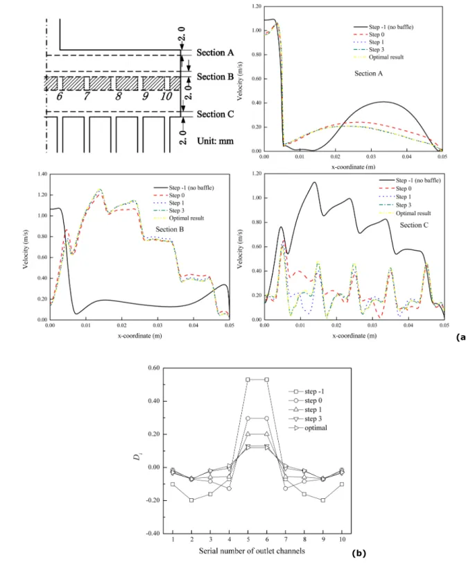
Fig. 7a shows the evolution of shape and flow field of different optimization steps at three sections of
16
the distributor. The locations of three sections are under the inlet tube, above the baffle and above the
17
parallel channels. Note that step -1 represents the empty distributor without baffle insertion as a
18
reference case while step 0 stands for the initial configuration of the baffle with identical size of
19
orifices. It can be seen that at step -1, the fluid tends to go preferentially into the channels that face
20
the inlet tube. The flow distribution among parallel outlet channels is obviously not uniform. The
21
insertion of uniformly perforated baffle (step 0) serves as an additional flow resistance (a second
1
header). Thus fluid flow is firstly distributed on the baffle plate before reaching the inlets of parallel
2
channels. The flow distribution is homogenized to some extent, but maldistribution still exists, as
3
indicated by the relative flowrate deviation curves shown on Fig. 7b. When the optimization algorithm
4
proceeds, the size distribution of orifices on the baffle evolves in such a way that the same fluid
5
flowrate passing through each orifice is approached. Finally, it reaches a relative steady-state, i.e. the
6
baffle configuration hardly changes as time step increases. In that case, each outlet channel has
7
almost the equal chance to receive the coming fluid, indicating a relatively homogenized flow
8
distribution.
9
Fig. 7. Shape and flow field evolution of different optimization steps at three sections (a); Relative flowrate
10
deviation of outlet channels for different optimization steps (b). N=10; M=10; Φ=20%; h/H=0.5; inlet velocity=1
11
m∙s-1.
12
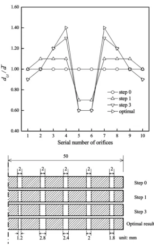
Examining the evolution of diameter distribution of orifices along with optimization time steps (Fig. 8),
13
we observe that the sizes of orifices at the centre (No. 5; 6) and at the edge (No. 1, 10) of the baffle
14
decrease while those at intermediate zone (No. 2-4; 7-9) increase. This observation differs from the
15
conventional proposition of a monotonously increasing size distribution from centre to the edge of the
16
baffle (eg. Jiao et al., 2003a; Wen and Li, 2004). In fact, the size reduction of central orifices is logical
17
since fluid should be guided toward the edge. As to the size reduction of peripheral orifices, it is a bit
18
counterintuitive owing to the backflow from the distributor walls (boundary effect). Anyway, the
19
optimal configuration of baffle is closely related to the geometry of fluid distributor.
20
Fig. 8. Evolution of size distribution of orifices on the baffle along with optimization steps. N=10; M=10; Φ=20%;
h/H=0.5; inlet velocity=1 m∙s-1.
1
Fig. 9 shows the evolution of flow maldistribution among parallel outlet channels as a function of
2
optimization time steps. It can be observed that the value of maldistribution factor MF reduces from
3
0.28 (empty distributor as reference) to 0.16 (initial configuration), and finally reaches 0.07
4
(optimized configuration). Although only several optimization steps are executed (7 steps for this
5
case, little change of flow distribution after the 4th step), the improvement of flow distribution
6
uniformity (optimized with respect to the initial configuration) is significant.
7
Fig. 9. Maldistribution factor (MF) and pressure drop (Δp) as a function of optimization steps. N=10; M=10;
8
Φ=20%; h/H=0.5; inlet velocity=1 m∙s-1.
9
The improved flow distribution uniformity is along with the increased pressure drop, as shown also in
10
Fig. 9. The value of pressure drop increases from 467 Pa (empty) to 676 Pa (initial configuration), and
11
finally reaches 730 Pa (optimized configuration). It can be observed that 79.5% of pressure drop
12
increase is caused by installing the baffle (step -1 to step 0). The pressure drop increase caused by
13
the optimization process is relatively small (20.5%). The heuristic algorithm realizes the optimal
14
allocation of pressure drop, which is the driving force to achieve flow equidistribution.
15
3.3. Sensibility analysis
16
Having presented the efficiency of proposed heuristic algorithm for uniform flow distribution, the
17
robustness of the algorithm regarding different influencing factors is now examined.
18
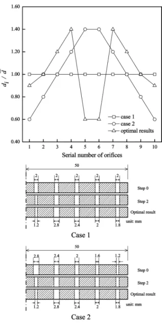
The choice of initial shape is usually important, especially for numerical optimization problems. In
19
order to investigate the sensibility of the algorithm to the choice of initial configuration, a comparative
20
test is carried out. This time a non-uniform size distribution of orifices is provided as initial
1
configuration of perforated baffle. All the boundary conditions and physical properties for fluid flow
2
are kept the same. It can be observed from Fig. 10 that by executing the optimization algorithm,
3
different initial configurations lead to a definite and unique optimized configuration. This justifies the
4
robustness of the proposed algorithm to the choice of the initial shape.
5
Fig. 10. Evolution of size distribution for different initial shapes.
6
Since in our algorithm the minimum size variation is defined as one cell of mesh, it is necessary to
7
assess the sensibility of the optimized results relative to mesh density. A comparative test regarding
8
the “resolution” of the simulated domain has been carried out. We have refined the mesh (20
9
segments instead of 10 for 1 mm) for the above distributor case, while keeping other numerical
10
parameters unchanged. Results on the improvement of flow distribution uniformity are presented in
11
Fig. 11. It may be observed that the flow distribution uniformity may be further improved when the
12
mesh density increases. This may be attributed to two reasons. On one hand, the calculation of flow
13
field is usually more accurate when more mesh nodes are available. On the other hand, the size
14
variation of orifices could be more precise with a smaller size of elemental cell. However, this further
15
improvement is at the cost of much longer computational time, since more computational time will be
16
consumed to calculate the flow field at each optimization step. For practical applications of the
17
algorithm in real engineering, the mesh density could be determined considering the fabrication
18
precisions and tolerance of maldistribution.
19
A “progressive refinement technique” may be considered to further improve the efficiency of our
20
algorithm. That is to use firstly coarse mesh and then progressively refine the flow domain in order to
21
reach the necessary density. This will be the subject of our future work.
1
Fig. 11. Influence of mesh density on the performance of optimization algorithm.
2
4. Effect of design parameters
3
In this section, the effects of design and operational parameters on the efficiency of the proposed
4
heuristic algorithm will be systematically evaluated. These parameters include the total inlet flowrate
5
(Q), the baffle location (h/H), the number of outlet tubes (M) and the global porosity (Φ).
6
4.1. Total inlet flowrate
7
Total inlet flowrate of a fluid distributor is one of the key operational parameters which is associated
8
with the throughput or capacity of processes. Meanwhile, it is also an influencing factor for flow
9
maldistribution since it is closed related to the flow patterns (laminar, transitional or turbulent) and
10
velocity profiles in the distributor., A parametric study is carried out by varying the inlet velocity from
11
0.1 m∙s-1 to 2.0 m∙s-1 in order to test the efficiency of our optimization algorithm within a wide range
12
of inlet flow rate. The corresponding Re number at inlet tube varies from 1000 to 20 000 while the
13
mean Re number at outlet channel changes from 100 to 2000.
14
Fig. 12a shows the evolution of flow distribution uniformity as a function of optimization time steps for
15
different values of inlet velocity. It can be easily observed that flow maldistribution augments with
16
increasing inlet velocity when no baffle is inserted in the distributor (step -1). This is mainly due to the
17
stronger inertial force at higher velocity so that the fluid enters the central outlet channels more
18
preferentially. The insertion of a uniformly perforated baffle (step 0) can reduce the maldistribution to
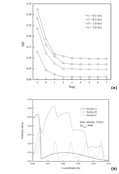
19
some extent, indicated by the reduction of maldistribution factor MF from 0.128 to 0.044 for 0.1 m∙s-1
inlet velocity and from 0.324 to 0.189 for 2.0 m∙s-1 inlet velocity. However, it is clear that the initial
1
configuration of baffle is not efficient enough to achieve uniform flow distribution under high inlet
2
flowrate conditions.
3
By applying the heuristic algorithm, the flow maldistribution can be further reduced. For the
4
optimized configurations, the MF value is 0.012 for 0.1 m∙s-1 inlet velocity and 0.096 for 2.0 m∙s-1
5
inlet velocity. The improvement of distribution uniformity is always significant with respect to the
6
initial configuration.
7
Fig. 12. Influence of inlet flowrate on the performance of optimization algorithm. N=10; M=10; Φ=20%; h/H=0.5
8
(a); Velocity of actual flow fields at three sections of the distributor. Inlet velocity=0.5 m∙s-1(b).
9
It should also be noted that the absolute distribution uniformity of the optimized configuration
10
decreases when total flowrate increases. This is mainly due to the higher inertial forces and locally
11
irregular and chaotic turbulences. Higher mesh density and more subtle size variation rule may be
12
useful to achieve a more uniform flow distribution under high flowrate conditions.
13
Fig. 12b shows the velocity of actual flow fields under 0.5 m∙s-1 inlet velocity at three sections of the
14
distributor. The flow fields are changed when the flow passes the perforated baffle. Five uniform
15
peaks correspond to five channels which make identical flow flux in each channel.
16
Fig. 13 shows that the total pressure drop in the distributor increases along with the increase of the
17
inlet velocity and higher pressure drop is inevitable to improve the distribution uniformity. As
18
mentioned above, the main pressure drop increase is caused by installing the baffle (Step -1 to Step
19
0), and the proportion caused by the optimization procedure is relatively small.
20
Fig. 13. Influence of inlet flowrate on the pressure drop in the baffled fluid distributor. N=10; M=10; Φ=20%;
1
h/H=0.5.
2
4.2. Location of the baffle
3
It is reported that location of the perforated baffle in the distributor chamber may influence the flow
4
distribution uniformity and the best location suggested is in the midway (Lalot et al., 1999). To verify
5
this influence, we have tested two additional cases with the baffle located at the upper-middle
6
(h/H=0.25) or at the bottom-middle (h/H=0.75) of the distributor chamber, to compare with the
7
midway case. Other numerical parameters are kept the same as the benchmark.
8
Fig. 14 shows the optimized flow distribution among parallel outlet channels for three different baffle
9
locations. It can be observed that the upper-middle case provides the most uniform optimized
10
distribution with maximum flowrate deviation Di less than 0.085. The optimized distribution of
11
bottom-middle case is relatively the least uniform, the maximum Di being 0.180. This implies that
12
under the circumstances of our example, longer distance between the baffle and parallel outlet
13
channels is beneficial for the remixing and redevelopment of flow profile at the downstream of the
14
perforated baffle. However, the shorter the distance between the inlet tube and the baffle, the higher
15
pressure drop will be generated, as shown in Fig. 15. The value of total pressure drop at optimized
16
configuration is 590.97 Pa, 730.46 Pa and 1213.57 Pa for the bottom-middle, midway and
17
upper-middle case, respectively. As a result, the best baffle location should be determined by a
18
trade-off between flow distribution uniformity and pressure drop increase.
19
Fig. 14. Relative flowrate deviation for optimized configurations with different baffle locations. N=10; M=10;
20
Φ=20%; inlet velocity=1 m∙s-1.
Fig. 15. Pressure drop as a function of optimization step, for different baffle locations. N=10; M=10; Φ=20%;
1
inlet velocity=1 m∙s-1.
2
4.3. Number of outlet channels M
3
The number of parallel outlet channels has certainly a great impact on the flow maldsitribution, since
4
it is by far more difficult to evenly divide one stream into dozens of small streams than into two or
5
three sub-streams. In order to test the efficiency of the heuristic algorithm within a wide range of
6
number of outlet channels (M), we studies two extra cases with M being 5 or 20. Other numerical
7
parameters are kept the same as the benchmark except that the distance between two neighboring
8
outlet channels is adjusted accordingly.
9
Fig. 16 shows the evolution of flow distribution uniformity as a function of optimization time steps for
10
different numbers of outlet channels. It can be observed that the larger the number of outlet channels,
11
the poorer the flow distribution uniformity will be. The value of maldistribution factor (MF) for the
12
empty distributor augments from 0.153 to 0.736 when M increases from 5 to 20. It is worth noting
13
that the optimized configuration obtained by the heuristic algorithm can always maintain the flow
14
maldistribution at a relatively low level, especially when the number of channels is large. It can also
15
be observed that the optimized distribution becomes relatively less uniform when M increases.
16
Fig. 16. Influence of number of outlet channels on the distribution uniformity. N=10; Φ=20%; h/H=0.5; inlet
17
velocity=1 m∙s-1.
18
A factor defined as the ratio of number of control areas to the number of outlet channels (N/M) is
19
introduced to explain these observations. Theoretically speaking, the insertion of perforated baffle
20
changes the “topological connectedness” from 1-M to 1-N-M. The heuristic optimization algorithm
1
could guarantee an equidistribution for the stage 1-N. For the stage N-M, it can be roughly analogized
2
as N empty distributors with topological connectedness of 1-M/N. The distribution uniformity in this
3
stage thus depends on the value of M/N. Specifically for the three cases tested, the distribution
4
uniformity is significantly improved compared to the reference case (1-M). Examining in more detail
5
the topological connectedness for each case, as schematically illustrated in Fig. 17, we notice that it
6
corresponds to 1-2 (bifurcation, M=20), 1-1 (straight, M=10) and 2-1 (merging, M=5) with internal
7
flow remixing, respectively. It will be easier to achieve equidistribution when fewer sub-streams
8
should be formed. Further discussion could be found in next subsection.
9
Fig. 17. Schematic view of the topological connectedness between the number of orifices and the number of
10
parallel outlet channels.
11
4.4. Global porosity Φ
12
A series of comparative tests were performed to study the effect of global porosity Φ on the
13
performance of the optimization algorithm. The control parameters for different cases are listed in
14
Table 2. It can be noticed that the tested global porosity (Φ) ranges from 10%, 20% to 40%. Higher
15
values of porosity may not be accepted since it may violate the constraint of Eq. (9) during the
16
evolution procedure (the boundary of the orifice may overstep the boundary of the control area). For
17
each value of global porosity, different numbers of control areas (N=10, 20, 40, 50) with
18
corresponding initial size of orifices are tested. Other parameters are kept identical, i.e. M=10,
19
h/H=0.5, inlet velocity at 1 m∙s-1.
20
Table 2 Control parameters for different tested cases.
Fig. 18. Influences of global porosity and number of orifices on the optimized flow distribution uniformity. M=10;
1
h/H=0.5; inlet velocity=1 m∙s-1.
2
Fig. 19. Influences of global porosity and number of orifices on the pressure drop increase. M=10; h/H=0.5; inlet
3
velocity=1 m∙s-1.
4
Fig. 18 presents the values of MF for optimized configurations of tested different cases. For a given
5
value of global porosity, larger number of orifices (N) is favorable for more uniform flow distribution.
6
This is coherent to the issue of “topological connectedness” discussed earlier. It seems that when the
7
number of orifices is large, the optimal distribution uniformity that can be achieved for different
8
porosities is very close. However, it should be noted that the absolute values of MF for these cases are
9
so small (less than 0.01) that they might be easily influenced by calculation errors or by the mesh
10
flaw.
11
Examining the pressure drop of the distributor for different cases as shown in Fig. 19, one may
12
observe that the increase of pressure drop due to the insertion of perforated baffle is inversely related
13
to the global porosity of the baffle. The higher the global porosity, the smaller the pressure drop
14
increase will be caused. This analysis indicates that higher global porosity with larger number of
15
orifices (while always keeping local porosity below 1) is beneficial to achieve both uniform flow
16
distribution and minimal pressure drop increase.
17
5. Extension to 3D
18
This problem will be addressed briefly in order to indicate how it can be handled, but without going
19
into details. In fact, the extension of current 2D algorithm to 3D geometry is astonishingly simple and
20
requires practically no rewriting. Let us merely illustrate the general cases of this point-to-surface
1
problem: a bundle of parallel channels evenly distributed on a rectangular or an oval surface to be
2
irrigated. Uniform flow distribution is required by a proper design of baffled fluid distributor, whose
3
inlet tube is located facing the centre of the surface.
4
The most delicate part of the exercise is actually to divide the surface (rectangular or oval) by control
5
volumes (instead of control areas for 2D cases), as shown in Fig. 20. Equations (1-3) can then be
6
easily rewritten by replacing linear parameters with surface parameters.
7
N
S
s =
(17)8
s
a
i i=
ε
(18)9
N
S
a
N i i N i i∑
∑
= ==
=
1 1ε
φ
(19)10
where S is the surface area of the baffle, s the surface area of the control volume and ai the size of the
11
orifice in ith control volume. The basic principles of the optimization algorithm and evolution rules for
12
the 3D case are:
13
s
q
s
q
s
q
i=
j=
(20)14
−
=
−
=
∆
+q
q
a
a
a
it t i t i t i, , 1 ,γ
1
, (21)15
It can be easily verified that the global porosity does not change along with the optimization steps.
16
Implementing the same optimization procedure as for 2D cases, uniform flow distribution may be
17
expected using our heuristic algorithm. Of course, more computational time is also needed for the
1
calculation of flow field at each optimization step by CFD code.
2
Note that the shape of control volumes may be rectangular, regular hexagon or those may uniformly
3
pave the entire baffle surface. As to the orifices, the simplest shape is circular or square since the area
4
variation at each optimization step can be realized by modulating single variable (diameter or side
5
length). Of course, other shapes are also realizable regarding different geometries, with the
6
constraint that the boundary of orifice does not overstep the boundary of the control volume during
7
optimization.
8
Fig. 20. Division of a baffle surface by numerous control volumes for 3D application.
9
6. Discussion
10
In the current algorithm, uniform and identical value of pressure is assigned as boundary condition
11
for outlet channels. This approximation is appropriate for the shape optimization of inlet fluid
12
distributor as an individual device. However, in compact systems where inlet distributor, parallel
13
channels for unit process operation and outlet collector are highly integrated and closely connected,
14
the configuration of the downstream collector may have a noticeable impact on the upstream flow
15
distribution uniformity between parallel channels. In this case, the algorithm should be modified so
16
that the simulation domain covers the entire geometry from the single inlet to the single outlet. The
17
optimization rule should be updated accordingly as well.
18
Basic constraints for the proposed algorithm are that the control areas (volumes) are evenly divided
19
and that the boundary of orifices can not overstep the boundary of control areas during optimization
20
steps (local porosity less than 1). These constraints are useful and necessary to guarantee a uniform
1
flow distribution among parallel channels evenly spaced between one another on a line or on a surface.
2
However, when non-uniform but controlled flow distribution is required or unevenly spaced parallel
3
channels are involved in certain operational equipment, these constraints should be modified
4
accordingly. In that case, an additional degree of freedom may be added, i.e. the lengths of control
5
area li (surface areas ai for 3D application) can be locally varied (li≠lj; li,t≠li,t+1) corresponding to
6
specified optimization criterion, while keeping the global porosity constant during optimization.
7
The baffle configuration optimization with our algorithm will surely cause a certain increase of
8
pressure drop in the distributor. However, this pressure drop increase which depends on the
9
configuration of baffle could be relatively small (higher porosity; smaller thickness but within the limit
10
of mechanical deformation). Moreover, this increase can be compensated by the reduced pressure
11
drop of downstream equipment owing to more uniform flow distribution.
12
It should be noted that the efficiency of the heuristic algorithm depends largely on the precision of the
13
transport phenomena simulation. The more realistic the simulated flow, the more satisfactory results
14
may be achieved. When more complex flows such as varied fluid composition or more complicated
15
situations such as fouling or channel blockage are involved, the selection of adaptive and reliable
16
numerical models is very important. However, the heuristic algorithm is somewhat independent to the
17
CFD codes used.
18
7. Conclusion and prospects
19
This paper presents a CFD-based, heuristic evolutionary algorithm for shape design and optimization
20
of baffled fluid distributor. In this algorithm, the baffle surface is firstly divided with numerous
21
identical control areas (volumes), each control area having an orifice in the middle. Under the
1
constraint of constant global porosity of the baffle, the algorithm adjusts the size distribution of
2
orifices so as to approach identical mass flowrate passing through every control area. An automatic
3
program is processed iteratively so that the baffle configuration evolves toward the optimized shape,
4
providing a uniform flow distribution among parallel outlet channels.
5
Compared to traditional arbitrary or empirical propositions, the advantages of our optimization
6
algorithm lie in two main aspects. On the one hand, it leads to an optimal baffle configuration for a
7
given distributor geometry under certain working condition. On the other hand, it may be easily
8
applied to different flow circuit geometries (eg. different numbers of outlet channels) and different
9
working conditions (eg. different total flowrate). In this sense, this algorithm is robust, effective,
10
general and flexible.
11
The examples presented in this study deal with single phase flow. The extension of the proposed
12
algorithm for multi-phase flow maldistribution problem is interesting but challenging. This is one
13
direction of our future work and some guidelines may be followed based on the recent works of
14
Schouten’s group (Al-Rawashdeh et al., 2012a, 2012b, 2012c, 2014).
15
It should be noted that higher global performances of devices (in terms of higher thermal efficiency,
16
presence of less hot spots, enhanced mixing, controlled reaction, etc.) for different applications may
17
need different optimal criterion (Mies et al., 2007; Al-Rawashdeh et al., 2013). The development a
18
pertinent performance criterion for special unit operation, and the experimental validation of the
19
optimization algorithm for an actual application are the directions of our ongoing work.
20
Acknowledgement
1
This work is partially financed by the French CNRS within the project AAP-Energie 2012 of INSIS. One
2
of the authors M. Min WEI would like to thank the “Région Pays de la Loire” for its partial financial
3
support to his PhD study.
4
Notations
1
a size of the orifice in 3D m2
d diameter of orifices m
D flow rate ratio -
e thickness of the perforated baffle m
E internal energy per unit mass J kg-1
f mass flowrate in outlet channels kg s-1
f
mean mass flowrate among outlet channels kg s-1F external body force kg m s-2
g gravitational acceleration m s-2
h length between inlet and baffle m
H length of distributor m
I unit tensor -
l length of control area m
L length of baffle m
M number of outlet channels -
MF maldistribution factor -
N number of control areas -
p pressure Pa
q mass flowrate through orifices kg s-1
Q total inlet mass flowrate kg s-1
QH external heat transfer flux J kg-1 s-1
Re Reynolds number -
s surface area of control volume in 3D m2
S surface area of baffle in 3D m2
t time step -
T temperature K
u velocity m s-1
w width of inlet tube m
1
Greek symbols2
γ
relaxation factor - ε local porosity -λ
thermal conductivity W m-1 K-1 µ viscosity kg m-1 s-1∏
stress tensor - ρ density kg m-3 Φ global porosity -3
Subscriptsi, j orifice and channel index
References
1
Ajmera, S.K., Delattre, C., Schmidt, M.A., Jensen, K.F., 2002. Microfabricated differential reactor for
2
heterogeneous gas phase catalyst testing. Journal of catalysis 209(2), 401-412.
3
Al-Rawashdeh, M., Fluitsma, L.J.M., Nijhuis, T.A., Rebrov, E.V., Hessel, V., Schouten, J.C., 2012a.
4
Design criteria for a barrier-based gas-liquid flow distributor for parallel microchannels. Chemical
5
Engineering Journal 181-182, 549-556.
6
Al-Rawashdeh, M., Nijhuis, X., Rebrov, E.V., Hessel, V., Schouten, J.C., 2012b. Design methodology
7
for barrier-based two phase flow distributor. AIChE Journal 58(11), 3482-3493.
8
Al-Rawashdeh, M., Yu, F., Nijhuis, T.A., Rebrov, E.V., Hessel, V., Schouten, J.C., 2012c. Numbered-up
9
gas-liquid micro/millichannels reactor with modular flow distributor. Chemical Engineering Journal
10
207-208, 645-655.
11
Al-Rawashdeh, M., Yu, F., Patil, N.G., Nijhuis, T.A., Hessel, V., Schouten, J.C., Rebrov, E.V.,
12
2014.Designing flow and temperature uniformities in parallel microchannels reactor.AIChE Journal
13
60(5), 1941-1952.
14
Al-Rawashdeh, M., Zalucky, J., Muller, C., Nijhuis, T.A., Hessel, V., Schouten, J.C.,
15
2013.Phenylacetylene hydrogenation over [Rh(NBD)(PPh3)2]BF4 Catalyst in a numbered-up
16
microchannels reactor. Industria& Engineering Chemistry Research 52(33), 11516-11526.
17
Barber, R.W., Emerson, D.R., 2008. Optimal design of microfluidic networks using biologically inspired
18
principles. Microfluidics and Nanofluidics 4(3), 179-191.
19
Chein, R., Chen, J., 2009. Numerical study of the inlet/outlet arrangement effect on microchannel
1
heat sink performance. International Journal of Thermal Sciences 48(8), 1627-1638.
2
Chen, S., Doolen, G.D., 1998. Lattice Boltzmann method for fluid flows. Annual review of fluid
3
mechanics 30(1), 329-364.
4
Chen, Y., Zhang, C., Shi, M., Yang, Y., 2010. Thermal and hydrodynamic characteristics of constructal
5
tree‐shaped minichannel heat sink. AIChE Journal 56(8), 2018-2029.
6
Commenge, J., Falk, L., Corriou, J., Matlosz, M., 2002. Optimal design for flow uniformity in
7
microchannel reactors. AIChE Journal 48(2), 345-358.
8
Commenge, J., Saber, M., Falk, L., 2011. Methodology for multi-scale design of isothermal laminar
9
flow networks. Chemical Engineering Journal 173(2), 541-551.
10
Dang, T., Teng, J.-T., 2011. Comparisons of the heat transfer and pressure drop of the microchannel
11
and minichannel heat exchangers. Heat and mass transfer 47(10), 1311-1322.
12
Fan, Y., Boichot, R., Goldin, T., Luo, L., 2008a. Flow distribution property of the constructal distributor
13
and heat transfer intensification in a mini heat exchanger. AIChE Journal 54(11), 2796-2808.
14
Fan, Z., Zhou, X., Luo, L., Yuan, W., 2008b. Experimental investigation of the flow distribution of a
15
2-dimensional constructal distributor. Experimental Thermal and Fluid Science 33(1), 77-83.
16
Gheorghiu, S., Kjelstrup, S., Pfeifer, P., Coppens, M.-O., 2005. Is the lung an optimal gas exchanger?
17
Fractals in biology and medicine. Springer.
18
Guo, X., Fan, Y., Luo, L., 2013. Mixing performance assessment of a multi-channel mini heat
19
exchanger reactor with arborescent distributor and collector. Chemical Engineering Journal 227,
1
116-127.
2
Idelchik I.E., 1991. Fluid Dynamics of Industrial Equipment: Flow distribution design methods.
3
Hemisphere.
4
Jiao, A., Li, Y., Chen, C., Zhang, R., 2003a. Experimental investigation on fluid flow maldistribution in
5
plate-fin heat exchangers. Heat Transfer Engineering 24(4), 25-31.
6
Jiao, A., Zhang, R., Jeong, S.K., 2003b. Experimental investigation of header configuration on flow
7
maldistribution in plate-fin heat exchanger. Applied thermal engineering 23(10), 1235-1246.
8
Krichnavaruk, S., Pavasant, P., 2002. Analysis of gas–liquid mass transfer in an airlift contactor with
9
perforated plates. Chemical Engineering Journal 89(1), 203-211.
10
Kumaran, R.M., Kumaraguruparan, G., Sornakumar, T., 2013. Experimental and numerical studies of
11
header design and inlet/outlet configurations on flow mal-distribution in parallel micro-channels.
12
Applied Thermal Engineering 58, 205-216.
13
Lalot, S., Florent, P., Lang, S., Bergles, A., 1999. Flow maldistribution in heat exchangers. Applied
14
thermal engineering 19(8), 847-863.
15
Liu, H., Li, P., 2013. Maintaining equal operating conditions for all cells in a fuel cell stack using an
16
external flow distributor. International Journal of Hydrogen Energy 38(9), 3757-3766.
17
Luo, L., Fan, Y., Wei, M., Flamant, G., 2014. Procédé de détermination de caractéristiques d'orifices à
18
ménager à travers une plaque et programme correspondant, Brevet français (French Patent)
19
PN000441.
1
Luo, L., Fan, Y., Zhang, W., Yuan, X., Midoux, N., 2007. Integration of constructal distributors to a mini
2
crossflow heat exchanger and their assembly configuration optimization. Chemical engineering
3
science 62(13), 3605-3619.
4
Luo, L., Fan, Z., Le Gall, H., Zhou, X., Yuan, W., 2008. Experimental study of constructal distributor for
5
flow equidistribution in a mini crossflow heat exchanger (MCHE). Chemical Engineering and
6
Processing: Process Intensification 47(2), 229-236.
7
Maharaj, L., Pocock, J., Loveday, B., 2007. The effect of distributor configuration on the
8
hydrodynamics of the teetered bed separator. Minerals Engineering 20(11), 1089-1098.
9
Manikanda Kumaran, R., Kumaraguruparan, G., Sornakumar, T., 2013. Experimental and Numerical
10
Studies of Header Design and Inlet/Outlet Configurations on Flow Mal-distribution in Parallel
11
Micro-channels. Applied Thermal Engineering 58(1-2), 205-216.
12
Midoux, N., Tondeur, D., 2014. The theory of parallel channels manifolds (Ladder networks) revisited
13
part 1: Discrete mesoscopic modelling. The Canadian Journal of Chemical Engineering 92(10),
14
1798-1821.
15
Midoux, N., Tondeur, D., 2014. The theory of parallel channels manifolds (Ladder networks) revisited
16
part 2. The Canadian Journal of Chemical Engineering, in press.
17
Mies, M.J.M., Rebrov, E.V., Deutz, L., Kleijn, C.R., De Croon, M.H.J.M., Schouten, J.C., 2007.
18
Experimental validation of the performance of a microreactor for the high-throughput screening of