HAL Id: hal-01413037
https://hal.inria.fr/hal-01413037
Submitted on 15 Dec 2016HAL is a multi-disciplinary open access archive for the deposit and dissemination of sci-entific research documents, whether they are pub-lished or not. The documents may come from teaching and research institutions in France or abroad, or from public or private research centers.
L’archive ouverte pluridisciplinaire HAL, est destinée au dépôt et à la diffusion de documents scientifiques de niveau recherche, publiés ou non, émanant des établissements d’enseignement et de recherche français ou étrangers, des laboratoires publics ou privés.
with rotational inertia
Francesco Bonaldi, Giuseppe Geymonat, Françoise Krasucki, Marina Vidrascu
To cite this version:
Francesco Bonaldi, Giuseppe Geymonat, Françoise Krasucki, Marina Vidrascu. Mathematical and numerical modeling of plate dynamics with rotational inertia. Journal of Numerical Mathematics, De Gruyter, 2017, 26 (1), pp.1 - 20. �10.1515/jnma-2016-1020�. �hal-01413037�
dynamics with rotational inertia
Francesco Bonaldi, Giuseppe Geymonat, Françoise Krasucki and
Marina Vidrascu
Abstract. We give a presentation of the mathematical and numerical treatment of plate dynamics problems including rotational inertia. The presence of rotational inertia in the equation of motion makes the study of such problems interesting. We employ HCT fi-nite elements for space discretization and the Newmark method for time discretization in FreeFEM++, and test such methods in some significant cases: a circular plate clamped all over its lateral surface, a rectangular plate simply supported all over its lateral surface, and an L-shaped clamped plate.
Keywords. Plates, Kirchhoff-Love, Rotational inertia, FreeFEM, HCT, Newmark. 2010 Mathematics Subject Classification. 74K20, 65M60, 35Q74.
General notation
We denote by Ω Ă R2 a two-dimensional domain with smooth boundary Γ; Γ0 Ă Γ is a measurable subset of Γ, with strictly positive length measure, and Γ1 “ ΓzΓ0. The outer unit normal and tangent vector fields on Γ are denoted, respectively, by n “ pn1, n2q and τ “ p´n2, n1q. For ψ a real-valued field de-fined on Ω, Bnψ “ ∇ψ ¨ n and Bτψ “ ∇ψ ¨ τ denote its normal and tangential derivatives on Γ. The space dependence of a field is left tacit, unless noted other-wise. The time derivative of a real- or vector-valued field ϕ is denoted by 9ϕ, of a function Φ taking values in a Hilbert space by dΦdt. Finally, Symp2q denotes the space of symmetric second-order tensors in R2.
Introduction
In [6] the equations of plate models for magneto-electro-thermo-elastic sensors and actuators have been deduced by an asymptotic development with respect to
This work has been partially supported by the French Agence Nationale de la Recherche (ANR) under grant ARAMIS (Projet «Blanc», N. ANR 12 BS01-0021) (Analysis of Robust Asymptotic Methods in Numerical Simulation in Mechanics).
the thickness 2e ą 0 of the plate. A peculiar feature of the different models concerns the flexural problem, governing the evolution of the transversal dis-placement w of the plate, which occupies the closure of the three-dimensional domain Ω ˆ p´e, eq in its reference configuration and whose kinematics is of Kirchhoff-Love type. This problem is uncoupled from the membrane problem, it takes into account an inertia effect involving the mean curvature of the de-formed middle surface, referred to as rotational inertia, and the only influence of magneto-electro-thermo-elastic behavior of the material appears in the coeffi-cients A “ pAαβστq of the (symmetric) moment tensor Mptq “ pMαβptqq “ ´2e33A∇∇wptq, p∇∇wptqqαβ “ Bαβwptq (let us point out that the fourth-order tensor A “ pAαβστq is symmetric and strongly elliptic). The transverse displacement w of the plate is solution of the following evolution equation:
2eρ :w ´2e 3
3 ρ 4 :w ´ div div M “ f ` div m in Ω ˆ p0, T q, (1) equipped with initial conditions
wp0q “ w0, 9wp0q “ w1 in Ω (2) and with suitable boundary conditions, where ρ ą 0 is the mass density of the plate, supposed to be homogeneous. If one supposes, for the sake of simplic-ity, that the three-dimensional body is subjected to time-dependent volume forces p0, 0, F ptqq and surface loads pG1˘ptq, G˘2ptq, 0q on the upper and lower faces Ωˆ t˘eu, then the source terms in the right-hand side of (1) have the follow-ing expressions
f ptq “ ż`e
´e
F ptq dx3, mαptq “ epG`αptq ´ Gα´ptqq, α P t1, 2u. (3)
The term accounting for rotational inertia in (1) is ´2e33ρ4 :w, and it derives from the expression of the volume kinetic energy kptq for Kirchhoff-Love plates subjected to pure bending:
kptq “ 1 2 ˆ 2eρ 9w2`2e 3 3 ρ|∇ 9w| 2 ˙ .
The reason for the word rotational is that the quantity |∇w| gives a measure of the rotation of the material fibers orthogonal to the middle surface of the plate, which remain straight and perpendicular to this surface after deformation in Kirchhoff-Love kinematics.
The influence of rotational inertia on the lateral vibrations of linearly elastic bars was considered by Lord Rayleigh [20], sect. 186; the extension of this analysis to the flexural motion of isotropic elastic plates was carried out for the first time in 1951 in a seminal paper by R. D. Mindlin [16] where also the effect of transverse shear deformation is taken into account. Later on, an evolution model for plates with rotational inertia was deduced by A. Raoult [18] using the asymptotic expan-sion method. The influence of such effects has also been considered in the case of flexural motion of large amplitude. Analogously to the case of beams, where it can be worth to account for rotational inertia of the cross section in case the slen-dernessof the beam (i.e., the ratio of the cross section diameter to the length of the beam) is lower than one, but not very close to zero, in our case rotational inertia of the material fibers orthogonal to the middle surface may be important if the plate thinness(i.e., the ratio of the thickness to the diameter of the plate) is lower than one, but not very close to zero. In the following, to point out the influence of the thickness parameter, we carry out our analysis on equation (1) divided by 2e.
Our goal, after providing a result of well-posedness for the problem, is to test a numerical method involving C1elements for what concerns space discretization and Newmark’s midpoint method concerning time discretization. The presence of the rotational inertia requires an appropriate choice of the functional spaces, presented in sect. 1, where we sketch the proof of the well-posedness using the Faedo-Galerkin method. In sect. 2 we perform, in the appropriate Sobolev spaces, the error analysis of a finite element spatial discretization and of a Newmark-type discrete time approximation. Our choice allows the application of the methods developed for linear second-order evolution equations. Based on a continuous-time Galerkin method (see e.g. [2] or [11]) we can infer optimal error estimates, and then couple with the error estimates for the time discretization of Newmark type (see e.g. [19]). Note that a conforming space discretization for plates requires C1elements; we choose HCT elements (see e.g. [7]). This theoretical numerical analysis is complemented with numerical tests performed with FreeFEM++.
Let us remark that the choice of C1elements is not very common in practice, as these elements are rather expensive. Mixed and hybrid plate elements were exten-sively studied. Among the elements widely used in the engineering community we can mention the DKT triangle [3]. For a general review of plate elements see for example [5], [14] and references therein. We can also mention the more modern hybrid high-order methods [8, 9]: they will be studied in a forthcoming paper.
1
Existence and uniqueness
We start by rewriting (1) as ρ :w ´e 2 3ρ4 :w ´ e23div div A∇∇w “ 1
2epf ` div mq. (4) The weak formulation of the problem depends on boundary conditions. For this, we first define the pivot space
H “ tu P H1pΩq : u “ 0 on Γ0u (5) and the bilinear form b : H ˆ H Ñ R given by
bpu, vq “ ż Ω ˆ ρuv `e 2 3ρ∇u ¨ ∇v ˙ dΩ, @u, v P H. (6)
Notice that bp¨, ¨q defines a scalar product in H whose associated norm | ¨ |b is equivalent to the usual Sobolev norm.
Let V be a Hilbert-Sobolev space such that
piq V Ď H2pΩq X H,
piiq the embedding V ãÑ H is compact.
Thanks to piq, we can endow V with the Hessian L2-norm given by
}v} “ ˆ ż Ω ∇∇v : ∇∇v dΩ ˙1{2 . (7)
Let us define the bilinear form a : V ˆ V Ñ R by apu, vq “ e 2 3 ż Ω A∇∇u : ∇∇v dΩ, @u, v P V. (8)
By the symmetry and ellipticity properties of A, there exist two positive constants A´and A`such that, for all x P Ω,
A´|U|2
ď AU :U ď A`|U|2, @U P Symp2q.
Hence, ap¨, ¨q is symmetric and V-elliptic: apv, vq ě e32A´}v}2for any v P V . In the numerical examples, we consider essentially the following situations:
pBCq1: $ ’ & ’ % 2e3 3 ρ Bnw ` div M ¨ n ` B: τpMn ¨ τ q “ ´m ¨ n on Γ1ˆ p0, T q, Mn ¨ n “ 0 on Γ1ˆ p0, T q, w “ 0, Bnw “ 0 on Γ0ˆ p0, T q,
pBCq2: $ ’ & ’ % 2e3 3 ρ Bnw ` div M ¨ n ` B: τpMn ¨ τ q “ ´m ¨ n on Γ1ˆ p0, T q, Mn ¨ n “ 0 on BΩ ˆ p0, T q, w “ 0 on Γ0ˆ p0, T q.
Boundary conditions pBCq1refer to a plate clamped on Γ0; in this case we choose V “ V1“ tu P H2pΩq : u “ Bnu “ 0 on Γ0u. (9) Boundary conditions pBCq2feature a plate simply supported on Γ0, in which case we choose
V “ V2“ tu P H2pΩq : u “ 0 on Γ0u “ H2pΩq X H. (10) In both cases, under the general hypothesis of anisotropic linearly elastic behavior, the weak formulation of the problem has the following aspect:
$ ’ ’ ’ ’ ’ ’ ’ ’ & ’ ’ ’ ’ ’ ’ ’ ’ %
For any fixed t P p0, T q, find wptq P V such that ż Ω ˆ ρ :wptqv `e 2 3ρ∇ :wptq ¨ ∇v ` e2 3A∇∇wptq : ∇∇v ˙ dΩ “ 1 2e ż Ω pf ptqv ´ mptq ¨ ∇vq dΩ,
for all v P V, with initial conditions wp0q “ w0, 9wp0q “ w1,
(11)
where V “ V1or V “ V2.
Remark 1.1. Notice that, by taking volume and surface loads constant in space in (3), we have f ptq “ 2eF ptq and mαptq “ epGα`ptq´Gα´ptqq, so that the right-hand sides of (4) and of (11) are independent of the thickness.
In order to show that problem (11) is well-posed, we identify the time-dependent linear form on H Ltpvq “ 1 2e ż Ω pf ptqv ´ mptq ¨ ∇vq dΩ,
with the scalar product of an element F ptq P H (for 0 ă t ă T ) with v P H. This can be accomplished via the following problem:
Find F ptq P H such that bpF ptq, vq “ Ltpvq, @v P H.
(12)
Provided f ptq P L2pΩq and mptq P L2pΩq for 0 ă t ă T , problem (12) is well-posed by the Lax-Milgram Lemma. As for problem (11), we assume
f P L2p0, T ; L2pΩqq and m P L2p0, T ; L2pΩqq, so that F P L2p0, T ; Hq; the formulation of the problem reads then:
Givenw0P V , w1P H and F P L2p0, T ; Hq, find a function w such that w P C0pr0, T s; V q X C1pr0, T s; Hq and, for all v P V,
d2 dt2bpwptq, vq ` apwptq, vq “ bpF ptq, vq, wp0q “ w0, dw dtp0q “ w1. (13)
Theorem 1.2. Let T ą 0 be fixed, w0P V , w1P H and F P L2p0, T ; Hq.
(i) There exists a unique function w P C0pr0, T s; V q X C1pr0, T s; Hq satisfying (13).
(ii) For all t P r0, T s, the function w satisfies the following energy equation:
| 9wptq|2b` apwptq, wptqq “ |w1|2b` apwp0q, wp0qq ` 2 żt
0
bpF psq, 9wpsqq ds.
(iii) There exists a constant c “ cpΩ, Aq such that }w}C0pr0,T s;V q` }w}C1pr0,T s;Hqď ? T e cpΩ, Aq ´ }w0}`|w1|b`}F }L2p0,T ;Hq ¯ .
For a proof of statements (i) and (iii) of Theorem 1.2, of which we present hereinafter some essential parts, see e.g. [1] and [19] (see also [10], for a general treatment of evolution equations); the proof of statement (ii) can be found in [15, Chap. 3, Sect. 8] where a very general situation is considered. The uniqueness of the solution is proven in a standard way. With the choice (9) or (10) of the space V , and (5) for the space H, endowed with scalar products (8) and (6) respectively, the Faedo-Galerkin approximation method can be used. The compactness of the embedding V ãÑ H implies that there exists an increasing sequence of eigenvalues 0 ă λ1 ď λ2 ď . . . ď λi ď . . . and a Hilbert basis tgiu, orthonormal in H and orthogonal in V , of associated eigenvectors verifying
@v P V, apgi, vq “ λibpgi, vq
(see e.g. [?]). As for existence, the subspace Vm of V generated by the first m eigenvectors g1, . . . , gmis introduced; let wm: t P r0, T s ÞÑ wmptq P Vmbe
solu-tion to the following (well-posed) second-order system of differential equasolu-tions: @vmP Vm, d2 dt2bpwmptq, vq ` apwmptq, vq “ bpF ptq, vq, (14) wmp0q “ w0,m“ m ÿ i“1 bpw0, giqgi, dwm dt p0q “ w1,m“ m ÿ i“1 bpw1, giqgi. (15)
One can show that twmumPN is a Cauchy sequence in spaces C0pr0, T s; V q and C1pr0, T s; Hq and thus it converges to a function w in such spaces. Finally, by a density argument, it is proven that w is solution to (13).
2
Numerical analysis
2.1 Semi-discrete problem
Let Vh Ă V denote a subspace of V of dimension I “ Iphq and consider the following semi-discrete problem: given w0,h P Vhandw1,h P Vh, find the solu-tionwh: t P r0, T s ÞÑ whptq P Vhto the following system of ordinary differential equations: @vhP Vh, d2 dt2bpwhptq, vhq ` apwhptq, vhq “ bpF ptq, vhq, whp0q “ w0,h, dwh dt p0q “ w1,h. (16)
We now introduce a basis tϕiu1ďiďI of Vhand denote the time-dependent com-ponents of wh in this basis by ξjptq, j “ 1, . . . , I. Analogously, we denote the components in the same basis of w0,h and w1,h respectively by ξ0,j and ξ1,j. Fi-nally, we set χhjptq “ bpF ptq, ϕjq. Then (16) reads
#
Mhξptq ` K: hξptq “ χhptq, ξp0q “ ξ0, ξp0q “ ξ9 1,
(17)
with self-explanatory notation. Matrices Mh and Kh are respectively the mass matrixand the stiffness matrix. Their coefficients are
pMhqij “ bpϕi, ϕjq and pKhqij “ apϕi, ϕjq, 1 ď i, j ď I. (18) In the following, we drop the index h when there is no ambiguity.
Remark 2.1. The choice of the scalar product (6) in H ensures that M is positive definite.
Problem (17) is the semi-discrete counterpart of (13). Under certain in-time regu-larity hypotheses on w and adapting the arguments of [2], [11], it is possible to give an estimate of the error whptq ´ wptq. For this, we introduce the elliptic projection operator Πh, a linear and continuous operator mapping u P V onto Πhu P Vh defined by
@vhP Vh, apΠhu ´ u, vhq “ 0. We have the following results.
Theorem 2.2. Let T ą 0 be fixed and assume that the solution w of (13) verifies w P C2
pr0, T s; V q. Then there exists a constant C “ CpAq independent of h such that, for anyt P r0, T s,
}whptq ´ wptq} ` ˇ ˇ ˇ ˇ dwh dt ptq ´ dw dtptq ˇ ˇ ˇ ˇ b ď 1 eCpAq ˆ }w0,h´ Πhw0} ` |w1,h´ Πhw1|b` }pI ´ Πhqwptq} ` ˇ ˇ ˇ ˇpI ´ Πhq dw dtptq ˇ ˇ ˇ ˇ b ` żt 0 ˇ ˇ ˇ ˇpI ´ Πhq d2w dt2psq ˇ ˇ ˇ ˇ b ds ˙ .
Theorem 2.3. Under the assumptions of Theorem 2.2 let the following approxima-tion hypotheses be satisfied:
@v P V, lim hÑ0vhinfPVh }v ´ vh} “ 0, (19) lim hÑ0}w0,h´ w0} “ 0, (20) lim hÑ0|w1,h´ w1|b “ 0; (21) then @t P r0, T s, lim hÑ0 ˆ }whptq ´ wptq} ` ˇ ˇ ˇ ˇ dwh dt ptq ´ dw dtptq ˇ ˇ ˇ ˇ b ˙ “ 0.
This convergence result can actually be improved; under the hypotheses of Theo-rem (1.2),
lim
hÑ0wh“ w in C 0
2.2 Time discretization: Newmark’s midpoint method
A typical time discretization method widely used for differential systems of the form (17) is the Newmark method (see, e.g., [12]). In particular, we will use a midpointapproximation.
Let N P N; we introduce a time-step ∆t “ NT and a uniform mesh of the interval r0, T s defined by nodes tn “ n∆t, 0 ď n ď N . We want to compute an approximation ´ ξn, 9ξn ¯ of the pair ´ ξptnq, 9ξptnq ¯ . The discretization of (17) based on Newmark’s midpoint method can be rewritten as
$ ’ & ’ % ˆ M `∆t 2 4 K ˙ ξn`12 “ Mξn`∆t 2M 9ξ n `∆t 2 4 χ n`12, 0 ď n ď N ´ 1, ξ0“ ξ0, ξ90“ ξ1 (22) with ξn`12 “ 1 2`ξn`1` ξ n˘ and χn`12 “ 1 2pχptn`1q ` χptnqq. Upon solving (22) for ξn`12, the update rules are
9 ξn`1 “ 4 ∆t ´ ξn`12 ´ ξn ¯ ´ 9ξn, ξn`1 “ 2ξn`12 ´ ξn.
In this situation, Raviart and Thomas [19] have proved the following error esti-mate.
Theorem 2.4. Let T ą 0 be fixed. Then the solution twhnP Vh, 0 ď n ď N u given by(22) verifies the following estimates:
(i) if w P C2pr0, T s; V q X C3pr0, T s; Hq, |wnh´ wptnq|bď C ˆ |w0,h´ Πhw0|b` |w1,h´ Πhw1|b` ` |pI ´ Πhqwptnq|b` żtn 0 ˆˇ ˇ ˇ ˇ pI ´ Πhq d2w dt2psq ˇ ˇ ˇ ˇ b ` ∆t ˇ ˇ ˇ ˇ d3w dt3psq ˇ ˇ ˇ ˇ b ˙ ds ˙ ,
whereC “ CpT q is independent of h, ∆t and w; (ii) if w P C2pr0, T s; V q X C4pr0, T s; Hq, |whn´ wptnq|bď C ˆ |w0,h´ Πhw0|b` |w1,h´ Πhw1|b` ` |pI ´ Πhqwptnq|b` żtn 0 ˆˇ ˇ ˇ ˇpI ´ Πhq d2w dt2psq ˇ ˇ ˇ ˇ b ` ∆t2 ˇ ˇ ˇ ˇ d4w dt4psq ˇ ˇ ˇ ˇ b ˙ ds ˙ ,
(a) (b)
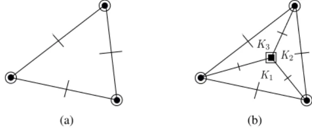
Figure 1. The HCT element (a) and the HCT element in detail (b).
2.3 Space discretization: HCT elements
The solution of (13) belongs to C0pr0, T s; V q X C1pr0, T s; Hq, thus we are led to select finite elements of class C1; in particular, we will use HCT elements.
Let Thdenote a regular mesh in the sense of Ciarlet [7, 19] of the domain Ω, K P Th the typical element of Th and Xha finite element space. Moreover, let PK “ tvh|K : vhP Xhu. We recall the following result of [7].
Theorem 2.5. Assume that the inclusions PK Ă H2pKq for all K P Th and XhĂ C1pΩq hold. Then the following inclusions hold:
XhĂ H2pΩq,
Xoh“ tvhP Xh: vh“ 0 on Γ0u Ă V2,
Xooh“ tvhP Xh: vh “ Bnvh“ 0 on Γ0u Ă V1.
Remark 2.6. The choices Vh“ Xoohfor pBCq1and Vh“ Xohfor pBCq2ensure hypotheses (19) to (21) of Theorem 2.3 to be satisfied [7].
Finite elements of class C1are rather complicated and time-consuming, and are not used too often in practical applications. We choose to start our experiments with such elements because the theory described is valid for conforming approx-imations. In this context, the HCT is one of the simplest C1elements (Fig. 1(a)). The set of degrees of freedom (twelve in total) is given by the values of a func-tion, as well as of its partial derivatives, at the three vertices and by the values of its normal derivatives at the midpoints of the sides. From an internal viewpoint, the HCT element is a composite element: a typical triangle K P This split into three sub-triangles Ki (i “ 1, 2, 3), the internal node usually corresponding to the barycenter of K (Fig. 1(b)). A polynomial of degree three is defined on each
sub-triangle, so that the space PK is given by
PK “ tp P C1pKq : p|KiP P3pKiq, 1 ď i ď 3u.
The condition p P C1pKq is realized by requiring the continuity of the three poly-nomial expansions and of their gradients at the barycenter (marked by a black square in Fig. 1(b)), and the continuity of their normal derivatives at the midpoints of the internal sides. Thus, the HCT element is a C1element as a whole, in the sense that a function and its first derivatives are continuous across the edges of any two adjacent elements of Th.
Let us now provisionally focus on the static counterpart of (13), namely, @v P V, apw, vq “ Lpvq, (23) where we have neglected time dependence. Notice that in this case the pivot space H is L2pΩq. The discrete version of (23) reads
I ÿ j“1
apϕi, ϕjqξj“ Lpϕiq, 1 ď i ď I.
The following theorem [7] yields an estimate of the error between whand w when HCT elements are employed in space discretization for (23).
Theorem 2.7. If the exact solution w P V of (23) is also in the space H4pΩq, then there exists a constantC ą 0 independent of h such that
}w ´ wh}H2pΩq ď Ch2|w|H4pΩq. (24)
Remark 2.8 (Implementation issues). In finite element methods, a quadrature scheme is needed to compute the coefficients apϕi, ϕjq and Lpϕiq, thereby re-sulting in an approximated bilinear form ahp¨, ¨q and in an approximated linear form Lhp¨q. Generally, integration over a mesh element is performed using a quadrature scheme for which all nodes are situated at the interior of the element. However, in the HCT case, a mesh element features internal interfaces between any two sub-triangles; at these interfaces, the continuity of second partial deriva-tives is not guaranteed. Hence, one should use a quadrature scheme that avoids nodes on any such interface. A solution is to integrate on each sub-triangle and then sum up the three contributions. Moreover, in order to apply the first Strang lemma [?, 7], we need that the bilinear form ahbe uniformly Vh-elliptic, i.e. Dα ą 0 : @vh P Vh, ahpvh, vhq ě α}vh}2. In our situation, if the space PK contains polynomials of degree at most k, a sufficient condition for ahto sat-isfy this property is that the quadrature scheme be exact for polynomials of degree 2k ´ 4 at least. This means that on each Ki Ă K, a quadrature formula exact at least for polynomials of degree two has to be used.
3
Numerical simulations
For what concerns the numerical treatment of problem (1)-(2), we will restrict our attention to an isotropic behavior; hence, the constitutive equation yielding M is
M “ ´D pp1 ´ νq∇∇u ` ν4u Iq , with D “ 2e 3E
3p1 ´ ν2q (25) the flexural rigidity of the plate, E and ν being respectively Young’s modulus and Poisson’s ratio of the material.
We perform numerical tests using the software package FreeFEM++ 3.42 (see [13]), in which HCT elements have been implemented along with an adequate quadrature formula for their use. We will consider two situations:
p1q Ω“ tpx, yq P R2: x2` y2ă R2u, Γ0“ BΩ and pBCq1,
i.e. a circular plate of radius R clamped all over the lateral surface; p2q Ω“ p0, aq ˆ p0, bq with a, b ą 0, Γ0“ BΩ and pBCq2,
i.e. a rectangular plate simply supported all over the lateral surface. In both situations we assume m “ 0, and in order to get coherent results we fix once and for all the following set of data:
R “ 5 cm, a “ 6 cm, b “ 8 cm, e “ 1 mm
ρ “ 5600 kg{m3, E “ 136 GP a, ν “ 0.3, pi.e. D “ 99.63 N ¨mq.
(26)
3.1 Statics
In each of the following test cases, we consider nested meshes in order to determine the behavior of the relative error in H2pΩq-norm with respect to the meshsize h; of course, mesh refinement is uniform.
3.1.1 Boundary conditions pBCq1 The problem formulation reads in this case
#
D44w “ f0 in Ω, w “ 0, Bnw “ 0 on BΩ,
(27)
with f0a constant; the closed-form solution of (27) is given in this case by wpx, yq “ f0
64DpR 2
Table 1. Variation of the H2-norm of the relative error with the number of finite
elements for w given by (28), along with the corresponding number of degrees of freedom.
Relative error in H2-norm 0.75% 0.2% 0.06% 0.01%
Number of finite elements 111 444 1776 7104 Number of degrees of freedom 386 1435 5531 21715
Table 1 shows that the variation of the H2-norm of the error with respect to the number of finite elements (and thus to the meshsize) is in agreement with error estimate (24), i.e. quadratic. A different simulation where the exact solution is non-polynomial, namely, wpx, yq “ f0
64DpR
2´ px2` y2qq2sinpaxq, gives similar results.
3.1.2 Boundary conditions pBCq2 The problem formulation is
$ & % D44w “ f0sin ´π ax ¯ sin ´π by ¯ in Ω, w “ 0, Mn ¨ n “ 0 on BΩ, (29)
The closed-form solution is given by
wpx, yq “ W0sin ´π ax ¯ sin ´π by ¯ , W0“ f0 π4D ˆ 1 a2` 1 b2 ˙´2 . (30)
The variation of the relative error is shown in Table 2, and once more the conver-gence is quadratic.
Table 2. Variation of the relative error in H2-norm with the number of finite elements
for w given by (30), along with the corresponding number of degrees of freedom.
Relative error in H2-norm 0.4% 0.1% 0.03% 0.009%
Number of finite elements 212 848 3392 13568 Number of degrees of freedom 719 2707 10499 41347
3.1.3 L-shaped clamped plate
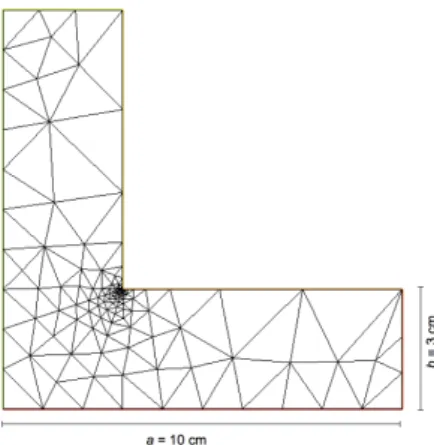
To further test the effectiveness of HCT elements, we also performed a numerical simulation in the case of an L-shaped clamped plate, i.e. with boundary conditions pBCq1. Table 3 shows the variation of the relative error in H2-norm. Since the
Figure 2. L-shaped domain.
closed-form solution is not known in this case, comparison has been made with a numerical solution obtained on a fine adapted mesh, consisting of 137232 elements (meshsize 0.08 mm). Computations have been carried out, again, with nested meshes, taking into account the singularity at the inside corner with a suitably-refined initial mesh. The corvergence rate turns out to be slightly slower than quadratic (1.74). Since the solution has very large variations around the inside corner, adaptive mesh refinement is necessary; however, such numerical aspects are beyond the scope of this paper.
Table 3. Variation of the H2-norm of the relative error with the number of finite
elements for w given by (28), along with the corresponding number of degrees of freedom.
Relative error in H2-norm 24.3% 7.3% 2.2% 0.8%
Number of finite elements 258 1032 4128 16512 Number of degrees of freedom 869 3283 12755 50275
3.2 Dynamics
In order to test the accuracy of the Newmark midpoint method combined with HCT elements, we consider the time evolution of the transverse displacement t ÞÑ whpx0, y0; tq, where px0, y0q is the center of the plate; we consider nested meshes in the two cases pBCq1and pBCq2. The data set is given in (26). We consider an exact solution of the form wpx, y; tq “ kpx, yq sinpβtq, where β is a constant1,
1 We obtained similar results for time dependencies of the form t2
and we take into account the evolution of the relative error εhptq “ $ ’ & ’ % ˇ ˇ ˇ ˇ whpx0, y0; tq ´ wpx0, y0; tq wpx0, y0; tq ˇ ˇ ˇ ˇ if t ą 0, wpx0, y0; tq ‰ 0, 0 if t “ 0. (31)
Since convergence occurs only for 0 ă t ď T where T is fixed, we precise in each example the value of T .
3.2.1 Influence of space discretization
In this section we fix once and for all the time-step to ∆t “ 0.01 s, and we point out the influence of space discretization.
Boundary conditions pppBCqqq1 The function wpx, y; tq “ f0 64DpR 2 ´ px2` y2qq2sinpβtq, (32) with f0a constant, is solution to the problem
$ ’ ’ ’ ’ ’ & ’ ’ ’ ’ ’ % 2eρ :w ´ 2e 3 3 ρ 4 :w ` D44w “ f in Ω ˆ p0, T q, w0px, yq “ 0, w1px, yq “ f0β 64DpR 2 ´ px2` y2qq2 in Ω, w “ 0, Bnw “ 0 on BΩ, with f px, y; tq “ ´β 2f 0eρ 96D ´ 3pR2´ px2` y2qq2` 8e2pR2´ 2px2` y2qq ¯ sinpβtq ` f0sinpβtq.
The evolution of the error given by (31) is shown in Fig. 3(a), and it reflects the expected behavior: the error evolution is attenuated upon refining the mesh.
Boundary conditions pppBCqqq2 The function wpx, y; tq “ W0sin ´π ax ¯ sin ´π by ¯ sinpβtq, (33)
with W0as in (30), is solution to the problem $ ’ ’ ’ ’ & ’ ’ ’ ’ % 2eρ :w ´ 2e 3 3 ρ 4 :w ` D44w “ f in Ω ˆ p0, T q, w0px, yq “ 0, w1px, yq “ βW0sin ´π ax ¯ sin ´π by ¯ in Ω, w “ 0, Mn ¨ n “ 0 on BΩ, with f px, y; tq “ “ ´2β 2a2b2f 0e`b2e2π2` a2p3b2` e2π2q ˘ 3π4Dpa2` b2q2 ρ sin ´π ax ¯ sin ´π by ¯ sinpβtq` ` f0sin ´π ax ¯ sin ´π by ¯ sinpβtq.
The evolution of the relative error given by (31) is shown in Fig. 3(b). Let us remark that the behavior of the error corresponding to the finest mesh (represented by a red line) is in this case almost imperceptible, inasmuch as it is very close to zero. Also, notice that the convergence is in this case remarkably faster than in Fig. 3(a); this can be related to the fact that no approximation error concerning the domain geometry is committed, unlike the case of pBCq1, where the domain under consideration is a circle.
3.2.2 Influence of time discretization
In this section we consider two different values of the time-step ∆t (namely, 0.01 s and 0.05 s) in order to point out the influence of this parameter.
In the case of pBCq2, when the source term vanishes (f ” 0), the closed-form solution to the dynamic problem can be obtained by separation of variables. Indeed, one has the Fourier development
wpx, y; tq “ ÿ m,nPN `g1 mncospωmntq ` gmn2 sinpωmntq ˘ sin ´mπ a x ¯ sin ´nπ b y ¯ , where ωmn “ π2 ˆ m2 a2 ` n2 b2 ˙g f f e D 2eρ `23π2e3ρ´m2 a2 ` n2 b2 ¯ ,
and coefficients g1mn and g2mnare determined by initial conditions. We consider then the following situation:
w0px, yq ” 0, and w1px, yq “ α sin ´π ax ¯ sin ´π by ¯ ,
0 0.02 0.04 0.06 0.08 0.1 0.12 0 0.5 1 1.5 2 2.5 3 3.5 0 0.02 0.04 0.06 0.08 0.1 0.12 0 0.5 1 1.5 2 2.5 3 3.5 0 0.02 0.04 0.06 0.08 0.1 0.12 0 0.5 1 1.5 2 2.5 3 3.5 Time (s) Relat ive error (a) 0 0.01 0.02 0.03 0.04 0.05 0 0.5 1 1.5 2 2.5 3 3.5 0 0.01 0.02 0.03 0.04 0.05 0 0.5 1 1.5 2 2.5 3 3.5 0 0.01 0.02 0.03 0.04 0.05 0 0.5 1 1.5 2 2.5 3 3.5 Time (s) Relat ive error (b)
Figure 3. Evolution of the relative error t ÞÑ εhptq with px0, y0q “ p0, 0q for
pBCq1(a) (continuous line: 27 elements; dashed line: 108 elements; red line: 432
elements), and with px0, y0q “ pa{2, b{2q for pBCq2(b) (continuous line: 12
ele-ments; dashed line: 48 eleele-ments; red line: 192 elements). In both cases, β “ 1 s´1
and T “ 3.5 s. In both cases, all three evolutions become slightly irregular (more remarkably in case (b), with the largest number of elements) when t is close to π; indeed, gpπq “ 0 for β “ 1 s´1.
in which case the exact solution is
wpx, y; tq “ α ω11 sin ´π ax ¯ sin ´π by ¯ sinpω11tq.
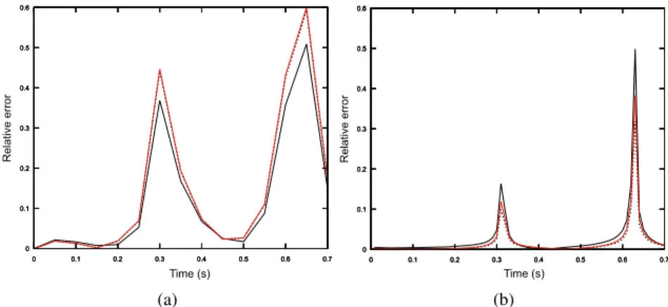
Given that the exact solution is p2π{ω11q-periodic in time, in order to test our nu-merical method we consider a reasonable value of ω11; say, ω11 “ 10 s´1. The evolution of the relative error, given by (31), is shown in Fig. 4(a) for a time-step ∆t “ 0.05 s and in Fig. 4(b) for a time-step ∆t “ 0.01 s. For ∆t “ 0.05 s, the obtained behavior is unexpected: mesh refinement results in an amplification of the relative error ; decreasing the time-step to ∆t “ 0.01 s yields the expected behavior. Indeed, note that the period τ corresponding to ω11 “ 10 s´1is approx-imately equal to 0.63 s, so that the ratio ∆t{τ is about 0.08 for ∆t “ 0.05 s and about 0.01 for ∆t “ 0.01 s. The influence of such ratio is well-known in the case of Newmark’s midpoint method (see, e.g., [12]).
0 0.1 0.2 0.3 0.4 0.5 0.6 0 0.1 0.2 0.3 0.4 0.5 0.6 0.7 0 0.1 0.2 0.3 0.4 0.5 0.6 0 0.1 0.2 0.3 0.4 0.5 0.6 0.7 0 0.1 0.2 0.3 0.4 0.5 0.6 0 0.1 0.2 0.3 0.4 0.5 0.6 0.7 Time (s) Relat ive error (a) 0 0.1 0.2 0.3 0.4 0.5 0.6 0 0.1 0.2 0.3 0.4 0.5 0.6 0.7 0 0.1 0.2 0.3 0.4 0.5 0.6 0 0.1 0.2 0.3 0.4 0.5 0.6 0.7 0 0.1 0.2 0.3 0.4 0.5 0.6 0 0.1 0.2 0.3 0.4 0.5 0.6 0.7 Time (s) Relat ive error (b)
Figure 4. Evolution of the relative error t ÞÑ εhptq , with px0, y0q “ pa{2, b{2q,
for a vanishing initial displacement and a nonzero initial velocity, for a time-step ∆t “ 0.05 s (a) and a time-step ∆t “ 0.01 s (b). Continuous line: 28 elements; dashed line: 112 elements; red line: 448 elements. In both cases, α “ 1 cm{s and T “ 0.7 s.
Concluding remarks
We have pointed out the importance of our choice of spaces V and H, required for the treatment of the rotational inertia term, not only in the proof of the problem’s well-posedness, but also in error estimates concerning our numerical method. Our simulations, performed using FreeFEM++ 3.42 show that the presence of the ro-tational inertia term does not affect the efficiency of the Newmark time discretiza-tion method combined with conforming finite elements such as HCT elements. We have tested the implementation of such elements in three cases: clamped cir-cular plate, simply supported rectangular plate and L-shaped clamped plate. In all these cases, our numerical experiments validate the convergence rate of the error predicted by the theory. As is well-known, HCT elements are computationally expensive; it would then be of interest to use nonconforming space discretization methods (mixed or hybrid) [4,17], such as HHO methods [8,9]. The application of such methods to plate problems seems particularly interesting and will be carried out in a forthcoming work.
Bibliography
[1] G. Allaire, Numerical Analysis and Optimization, Oxford University Press (2007). [2] G. A. Baker, Error estimates for finite element methods for second order hyperbolic
equations, SIAM J. Numer. Anal. 13 (1976), 564–576.
[3] J.-L. Batoz, K.-J. Bathe, L.-W. Ho, A study of three–node triangular plate bending elements, Internat. J. Numer. Methods Engrg. 12 (1980), 1771–1812.
[4] D. Boffi, F. Brezzi, M. Fortin, Mixed finite element methods and applications, Springer–Verlag (2013).
[5] F. Brezzi, M. Fortin, Mixed and hybrid finite element methods, Springer Science & Business Media (2012).
[6] F. Bonaldi, G. Geymonat, F. Krasucki, M. Serpilli, An asymptotic plate model for magneto-electro-thermo-elastic sensors and actuators, Math. Mech. Solids (2015), published online. DOI: 10.1177/1081286515612885.
[7] P. G. Ciarlet, The Finite Element Method for Elliptic Problems, SIAM (2002). [8] D. A. Di Pietro, A. Ern, S. Lemaire, An Arbitrary-Order and Compact-Stencil
Dis-cretization of Diffusion on General Meshes Based on Local Reconstruction Opera-tors, Comput. Methods Appl. Math. 14 (2014), 461–472.
[9] D. A. Di Pietro, A. Ern, A hybrid high-order locking-free method for linear elasticity on general meshes, Comput. Methods Appl. Mech. Engrg. 283 (2015), 1–21. [10] R. Dautray, J.-L. Lions, Mathematical Analysis and Numerical Methods for Science
and Technology, Volume 5 – Evolution Problems I, Springer-Verlag (2000).
[11] T. Dupont, L2–Estimates for Galerkin Methods for Second Order Hyperbolic Equa-tions, SIAM J. Numer. Anal. 10 (1973), 880–889.
[12] M. Géradin, D. J. Rixen, Mechanical Vibrations: Theory and Application to Struc-tural Dynamics, John Wiley & Sons (2015).
[13] F. Hecht, New development in FreeFem++, J. Numer. Math. 20 (2012), 251–265. [14] T. J. R. Hughes, The finite element method: linear static and dynamic finite element
analysis, Courier Corporation (2012).
[15] J.-L. Lions, E. Magenes, Non–Homogeneous Boundary Value Problems and Appli-cations, Springer-Verlag (1972).
[16] R. D. Mindlin, Influence of rotatory inertia and shear on flexural motions of isotropic, elastic plates, Journal of Applied Mechanics 18 (1951), 31–38.
[17] A. Quarteroni, A. Valli, Numerical Approximation of Partial Differential Equations, Springer-Verlag (2008).
[18] A. Raoult, Construction d’un modèle d’évolution de plaques avec terme d’inertie de rotation, Ann. Mat. Pura Appl. CXXXIX (1985), 361–400 (French).
[19] P. A. Raviart, J. M. Thomas, Introduction à l’analyse numérique des équations aux dérivées partielles, Masson (1983).
[20] J. W. S. Baron Rayleigh, The Theory of Sound, 2nd ed., 1894, reprinted Dover edition (1945).
[21] G. Strang, G. J. Fix, An Analysis of the Finite Element Method, Prentice-Hall (1973).
Author information
Francesco Bonaldi, Institut Montpelliérain Alexander Grothendieck, UMR-CNRS 5149, Université de Montpellier, Place Eugène Bataillon, 34095 Montpellier Cedex 5, France. E-mail: [email protected]
Giuseppe Geymonat, Laboratoire de Mécanique des Solides, UMR-CNRS 7649, École Polytechnique, CNRS, Université Paris-Saclay,
Route de Saclay, 91128 Palaiseau Cedex, France. E-mail: [email protected]
Françoise Krasucki, Institut Montpelliérain Alexander Grothendieck, UMR-CNRS 5149, Université de Montpellier, Place Eugène Bataillon, 34095 Montpellier Cedex 5, France. E-mail: [email protected]
Marina Vidrascu, REO project-team, Inria de Paris, 2 rue Simone Iff Voie DQ12, 75012 Paris, France. Laboratoire Jacques-Louis Lions, UPMC Univ. Paris 6, Sorbonne Universités, 4 Place Jussieu, 75252 Paris Cedex 5, France.