UNIVERSITÉ DU QUÉBEC À MONTRÉAL
EFFETS SIMPLES ET CUMULÉS DES PERTURBATIONS ET DES STRESS MULTIPLES SUR LES COMMUNAUTÉS BENTHIQUES INTERTIDALES :
RÔLE DES MACROPHYTES
THÈSE PRÉSENTÉE
COMME EXIGENCE PARTIELLE DU DOCTORAT EN BIOLOGIE
EXTENSIONNÉE À
L’UNIVERSITÉ DU QUÉBEC À CHICOUTIMI
PAR
STÉPHANIE CIMON
REMERCIEMENTS
Je tiens d’abord à remercier mon directeur de thèse, Mathieu Cusson, d’avoir eu la confiance de passer avec moi de l’initiation à la recherche jusqu’à la thèse de doctorat. Cette certitude qu’il a démontrée à mon égard a énormément joué au niveau de ma confiance pour accomplir un tel projet. Les bourses auxquelles j’ai eu accès m’ont permis d’entreprendre ce projet d’envergure. Du tout début, son soutien dans ces demandes a été primordial parce que ce n’est pas donné à tout le monde de bien les faire. Tout en me guidant, Mathieu m’a laissé m’approprier mon doctorat tout en me permettant de regretter certains de mes choix. Merci à Isabelle Côté de l’Université Simon Fraser, Alison Derry de l’UQAM et Christian Nozais de l’UQAR d’avoir accepté de faire partie de mon jury. Les conversations lors de la soutenance ont été plus qu’agréables.
Nos différentes collaborations ainsi que les bourses que Mathieu et moi avons obtenues m’ont permises d’effectuer deux stages dans des laboratoires externes. I want to thank Prof Peter Petraitis for his warm welcome in his lab at the University of Pennsylvania where he introduced me to R. I want to thank Prof Jay Stachowicz for welcoming me into his lab at the University of California, Davis, and at the Bodega Marine Laboratory. While in Davis, I developed the database of my last chapter and was able to exchange with Jay’s graduate students. Thank you, Melissa, Matt and Nicole for precious conversations and for bringing me to visit your field. While in California, I have had the positive experience to visit Prof Kevin Hovel and had the opportunity to discuss my results. Pour ces diverses expériences, je remercie Québec-Océan et le Fonds de recherche Nature et technologies du Québec (FRQNT) pour les bourses de stage.
Je veux remercier une collaboratrice qui est venue spécialement nous visiter à l’UQAC en avril 2019, Dr Francesca Rossi. Merci Francesca pour ta présence, nos discussions, ton enseignement, ta pédagogie et tes précieux conseils. Merci aussi d’avoir partagé ton expérience personnelle en regard à la science et à la recherche.
J’ai aussi eu le privilège de discuter ou de travailler avec certains professeurs de l’UQAC : Sergio Rossi, Annie Deslauriers et Romain Chesnaux. Merci Sergio pour tes ateliers sur l’écriture scientifique. Merci à Annie pour ta participation dans mon deuxième chapitre et merci à Romain d’avoir su répondre à des questions dont nous n’avions pas les réponses. Merci à Milla Rautio pour toutes les petites conversations personnelles et professionnelles et merci pour ta confiance et l’opportunité de te remplacer dans ton cours d’études biologiques sur le terrain. Merci beaucoup à Murray Hay de chez Maxafeau pour ses excellentes révisions linguistiques.
Mon doctorat s’est étiré sur plusieurs années. Effectivement, vu ma passerelle, ma maitrise fait partie de mon doctorat et on pourrait même dire que ce projet a duré trop longtemps! Ce projet a été mené sur trois étés de terrain intensif au rythme des marées soit ici un peu plus de 12 mois de travaux de terrain. Je veux remercier toutes les personnes qui de près ou d’un peu plus loin m’ont permises de réussir mes travaux de terrain. Je pense avant tout à Laetitia Joseph, Déborah Benkort et Carolane Valcourt. Léti, Deb et Caro, vous avez été mes fidèles compagnes lors des dures périodes de terrain. Vous avez partagé et mes hauts et mes bas, mais vous avez surtout toujours été là. Léti, tu m’as tellement aidé à débuter ma maitrise, sans toi ça n’aurait pas été pareil; merci pour ton organisation, ton originalité et ta passion pour le travail bien fait. Merci à ma petite Deb pour ton amitié sans frontières et avoir transformé un été de terrain sans fin en une expérience positive et inoubliable. Un merci particulier à Caro pour avoir survécu aux horaires de fous (un mois sans un seul congé où les plus petites journées de travail étaient de 10h!) qu’on a eu même si ce n’était pas lié à mon doctorat
lui-même; je me rappellerai toujours cette nuit où on s’est levées autour de 1-2h du matin pour aller relever la prédation de nos crabes, le tout terminé avec une coupe de vin pendant que le soleil se levait avant de retourner se coucher pour retourner travailler à la marée basse suivante! Merci Caro, ça n’a pas été facile ni pour toi ni pour moi, mais au moins on était ensemble. Merci Caro et David de m’avoir accueillie chez vous un été de temps d’ailleurs. Merci aussi aux autres personnes assez courageuses pour faire du terrain avec moi : Amy Lavoie, Julie Lemieux, David-Alexandre Gauthier, Guillaume Grosbois, Gabrielle Larocque, Maxime Wauthy, Sabrina Pelletier, Yves Valcourt, David Villeneuve, Julius Ellrich et Aurélie Guillou. Merci pour les beaux moments passés ensemble, je recommencerais ces aventures n’importe quand avec vous.
Qui dit échantillonnage dit tri et analyses. Je veux remercier tout spécialement Anne-Lise Fortin et Claire Fournier pour leur aide sans pareil. Anne-Anne-Lise, ton grand cœur et ton amour pour le travail bien fait et les laboratoires rangés m’ont énormément aidé et m’ont appris à organiser ma prise de données. Merci pour tous les petits services rendus même si ce n’était pas dans ta définition de tâches, cela a été plus qu’apprécié. Claire, merci de toujours être là pour nous dépanner ou prêter du matériel. Je dois encore une fois souligner le travail exemplaire de Caro ici. Merci Caro pour ta bonne humeur et ton dévouement. Merci à Deb qui a passé de nombreuse après-midi et plusieurs journées entières à trier des échantillons avec moi en laboratoire. Merci aussi à Tobinou, Gigi et Maxou pour leur disponibilité à me dépanner, et ce, à n’importe quel moment que ce soit pour transporter du matériel, mesurer la croissance des zostères ou encore faire des filtrations. Merci à Tobias de m’avoir enseigné comment utiliser le spectrophotomètre et son logiciel… deux fois plutôt qu’une! Merci à Gabrielle qui est venue m’aider un peu et apprendre qui étaient les petites bêtes que je triais. Merci à Jessica Tremblay et Guillaume Bonvalot-Maltais d’avoir enduré le bruit assourdissant de la mise en poudre de zostères. Merci à Marie-Pier Fournier de m’avoir non
seulement enseigné, mais accompagné dans mes extractions de glucides non structuraux. Merci à Laetitia et Julie pour votre aide quant à la diversité, la façon de la calculer et les bases de l’utilisation du logiciel PRIMER & PERMANOVA. Special thanks to Prof Marti Anderson who taught a workshop on the use of that same software but was also able to answer so many of my questions and got me so much more excited about multivariate statistics. Merci également à David Émond pour les réponses claires quant à mes questions statistiques. À tous, vous avez embelli de nombreuses heures et journées de laboratoire et d’analyses.
D’autres personnes ont aussi joué un rôle à l’université. Je pense à Dominique Simard qui est toujours présente pour répondre à nos questions d’ordre administratif. Je pense aussi à Germain Savard pour les beaux sourires et les blagues quand on se croise dans les couloirs. Je pense à toutes ces personnes que je croise de temps à autre et avec qui j’ai notamment des discussions de couloir, merci à vous tous!
Je tiens aussi à remercier mes collègues lointains Annie, Charlotte, David, Elliot, Kevin, Lupita, Manon, Marie et Valérie pour le soutien et les échanges enrichissants à chacune de nos rencontres. Grâce à vous, je me suis sentie moins seule dans mon monde d’écologie marine. Merci en particulier à Valérie pour ton partage de connaissances et codes pour les traits biologiques.
À tous mes collègues et amis, je dis merci : à Crysta et Pénélope pour vos beaux sourires; à Fanny, Valentine, Diamondra et Anne pour votre présence au bureau et votre humanité; à Mireille pour ta bonne humeur; à Sonya pour les discussions sur la vie et ta sincérité; à Pierre, car tu es de loin ma princesse favorite; à Laurence pour ta candeur, ton amour et nos discussions variées; à Minh Vu pour me loger, ta bonne volonté et ton calme; à Emilie pour une amitié de longue durée qui me rappelle d’où je viens; to
Christel and Sonia for joining the benthic team, your empathy and your support; à Paola pour le sport et ta bienveillance; à Laetitia et Guy parce que vous incarnez l’amour pur et pour Game of Thrones; à Xavier pour ton enthousiasme et les soirées de jeux; à Winna et Tony pour votre loyauté, votre affection et votre bonté sans fin; à Miguel pour ta sensibilité, ta compréhension et la folie totale; to Melissa and Nicole for your positive attitude and your focus; à Julie et Hélène pour vos fous rires hilarants à faire pleurer de joie; à Amy pour ton ouverture et ta sagesse; à Lupita, Carla, Leo, Caro S., Victor, Kathy, gros Ben, Hassen, Kevin et Benoit pour le délire de la maison blanche; à Caro V. pour ton authenticité, ta jovialité et ta raison; à Deb pour ta sensibilité, ta dévotion, ton énergie et ton sens de l’humour; à Henrique pour les conversations, la chorale et ton grand cœur; à Max W. pour ton éternel soutien et ta complicité que ce soit au labo, au bureau, à la maison ou dans les loisirs; à Guillaume pour les cafés, les randos, les oiseaux et les marmottes, ton écoute et ta passion; à Tobias pour la folie, ta disponibilité, ton amitié inconditionnelle, tes mots inventés, les cafés et les déjeuners sur mon balcon; à Gabrielle pour ta détermination, ton dynamisme, ta sensibilité et ta personnalité; à Stéphane pour ta compassion, le yoga, ton esprit et ton soutien; and to Elizabeth, Deb, Margaret, Alice and Kate for welcoming me into your home and hearts as well as treating me as one of your own for four months. Merci à toute la chorale des étudiants de l’UQAC pour le partage d’une passion et mettre du soleil dans mes longues semaines. Finalement, merci aux « tomateuses », Marie-Michelle, Parinaz et Roxanne, pour avoir rendu les derniers milles de cette thèse plus agréables dans le contexte d’isolement social dû à la pandémie.
Depuis toujours, ma famille a été là pour me soutenir et m’encourager. Bien que je me rende mal compte de l’accomplissement qu’est cette thèse, la fierté que me portent mes parents et mes sœurs illustre très bien ma persévérance scolaire et ma réussite en tant qu’étudiante-chercheure. Merci à ma famille et Maxime de m’avoir accompagné et soutenu tout au long de ma thèse et des péripéties de maladies.
Je veux également remercier les organismes subventionnaires qui m’ont personnellement financée sans qui le projet et ses à-côtés n’auraient pas été possibles soit le FRQNT et le CRSNG, ainsi que Québec-Océan, le MAGE-UQAC et les services aux étudiants. Je remercie finalement Christopher McKenzie et l’Institut Maurice-Lamontagne pour l’accès à leurs laboratoires à Mont-Joli.
TABLE DES MATIÈRES
REMERCIEMENTS ... II TABLE DES MATIÈRES ... VIII LISTE DES FIGURES ... XII LISTE DES TABLEAUX ... XVII RÉSUMÉ ... XXIV ABSTRACT ... XXVII
INTRODUCTION GÉNÉRALE ... 1
0.1 Mise en contexte ... 1
0.2 État des connaissances ... 7
0.2.1 La biodiversité ... 7
0.2.2 Stabilité des communautés ... 7
0.2.3 Les espèces structurantes ... 13
0.2.4 Contrôles descendant et ascendant ... 17
0.3 Importance de mon doctorat ... 21
0.4 Objectifs et hypothèses ... 24
0.4.1 Chapitre I ... 24
0.4.2 Chapitre II ... 25
0.4.3 Chapitre III ... 27
0.5 Structure de la thèse ... 28
0.5.1 Chapitre I : Impact of multiple disturbances and stress on the temporal trajectories and resilience of benthic intertidal communities. ... 28
0.5.2 Chapitre II : Multiple stressors and disturbance effects on eelgrass and epifaunal macroinvertebrate assemblage structure. ... 28
0.5.3 Chapitre III : Site dependent effects of proximity to patch edge and eelgrass complexity on epifaunal communities within Zostera marina L.
meadows ... 29
CHAPITRE I IMPACT OF MULTIPLE DISTURBANCES AND STRESS ON THE TEMPORAL TRAJECTORIES AND RESILIENCE OF BENTHIC INTERTIDAL COMMUNITIES ... 30 1.1 Abstract ... 31 1.2 Introduction... 32 1.3 Methods ... 36 1.3.1 Study site ... 36 1.3.2 Experimental design ... 37 1.3.3 Sampling ... 40 1.3.4 Data analysis ... 41 1.4 Results ... 44
1.4.1 Effects of single and multiple stresses ... 44
1.4.2 Community trajectory over time and community resilience ... 48
1.5 Discussion ... 54
1.5.1 Structure, abundance, and diversity of communities ... 55
1.5.2 Community resilience ... 58
1.6 Concluding remarks ... 59
1.7 Acknowledgments ... 60
CHAPITRE II MULTIPLE STRESSORS AND DISTURBANCE EFFECTS ON EELGRASS AND EPIFAUNAL MACROINVERTEBRATE ASSEMBLAGE STRUCTURE ... 61 2.1 Abstract ... 62 2.2 Introduction... 62 2.3 Methods ... 66 2.3.1 Study site ... 66 2.3.2 Experimental design ... 67
2.4 Sampling and sorting ... 69
2.4.1 Eelgrass measurements ... 69
2.4.2 Epibenthic community measurements ... 70
2.6 Results ... 73
2.6.1 Stressors effects on eelgrass ... 74
2.6.2 Stressor effect on associated epibenthic communities ... 77
2.7 Discussion ... 82
2.7.1 Stressor effects on eelgrass ... 83
2.7.2 Stressor effect on associated epibenthic communities ... 86
2.8 Concluding remarks ... 89
2.9 Acknowledgments ... 90
CHAPITRE III SITE DEPENDENT EFFECTS OF PROXIMITY TO PATCH EDGE AND EELGRASS COMPLEXITY ON EPIFAUNAL COMMUNITIES WITHIN ZOSTERA MARINA L. MEADOWS ... 91
3.1 Abstract ... 92
3.2 Introduction... 93
3.3 Methods ... 97
3.3.1 Biological trait approach ... 100
3.3.2 Statistical analysis ... 102
3.4 Results ... 103
3.4.1 Initial eelgrass measures and epiphytic algae ... 103
3.4.2 Total epifaunal densities and species richness ... 104
3.4.3 Functional diversity ... 107
3.4.4 Biological traits occurrence structure... 110
3.5 Discussion ... 116
3.5.1 Effects on diversity-related indices ... 117
3.5.2 Effects on functional diversity and biological traits ... 119
3.6 Concluding remarks ... 121
3.7 Acknowledgments ... 122
CONCLUSION GÉNÉRALE ... 123
4.1 Retour sur les objectifs et hypothèses ... 123
4.2 Contributions majeures ... 127
4.2.1 La résistance et la résilience ... 127
4.2.2 Les macrophytes structurants ... 128
4.2.3 Les indices liés à la diversité ... 130
4.3 Limites de l’étude et perspectives... 131
4.4 Recommandations... 135
ANNEXES ... 138
Annexe A – Informations supplémentaires concernant le Chapitre I : Cimon, S. and Cusson, M. 2018. Impact of multiple disturbances and stress on the temporal trajectories and resilience of benthic intertidal communities. Ecosphere 9. doi.org/10.1002/ecs2.2467 ... 139
Annexe B – Informations supplémentaires concernant le Chapitre II : Cimon, S., Deslauriers, A. and Cusson, M. Multiple stressors and disturbance effects on eelgrass and epifaunal macroinvertebrate assemblage structure... 143
5.2.2 Taxa found during sampling ... 143
5.2.3 Additional tables ... 144
5.2.4 Supplementary results: effects of treatments on species ... 146
5.2.5 SIMPER tables ... 147
5.2.6 Supplementary figures ... 150
Annexe C – Informations supplémentaires concernant le Chapitre III : Cimon, S., Hovel, K., Boyer, K.E., Duffy, J.E., Hereu, C.M., Jorgensen, P., Kiriakopolos, S., Pierrejean, M., Reynolds, P.L., Rossi, F., Stachowicz, J.J., Ziegler, S.L., Cusson, M. Site-dependent effects of proximity to patch edge and eelgrass complexity on epifaunal communities within Zostera marina L. meadows. ... 154
5.3.2 Biological traits occurrence detailed results ... 154
5.3.3 Supplementary tables and figures ... 158
LISTE DES FIGURES
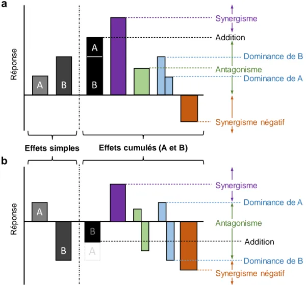
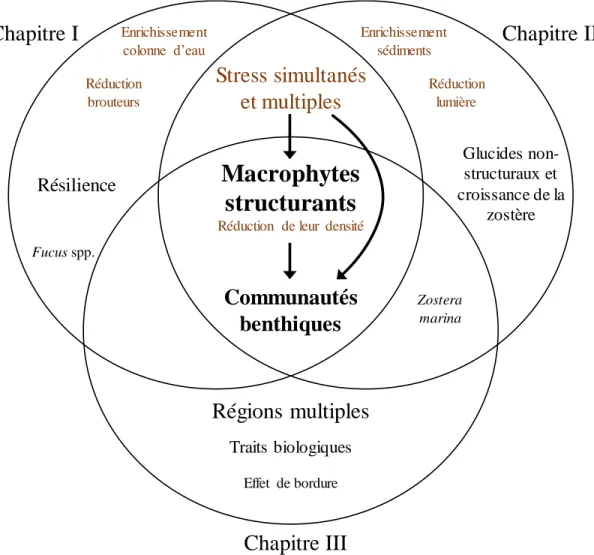
Figure 0.1. Représentations graphiques montrant les types d’effets cumulatifs possibles entre deux stress (A et B) : addition (noir), synergisme (violet), antagonisme (vert), dominance (bleu) et synergisme négatif (orange). (a) et (b) sont deux scénarios possibles utilisés à titre d’exemple. De façon générale, une interaction synergique aura lieu lorsque l’effet cumulé sera plus grand que l’effet anticipé de l’addition des réponses (a); un synergisme négatif, lorsque l’effet cumulé est de signe opposé à la réponse des stress (a); un antagonisme positif, lorsque l’effet cumulé est plus petit que l’effet anticipé additif (a,b); et dominant, lorsque l’effet n’est pas différent de l’un des deux stress (a,b). Les interactions sont un peu différentes lorsque les effets sont de sens opposé tel qu’en (b) : synergisme si la réponse est plus élevée que le stress A, relation antagoniste négative si la réponse cumulée est moins négative que l’addition des deux stresseurs, et synergisme négatif si la réponse est plus négative que celle du stress B. Figure modifiée de Côté et al. (2016). Consulter Galic et al. (2018) pour d’autres représentations graphiques semblables. ... 6 Figure 0.2. Diagramme conceptuel des trois chapitres de la thèse doctorale. L’élément central de la thèse est le rôle des macrophytes structurants (Fucus spp. ou Zostera
marina) sur les différentes mesures de biodiversité relatives aux communautés
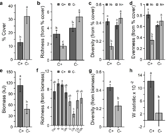
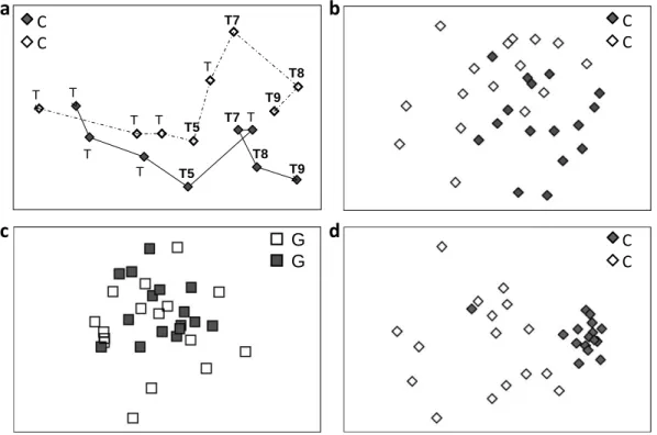
benthiques des habitats côtiers marins. À cela s’ajoute les effets des stress multiples sur les macrophytes structurants et leurs communautés associées aux chapitres I et II. De plus, la résilience des communautés est évaluée au chapitre I et des mesures sur les macrophytes structurants sont ajoutées au chapitre II. Quant au chapitre III, il évalue si les effets des macrophytes structurants sur les communautés associées varient en fonction des régions en utilisant une approche par traits biologiques. ... 23 Figure 1.1. Schematic of the experimental design showing the three stress treatments (canopy, grazer, nutrient enrichment; two levels each) following pretreatment (plots scraped to bare rock and then burned), and reference plots left untouched (see the Methods section for details). Bottom row shows letter codes for treatments with one, two, or three letters representing the quantity of stress applied. Ctrl and Ref represent Control and Reference, respectively. ... 39 Figure 1.2. Mean (±SE) values of (a) abundance in % cover, (b, f) species richness, (c, g) Simpson’s diversity index (1-), (d) Pielou’s evenness, (e) biomass (kJ), and (h) the W statistic among various treatments for non-manipulated species. Values are from data in percent cover from Period 8 (a–b), percent cover from Period 5 (c–d), biomass from Period 9 (e–g), and counts and biomass from Period 9 (h). Dark and light gray
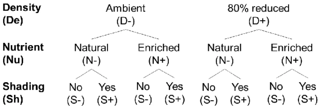
bars are the respective treatments with C+: canopy untouched; C-: canopy removed; G+: grazers untouched; G-: grazers reduced; N+: nutrients added; N- no nutrients added. See Fig. 1.1 for details of the different treatments in (f). The number of replicates used to obtain the averages were n = 16 in (a), (e), (g), and (h); n = 8 in (b), (c), and (d); n = 4 in (f). Different letters above the bars indicate significant differences (p < 0.05). ... 48 Figure 1.3. Non-metric multidimensional scaling (nMDS) plots illustrating the effect on community structure of (a) the canopy treatment across all periods (showing centroids), (b, d) the canopy treatment at Period 9, and (c) the grazer treatment at Period 8. Values were calculated based on Bray–Curtis similarities of the non-manipulated species based on percent cover data (a), (b), and (c) or biomass (d). C+: canopy untouched; C-: canopy removed; G-: grazers untouched; G+: grazers reduced. In (a), an asterisk (*) indicates a significant difference (p < 0.05) in community structure between C+ and C- at the given period. Stress from a to d: 0.07, 0.17, 0.19, and 0.12, respectively. ... 51 Figure 1.4. Community evolution over time. (a) Mean total abundance in percent cover of all species from visual observations in the field by treatment (n = 4). (b) Average dissimilarities between pairs of reference and treatment plots (n = 16) of each period for abundance in % cover structure of non-manipulated species. Light gray areas are 95% confidence intervals of the mean of reference plots (n = 4 in (a); within dissimilarities n = 6 in (b)). (b) Significant values between references and treatments are shown by filled circles (t-tests, p < 0.05). See Fig. 1.1 for treatments and definitions of C, G, N; number of letters in the treatment labels represents the amount of stress applied. ... 53 Figure 1.5. Second-stage nMDS ordination illustrating the change in average community structure patterns over time for each treatment (a) and Spearman correlations with controls (b) using non-manipulated species. (a) Second-stage nMDS is calculated from Spearman correlations of Bray–Curtis similarity coefficient matrices of average community structure pattern over time. Open circles represent single stressor treatments, gray circles represent two-stressor treatments, and black circles represent triple-stressor treatments. Stress = 0.08. (a,b) Ctrl and Ref refer to Control and Reference, respectively. See Fig. 1.1 for treatments and definitions of C, G, N; the number of these letters in the treatment labels represents the quantity of stress applied. ... 54 Figure 2.1. Schematic of the experimental design displaying the three stressor treatments (eelgrass shoot density reduction, sediment nutrient enrichment, shading, each with two levels; – stressor absent, + stressor present). ... 67 Figure 2.2. Mean (±SE) values of (a, e) eelgrass relative leaf elongation rate (day-1; RLE), (b) eelgrass shoot density, soluble sugars in (c) shoots and (g) root-rhizomes, starch in (d) shoots and (h) root-rhizomes, and (f) epiphyte load on shoots (chlorophyll
a; µg·g-1dw). Values are from Period 2. Gray and white bars are the respective
treatments with – stressor absent, + stressor present; D: eelgrass shoot density reduction, N: sediment nutrient enrichment, S: shading. The number of replicates used to obtain the averages was n = 20 in a, d, e, f, and g; n = 10 in c and h; and n = 5 in b. Different letters above bars indicate significant differences (p < 0.05, Tukey HSD). 77 Figure 2.3. Mean (±SE) values of epifaunal (a, e) abundances standardized per shoot dry weight (N·g-1dw), (b) species richness, (c, f) Pielou’s evenness, (d, g, h) Simpson’s
diversity. Values are from Period 2 except (c) which is from Period 1. Gray and white bars are the respective treatments with: – stressor absent, + stressor present; D: eelgrass shoot density reduction, N: sediment nutrient enrichment, S: shading. The numbers of replicates used to obtain the averages were n = 20 in (a), (c), (d), (e), (g) and (h); n = 10 in (b) and (f). Different letters above the bars indicate significant differences (p < 0.05). ... 82 Figure 3.1. Mean (±SE) values of (a, c, d) total epifaunal density (N∙g-1 macrophyte) and
(b) species richness. Values show the effect of position (a–b), density reduction (c), and the interaction between position and density reduction for MX region only (d). Bars are the respective treatment with E: Edge; I: Interior; 0: ambient eelgrass shoot density; 0.5: 50% density reduction; 0.8: 80% density reduction. The number of replicates used to obtain the averages was n = 21 in (a and c), n = 14 in (b), and n = 7 in (d). ... 107 Figure 3.2. Mean (±SE) values of (a) functional evenness and (b) Rao’s quadratic entropy. Values show the effect of complexity (a–b). Bars are the respective treatment with 0: ambient eelgrass shoot density; 0.5: 50% density reduction; 0.8: 80% density reduction. The number of replicates used to obtain the averages was n = 14 (a–b). Different letters indicate significant differences (p < 0.05). ... 109 Figure 3.3. Mean (±SE) values of (a) functional evenness and (b) Rao’s quadratic entropy. Values are showing effect of complexity (a-b). Bars are the respective treatment with 0: ambient eelgrass shoot density; 0.5: 50% density reduction; 0.8: 80% density reduction. The number of replicates used to obtain the averages was n = 14 (a-b). Different letters indicate significant differences (p < 0.05). ... 110 Figure 3.4. Proportions of each category of trait by position in each region showing (a) size, (b) life habits and movement, (c) feeding habits, (d) reproduction dispersal, and (e) larval feeding mode. Please refer to Table 3.1 for decoding trait categories acronyms. Bars are the respective treatment with E: Edge; I: Interior. ... 113 Figure 3.5. Proportions of each category of trait by complexity in each region showing (a) size, (b) life habits and movement, (c) feeding habits, (d) reproduction dispersal, and (e) larval feeding mode. Please refer to Table 3.1 for decoding trait categories acronyms. Bars are the respective treatment with 0: ambient eelgrass shoot density; 0.5: 50% density reduction; 0.8: 80% density reduction. ... 114
Figure 3.6. Principal coordinate ordinations illustrating the position effect on weighted trait occurrence structure (WTO) of (a) VA, (b) FR, (c) SF, and (d) MX. Values were calculated based on Euclidean distances of the WTO. Vectors are the more responsible traits for differences in position. Please refer to Table 3.1 for decoding trait categories. Only significant vectors were kept (p < 0.05). ... 115 Figure 3.7. Principal coordinate ordinations plots illustrating the effect on weighted trait occurrence structure (WTO) of the interaction of position and complexity in (a) FR and the effect of complexity in (b) MX, (c) QU and (d) VA. Values were calculated based on Euclidean distances of the WTO. Please refer to Table 3.1 for decoding trait categories acronyms. Vectors are the more responsible traits for differences in complexity. Only significant vectors were kept (p < 0.05). ... 116 Figure 5.1. Non-metric multidimensional scaling (nMDS) ordinations illustrating average community structure patterns over time for the different treatments (plain line) in comparison with the controls (dashed line) (a–h). Numbers along the lines represent periods. See Fig. 1.1 for treatments and the definitions of C, G, N; the number of letters (1–3; C,G,N) in the treatment labels represents the quantity of stress applied except for Ref, which represents the reference plots. Rho and p values have been calculated with Mantel-type tests using Spearman rank. In (h), circles represent a cluster group having an average 60% similarity. Stress from a to h: 0.09, 0.08, 0.13, 0.11, 0.08, 0.11, 0.10, and 0.08, respectively. ... 142 Figure 5.2. Mean (±SE) values of soluble sugars (mg·g-1dw) in (a) shoots and (c)
root-rhizomes, starch content (mg·g-1
dw) in (b) shoots and (d) root-rhizomes, and (e) relative
leaf elongation. The reported values are from Period 2. Gray and white bars are the respective treatments with D-: eelgrass shoot density untouched; D+: eelgrass shoot density reduced; S-: natural light; S+: shading. The numbers of replicates used to obtain the averages was n = 10. Different letters above the bars indicate significant differences (p < 0.05, Tukey HSD). ... 150 Figure 5.3. Principal component analysis (PCA) plot of normalized non-structural carbohydrates in shoots and root-rhizomes. Values are from Period 2. D-: eelgrass shoot density untouched; D+: eelgrass shoot density reduced; S-: natural light; S+: shading. Each bubble represents a plot. Bubble size is proportional to the relative leaf elongation rate (day-1; RLE)... 151
Figure 5.4. Mean (±SE) values of total raw abundance (a, d), biomass of Zostera
marina from epifaunal samples (b, e, g–i), (c, f) total abundance standardized per shoot
dry weight. Values are from Period 1, 2, and 3 in a–c, Period 1 in d–f, and Period 2 in g–i. D-: eelgrass shoot density untouched; D+: eelgrass shoot density reduced; N-: no nutrients added; N+: nutrients added; S-: natural light; S+: shading. The numbers of replicates used to obtain the averages were n = 20 in (a–c) and (g); n = 10 in (d–f) and (h); n = 5 in (i). Different letters above the bars indicate significant differences (p < 0.05; Tukey HSD for multiple comparisons). ... 152
Figure 5.5. Non-metric multidimensional scaling plots illustrating the effect (cf. Table 4 for details) on assemblage structure of (a, c, e) eelgrass shoot density reduction, (b) sediment nutrient enrichment, and (d) shading in Period 1 (a), Period 2 (b–d), and Period 3 (e). Values were calculated based on Bray-Curtis similarities of the dispersion-weighted and square root–transformed standardized abundance of species. Black and white symbols are the respective treatments with - stress absent, + stress present; D: eelgrass shoot density reduction, N: sediment nutrient enrichment, S: shading. ... 153 Figure 5.6. Mean (±SE) values of (a) eelgrass shoot density (N m-2), (b) eelgrass shoot biomass (g m-2), and (c) epiphyte load biomass (mg g-1shoot dw). Values are showing
effect of position. Bars are the respective treatment with E: Edge; I: Interior. The number of replicates used to obtain the averages was n = 21 in (a and c), n = 28 in (b) but n = 5 in interior and n = 13 in edge in FR, n = 26 in edge in SF and n = 23 in interior in VA. ... 184 Figure 5.7. Principal coordinate ordinations illustrating the distances among species using their biological traits by region. Values were calculated based on fuzzy calculated Gower’s distances using ‘dist.ktab’ in the ‘ade4’ R package. All trait categories are illustrated with vectors. Refer to Table 2 of the main text for decoding the trait categories and refer to Table S2 for decoding the species. ... 185 Figure 5.8. Metric multidimensional scaling (mMDS) of the estimated 95% region of bootstrap averages (n = 50) from replicates (Euclidean distances; square-root transformed WTO) of treatments (position × complexity) in France (FR; see Table 3.3h). Bootstrapping performed in m = 4 dimensional mMDS space. ... 186 Figure 5.9. Proportions of each category of trait by treatment (position and complexity) for France (FR) region showing (a) size, (b) life habit, (c) feeding habit, (d) reproduction mode, and (e) larval feeding mode. Please refer to Table 1 for decoding-trait categories. Bars are the respective treatment with E: Edge; I: Interior; 0: ambient eelgrass shoot density; 0.5: 50% complexity-reduced; 0.8: 80% complexity-reduced. ... 187
LISTE DES TABLEAUX
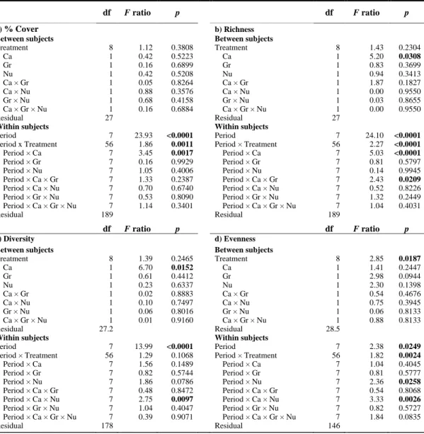
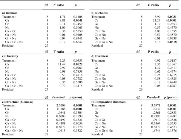
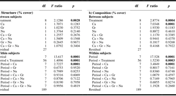
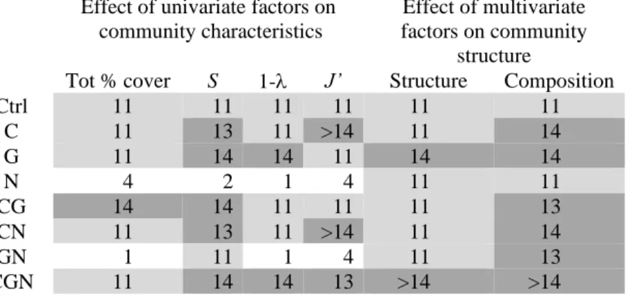
Table 1.1. Summary of RM ANOVAs showing the effects of treatment, full factorial contrasts of canopy (Ca), grazer (Gr), and nutrient enrichment (Nu) factors on abundance in % cover, richness, Simpson’s index of diversity, and Pielou’s evenness of non-manipulated species of the community for all periods. Significant values are shown in bold. ... 47 Table 1.2. Summary of (a–d) ANOVAs and (e–f) PERMANOVAs from biomass data obtained by destructive sampling (Period 9 only) showing the effects of treatment, full factorial contrasts of canopy (Ca), grazer (Gr), and nutrient enrichment (Nu) factors on biomass, richness, Simpson’s index of diversity, Pielou’s evenness, structure, and composition of the non-manipulated species of the community. Significant values are shown in bold. ... 49 Table 1.3. Summary of RM PERMANOVAs showing the effects of treatment and full factorial contrasts of canopy (Ca), grazer (Gr), and nutrient enrichment (Nu) factors on abundance structure and species composition for non-manipulated species of the community for all periods. Significant values are shown in bold. ... 50 Table 1.4. Recovery time (in months) of the non-manipulated species community in terms of diversity profile characteristics (total % cover; species richness S; evenness
J’; Simpson diversity 1-) and the structure (square root abundance) or composition
(presence/absence) for each treatment. Recovery was achieved when no significant differences (p > 0.05) were observed between a given treatment and the reference plots before the end of the experiment. If not reached by the end of the study, then the recovery time is deemed to be >14 months. Grayscale is based on controls (Ctrl) where no shading (white) represents cases where recovery happened faster than in the controls (light gray), and dark gray signifies where recovery was slower than observed in the control plots. Note the sampling gap between months 4 and 11 due to winter (i.e., it was not possible to determine recovery time values from months 5 to 10). See Fig. 1.1 for details regarding the treatment codes. ... 52 Table 2.1. Summary of the analyses of variance (ANOVAs) showing the effects of eelgrass shoot density reduction (De), sediment nutrient enrichment (Nu), and shading (Sh) factors on (a) relative leaf elongation rate (day-1;RLE), (b) eelgrass shoot density
(shoot·m-2; only effects of Nu and Sh), and (c) epiphyte load as chlorophyll a concentration (µgchl a·g-1dw) during Period 2 (see ‘Methods’). Significant values are
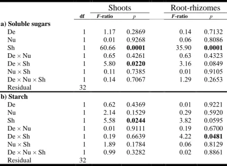
Table 2.2. Summary of the analyses of variance (ANOVAs) showing the effects of eelgrass shoot density reduction (De), sediment nutrient enrichment (Nu), and shading (Sh) factors on the soluble sugar and starch contents of shoots and root-rhizomes in Period 2 (see ‘Methods’). Significant values are shown in bold. ... 76 Table 2.3. Summary of the analyses of variance (ANOVAs) showing the effects of eelgrass shoot density reduction (De), sediment nutrient enrichment (Nu), and shading (Sh) factors on standardized abundance (N·g-1dw), richness, Pielou’s evenness, and
Simpson’s diversity index of associated epifauna for all sampling periods. Significant values are shown in bold. ... 80 Table 2.4. Summary of permutational analysis of variance (PERMANOVAs) showing the effects of eelgrass shoot density reduction (De), sediment nutrient enrichment (Nu), and shading (Sh) factors on the structure in standardized abundance (N·g-1
dw) and
composition (transformed into presence-absence) of associated epifauna for all sampling periods. Significant values are shown in bold... 81 Table 2.5. Summary of the type of interaction effect among eelgrass shoot density reduction (De), sediment nutrient enrichment (Nu), and shading (Sh) treatments. .... 81 Table 3.1. The five regions sampled in the study. Temperature and salinity were measured at low tide. MLLW: mean lower low water. The total richness is the total number of species used in the analysis for the all the samples in that region. No data available at this time where n.d. ... 99 Table 3.2. Biological traits and categories used to compare the species present in the five regions on a common basis to better measure species-habitat relationships. .... 101 Table 3.3. Summary of PER-ANOVAs showing the effects of position (Pos) and complexity (Com) on total density, richness, functional richness (FRic), functional evenness (FEve), functional divergence (FDiv), Rao’s quadratic entropy (RaoQ), functional redundancy, and biological weighted trait occurrence structure (PERMANOVA) of standardized species by region. Significant results are shown in
bold, while results in italics indicate that only ambient plots significantly differed from
the results here (cf. Annexe C: Table 5.29). ... 105 Tableau 4.1. Résumé des types d’interaction entre les divers stress pour les chapitres I et II : enlèvement de la canopée (Ca), réduction des brouteurs (Gr), enrichissement en nutriments (Nu), réduction en densité (De) et ombrage (Sh). Se référer aux différents chapitres pour les détails. Gris = absence d’effet. Noter que le chapitre III n’a pas présenté d’interaction entre les stress étudiés et qu’il est donc absent de ce tableau. ... 126 Table 5.1. List and classification of taxa found during all sampling periods at Sainte-Flavie, Quebec, Canada. Taxa marked with an asterisk were removed from the canopy-removed plots; taxa marked with a double asterisk were canopy-removed from the
grazer-reduced plots. Taxa marked with † and ‡ were respectively exclusively or mostly present in Period 9 when destructive sampling occurred (biomass). ... 139 Table 5.2. Summary of PERMANOVAs showing the effects of treatment and contrast of canopy (Ca) factor on the structure (in abundance % cover) for the non-manipulated species of the communities for all periods. Significant values are shown in bold. .. 140 Table 5.3. Summary of PERMDISP analysis (999 permutations were run) showing the effects of treatment and the three main factors on dispersion of the community structure of non-manipulated species from percent cover for all periods and from biomass at final sampling (Period 9). Significant values are shown in bold. ... 141 Table 5.4 List and classification of taxa found during all sampling periods at Pointe-aux-Outardes, Quebec, Canada. ... 143 Table 5.5. Summary of ANOVA showing the effects of sediment nutrient enrichment (Nu) and shading (Sh) factors on eelgrass shoot density for Period 0 and Period 3. Significant values are shown in bold. ... 144 Table 5.6. Summary of ANOVA showing the effects of eelgrass shoot density reduction (De), sediment nutrient enrichment (Nu), and shading (Sh) factors on epiphyte load at Period 1 (dry weight of epiphytes (g) / dry weight of Z. marina (g)). Significant values are shown in bold. ... 144 Table 5.7. Summary of PERMANOVAs showing the effects of eelgrass shoot density reduction (De), sediment nutrient enrichment (Nu), and shading (Sh) factors on normalized soluble sugars and starch for leaves and root-rhizomes separately using Euclidean distances at Period 2. Significant values are shown in bold. ... 145 Table 5.8. Summary of ANOVAs showing the effects of eelgrass shoot density reduction (De), sediment nutrient enrichment (Nu), and shading (Sh) factors on raw abundance of epifauna (N) and biomass of Z. marina (gdw) collected with epifaunal
samples at sampling periods 1 to 3. Raw abundances were log transformed while Z.
marina biomass were square-root transformed. Significant values are shown in bold.
... 145 Table 5.9. Summary of SIMPER (percentage of similarity) for eelgrass shoot density reduction in Period 1. Table shows species that cumulatively contribute up to 70% to the dissimilarity between treatments. D-: eelgrass shoot density untouched; D+: eelgrass shoot density reduced; Av. nb.: average number (abundance); Av. diss.: average dissimilarity; Diss/SD: dissimilarity divided by standard deviation; Contrib.%: percentage of contribution; Cum.%: cumulated percentage of contribution. Species in
bold have significant differences (p-values provided) of abundance between treatments
(t-test). ... 147 Table 5.10. Summary of SIMPER (percentage of similarity) for eelgrass shoot density reduction in Period 2. Table shows species that cumulatively contribute up to 70% to
the dissimilarity between treatments. D-: eelgrass shoot density untouched; D+: eelgrass shoot density reduced; Av. nb.: average number (abundance); Av. diss.: average dissimilarity; Diss/SD: dissimilarity divided by standard deviation; Contrib.%: percentage of contribution; Cum.%: cumulated percentage of contribution. Species in
bold have significant differences (p-values provided) of abundance between treatments
(t-test). ... 148 Table 5.11. Summary of SIMPER (percentage of similarity) for eelgrass shoot density reduction in Period 3. Table shows species that cumulatively contribute up to 70% to the dissimilarity between treatments. D-: eelgrass shoot density untouched; D+: eelgrass shoot density reduced; Av. nb.: average number (abundance); Av. diss.: average dissimilarity; Diss/SD: dissimilarity divided by standard deviation; Contrib.%: percentage of contribution; Cum.%: cumulated percentage of contribution. Species in
bold have significant differences (p-values provided) of abundance between treatments
(t-test). ... 148 Table 5.12. Summary of SIMPER (percentage of similarity) sediment nutrient enrichment in Period 2. Table shows species that cumulatively contribute up to 70% to the dissimilarity between treatments. N-: no nutrients added; N+: nutrients added; Av. nb.: average number (abundance); Av. diss.: average dissimilarity; Diss/SD: dissimilarity divided by standard deviation; Contrib.%: percentage of contribution; Cum.%: cumulated percentage of contribution. Species in bold have significant differences (p-values provided) of abundance between treatments (t-test). ... 149 Table 5.13. Summary of SIMPER (percentage of similarity) for shading in Period 2. Table shows species that cumulatively contribute up to 70% to the dissimilarity between treatments. S-: natural light; S+: shading; Av. nb.: average number (abundance); Av. diss.: average dissimilarity; Diss/SD: dissimilarity divided by standard deviation; Contrib.%: percentage of contribution; Cum.%: cumulated percentage of contribution. Species in bold have significant differences (p-values provided) of abundance between treatments (t-test). ... 149 Table 5.14. Average shoot density ± standard error and above-ground biomass at the beginning of the experiment in each region as well as experiment duration, patchiness of the site, if it is a monospecific meadow or not (other seagrass species mentioned) and approximative size of the meadow. ... 158 Table 5.15. List of taxa collected and used in the analysis as well as regions where they were found. ... 159 Table 5.16. Species × Trait matrix of fuzzy scores of traits used for biological-trait analysis. See trait/categories code in Table 3.2... 163 Table 5.17. Summary of PER-ANOVAs showing the effects of region (Reg), position (Pos), and complexity (Com) on shoot density, aboveground shoot biomass, and the epiphytic load on shoots. Significant results are shown in bold. ... 167
Table 5.18. Summary of PER-ANOVAs (a–e) and PERMANOVAs (f–g) showing the effects of region (Reg), position (Pos), and complexity (Com) on standardized abundance, species richness, Pielou evenness, Simpson diversity, species assemblage structure, and composition. Significant results are shown in bold. ... 168 Table 5.19. Summary of PER-ANOVAs and PERMANOVA showing the effects of region (Reg), position (Pos), and complexity (Com) on functional richness (FRic), functional evenness (FEve), functional divergence (FDiv), Rao’s quadratic entropy (RaoQ), functional redundancy, and biological-weighted trait occurrence multivariate structure of standardized species. Significant results are shown in bold. ... 169 Table 5.20. Summary of PERMANOVAs showing the effects of region (Reg), position (Pos), and complexity (Com) on the structure of each trait. Significant results are shown in bold. ... 170 Table 5.21. Summary of post hoc tests of PER-ANOVAs and PERMANOVA showing pairwise tests regarding complexity treatment on total densities, functional evenness (FEve), Rao’s quadratic entropy (RaoQ), and biological-weighted trait occurrence multivariate structure of standardized species by region. Significant results are shown in bold, while light grey shading indicates zones where complexity had no effect on these variables. ... 171 Table 5.22. Summary of PER-ANOVAs showing the effects of position (Pos) and complexity (Com) on shoot density, aboveground shoot biomass, and epiphytic load on shoots by region. Significant results are shown in bold; results in italics indicates that ambient plots only show different degrees of significance compared to the results of ‘Position’ below (see light grey ‘Ambient only’). ... 172 Table 5.23. Summary of PER-ANOVAs showing the effects of position (Pos) and complexity (Com) on the structure of each trait as well as the effect of position using ambient plots only by region. Significant results are shown in bold, while italics indicate that ambient plots only show different degrees of significance compared to the results of ‘Position’ below (see light grey ‘Ambient only’). ... 173 Table 5.24. Summary of PER-ANOVAs and PERMANOVAs showing the effects of position (Pos) and complexity (Com) on (a) Pielou evenness, (b) Simpsons diversity (1-λ’), (c) abundance structure, and (d) composition of each trait, as well as the effect of position using ambient plots only by region. Significant results are shown in bold, while italics indicate that ambient plots only show different degrees of significance compared to the results of ‘Position’ below. ... 174 Table 5.25. Summary of PER-ANOVAs showing the effects of position (Pos) and complexity (Com) on each category of the size trait by region. Significant results are shown in bold, while italics indicate that ambient plots only show different degrees of significance compare to the results of ‘Position’ below (see light grey ‘Ambient only’). ... 175
Table 5.26. Summary of PER-ANOVAs showing the effects of position (Pos) and complexity (Com) on each category of the life-habits and movement trait by region. Significant results are shown in bold, while italics indicate that ambient plots only show different degrees of significance compare to the results of ‘Position’ below (see light grey ‘Ambient only’). ... 176 Table 5.27. Summary of PER-ANOVAs showing the effects of position (Pos) and complexity (Com) on each category of the feeding-habits trait by region. Significant results are shown in bold, while italics indicate that ambient plots only show different degrees of significance compare to the results of ‘Position’ below (see light grey ‘Ambient only’). ... 177 Table 5.28. Summary of PER-ANOVAs showing the effects of position (Pos) and complexity (Com) on each category of the reproduction dispersal trait by region. Significant results are shown in bold, while italics indicate that ambient plots only show different degrees of significance compare to the results of ‘Position’ below (see light grey ‘Ambient only’). ... 178 Table 5.29. Summary of PER-ANOVAs showing the effects of position (Pos) and complexity (Com) on each category of the larval feeding mode trait by region. Significant results are shown in bold, while italics indicate that ambient plots only show different degrees of significance compare to the results of ‘Position’ below (see light grey ‘Ambient only’). ... 179 Table 5.30. Summary of PER-ANOVAs showing the effects of position, using only ambient plots, on total density, species richness, functional richness (FRic), functional evenness (FEve), functional divergence (FDiv), Rao’s quadratic entropy (RaoQ), functional redundancy, and biological-weighted trait occurrence structure (PERMANOVA) of standardized species by region. Significant results are shown in
bold. ... 180
Table 5.31. Summary of PER-ANOVAs positive or negative effect of position on the structure of each category of trait. Positive effects are highlighted in green, negative effects are highlighted in red, and nonsignificant results are in light grey. Categories are the respective treatment with E: Edge; I: Interior. Legend for traits can be found at Table 3.2. Regions are as in Table 3.1. ... 181 Table 5.32. Summary of PER-ANOVAs positive or negative effect of complexity on the structure of each category of trait. Positive effects are highlighted in green, negative effects are highlighted in red, and nonsignificant results are light grey. One marginally significant result is in light green and red. Categories are the respective treatment with 0: ambient eelgrass shoot density; 0.5: 50% reduced; 0.8: 80% complexity-reduced. Legend for traits can be found at Table 3.2. Regions are as in Table 3.1. . 182 Table 5.33. Summary of PER-ANOVAs positive or negative effect of treatment on the structure of each category of trait. Positive effects are highlighted in green, negative
effects are highlighted in red and nonsignificant results are light grey. Marginally significant or not significant with all highlighted treatment result is in light green or red. Categories are the respective treatment with E: Edge; I: Interior; 0: ambient eelgrass shoot density; 0.5: 50% complexity-reduced; 0.8: 80% complexity-reduced. Legend for traits can be found at Table 3.2. FR are as in Table 3.1. ... 183
RÉSUMÉ
Les écosystèmes côtiers sont sujets à de nombreux stress et perturbations (stress ci-après) naturels et anthropiques. Ceux-ci agissent sur la stabilité et le fonctionnement des écosystèmes qui peuvent aller jusqu’à une disparition d’habitats et une perte de biodiversité. Bien que ces milieux soient généralement soumis à plusieurs stress à la fois, peu d’études se sont intéressées à la nature et aux conséquences potentielles des effets cumulatifs. Les études mettant l’accent sur de multiples stress sont importantes pour aider à la compréhension des mécanismes qui façonnent les communautés dans un environnement complexe et changeant.
L’objectif principal de cette thèse est d’évaluer les effets des stress et leurs interactions sur les communautés macrobenthiques littorales. Pour répondre à cet objectif, mon projet cible le rôle des macrophytes structurants sur leurs communautés associées lorsque des stress affectant les contrôles descendant et/ou ascendant (« top-down » et « bottom-up ») sont présents. Des expériences in situ ont été mises en place dans deux habitats du littoral de l’estuaire maritime du Saint-Laurent : herbiers de zostères et les macroalgues. Le premier chapitre évalue le rôle des macroalgues en milieu médiolittoral rocheux en combinaison avec un enrichissement de la colonne d’eau et une réduction des gastéropodes brouteurs sur la résilience des communautés macrobenthiques associées. Le second chapitre évalue le rôle de la densité des zostères marines en combinaison avec un enrichissement des sédiments et une réduction de la lumière sur l’épifaune associée et les zostères en soi. Le dernier chapitre porte sur les effets de bordure et la densité de zostères marines sur leur épifaune associée sur cinq sites de l’hémisphère Nord (côte ouest de l’Atlantique, côte est du Pacifique, Québec et France) afin de vérifier si les effets de la complexité de l’habitat et du paysage à petite échelle est le même dans des herbiers de zostères pouvant avoir des caractéristiques différentes. Dans chacun des chapitres, des mesures de diversité univariées (richesse, diversité, équitabilité, abondances) et multivariées (structure et composition) au niveau des invertébrés et des algues ont été évaluées. Les types d’interactions entre stresseurs ont aussi été déterminé dans les chapitres 1 et 2 (addition, dominance, synergisme, antagonisme). Des mesures sur la zostère marine ont été ajoutées pour les chapitres 2 et 3 (densité des plants et masse des épibiontes ; chapitre 2 seulement : élongation relative des plants et glucides non-structuraux). Le dernier chapitre utilise une approche par traits biologiques pour comparer des sites qui ont très peu d’espèces communes. Les effets de l’habitat sont ainsi mesurés sur des traits
communs à tous les sites. Cette approche permet de faire des rapprochements entre les communautés et leurs fonctions.
Les résultats de ma thèse montrent que les espèces structurantes en présence de stress multiples jouent un rôle primordial pour les communautés des habitats côtiers et confirment leurs rôles structurant et protecteur sur les différentes composantes de la biodiversité. Également, les milieux rocheux dominés par les macroalgues et les herbiers de zostères peuvent présenter de la résistance (chapitre II) et sont résilients (chapitres I et II) selon le type de stress temporairement appliqués. Contrairement aux attentes, les parcelles ayant subi les traitements triples n’ont pas été plus affectées que les traitements simples ou doubles à l’exception du traitement triple dans les macroalgues de milieux rocheux (chapitre I) qui a démontré un taux de récupération plus lent que les autres traitements. Ma thèse démontre que lorsque les stress interagissent, les effets ne sont pas systématiquement additifs ou synergiques tels que fréquemment sous-entendus dans la littérature. Plusieurs des interactions mesurées étaient de type dominant, c’est-à-dire que l’effet d’un stress vient éclipser celui d’un second alors qu’en majorité du temps, il n’y a pas eu d’interaction entre stress. Des interactions synergiques négatives, additives et antagonistes ont aussi été observées. Le dernier chapitre montre que l’effet de la complexité des espèces structurantes et l’effet de bordure peuvent être importants ou pas, ainsi ils ne se généralisent pas entre des sites distants, et ce, même en utilisant des traits biologiques. Les résultats suggèrent que la répartition des espèces et les traits biologiques sont influencés par d’autres aspects que seulement l’effet de bordure ou la complexité des zostères, et qu’aucun de ces deux effets ne domine les effets observés sur les assemblages.
Ma thèse met en valeur l’importance des expériences in situ qui utilisent des perturbations et des stress multiples pour déterminer leurs effets cumulatifs. Entre autres, la détermination des types d’interaction entre stress est importante au niveau de la gestion des écosystèmes et qu’une simple additivité des stress ne devrait pas être supposée sans tests in situ. Il est primordial que les gestionnaires reconnaissent que les stress pourront avoir des effets locaux spécifiques et que les interactions entre les stress présents sont imprévisibles. Effectivement, les résultats de cette thèse suggèrent que les stress multiples peuvent interagir différemment sur les indices liés à la biodiversité des communautés, leurs structures et leurs fonctions et que leurs interactions ne peuvent pas être prédites en utilisant des mesures sur des stress simples seulement. Effectivement, il sera important pour les gestionnaires d’inclure plusieurs mesures de la diversité, particulièrement des mesures multivariées et des mesures de fonctionnement, dans le but d’évaluer la santé des écosystèmes. Il devient donc prioritaire de maintenir la présence de macrophytes structurants qui soutiennent directement les capacités de résilience et de résistance des communautés face aux
stress. Ma thèse permettra une meilleure gestion des écosystèmes en invitant les différents acteurs à porter une attention particulière aux différents indices de biodiversité, aux interactions imprévisibles des stress présents ou prédits, tout en tenant compte de l’unicité dans les caractéristiques et réponses de certains habitats.
Mots clés : diversité, effets cumulatifs, espèces structurantes, résistance et résilience, perturbations et stress multiples
ABSTRACT
Coastal ecosystems are exposed to many natural and anthropogenic stress and disturbances (stress afterwards). These stresses affect the stability and functioning of ecosystems and their effect may lead to a loss in biodiversity and habitat. Although coastal systems are exposed to multiple simultaneous stresses, few studies investigated the interaction type and the cumulative effect of stress. Such studies are important for the understanding of how communities are shaped in a complex and changing environment.
The main objective of this thesis is to measure the effects of stresses and their interactions on intertidal macrobenthic communities. To reach this goal, this thesis is centered on the role of habitat-forming macrophytes over their associated communities when they are facing stress affecting top-down and bottom-up controls. In situ experiments were performed in two different habitats: eelgrass meadows and rocky intertidal dominated by fucoids. The first chapter evaluates the role of macroalgae in a rocky intertidal system combined to water column enrichment and a reduction of grazing gastropod on the associated macrobenthic community resilience. The second chapter estimates the role of eelgrass shoot density combined to sediment nutrient enrichment and light reduction on associated epifaunal assemblages and eelgrass itself. The last chapter assesses the effect of edge and eelgrass shoot density on associated epifaunal assemblages on five different sites from the northern hemisphere (West Atlantic Coast, East Pacific Coast, Québec and France) to verify if the effects of habitat complexity and small-scale seascape are the same in different eelgrass meadows. In each chapter, diversity univariate and multivariate invertebrates and algae diversity measures were analyzed: abundance, richness, diversity, evenness, structure, composition. The type of interaction among stressors were determined in chapters 1 and 2 (addition, dominance, synergism, antagonism). Some eelgrass measures were added in chapters 2 (shoot density, shoot relative elongation, non-structural carbohydrates, epibionts biomass) and 3 (shoot density, epibionts biomass). The last chapter uses a biological traits approach in combination to the species approach. The biological trait approach allows to compare the effect of habitat on species among sites that have almost no species in common.
My results indicate that habitat-forming species play an important role when communities are facing multiple stresses which confirms their structuring and
protecting roles over different biodiversity components. Moreover, rocky systems dominated by macroalgae and eelgrass meadows may present resistance (chapter II) and are resilient (chapters I and II) depending on the temporary stress they are facing. Contrary to expectations, plots that were facing three stresses were not more affected than were single or double stressed plots except for the triple stress in chapter I that had the slowest recovery. My thesis shows that interacting stresses are not systematically
additive or synergistic as is regularly assumed in the literature. Indeed, many of the
interactions were of the type dominant, that is, the effect of one stressor overshadows the effect of the other stressor, while we mainly measured no interactions. Some
negative synergistic, additive and antagonistic interactions were also observed. The
last chapter shows that the effect of the complexity of habitat-forming species and edge effect may be or may not be important. Indeed, no common general results were observed on five distant sites even when using biological traits.
My thesis highlights the importance of in situ experiments using multiple disturbances and stresses in order to determine the cumulative effects. Determining the interaction type between stresses is essential for system management since additivity of stresses should not be assumed without proper testing. It is important that managers know that stresses can have local and specific effects, and that the interactions among stresses can not easily be predicted. Indeed, the results of this thesis indicate that multiple stresses will not have the same impact depending on the identity of the investigated variables. Moreover, it is impossible to predict the interaction of stresses based only on their single effect. Managers should include complementary diversity measures as well as functioning measures to insure the health of ecosystems. Notably, it is of a great importance to maintain the presence of habitat-forming macrophytes since they promote the resistance and resilience of communities facing stress. My thesis will allow a better management of ecosystems by inviting decision makers to look at various biodiversity indices, to take into account that the interaction of stresses are unpredictable, and that every habitat or system may show unique characteristics that will affect their responses to stressors.
Key words: cumulative effect, diversity, habitat-forming species, multiple disturbances and stresses, resistance and resilience
INTRODUCTION GÉNÉRALE
0.1 Mise en contexte
Au cours des deux derniers siècles, les activités humaines ont causé beaucoup de changements dans la nature, notamment dans le paysage terrestre ou dans les océans (p. ex. : destruction d’habitat, surexploitation des ressources naturelles), les cycles biogéochimiques, le climat et la biodiversité (IPCC, 2014; Vitousek et al., 1997b). Il n’existerait aucun écosystème marin non affecté par les activités humaines et une grande partie de ces derniers seraient influencés par des stress et des perturbations d’origines multiples (Halpern et al., 2008).
Les facteurs externes affectant les communautés sont généralement subdivisés en deux catégories : les stress et les perturbations. Les stress se caractérisent par des conditions pouvant changer la production de biomasse (p. ex. réduction en luminosité et enrichissement en nutriments). Les perturbations occasionnent une perte totale ou partielle de biomasse et peuvent être issues de phénomènes biotiques (p. ex. consommation par niveau trophique supérieur, enlèvement par l’homme) ou abiotiques (p. ex. dommage par les vagues, le froid et la dessiccation) (Grime, 1977). Dans le but d’alléger le texte, le terme stress sera utilisé pour les généralités autant à titre de stress que de perturbation et les termes précis seront utilisés pour les cas spécifiques. Cependant, veuillez noter que les changements induits sur les communautés dans cette thèse sont des stress dans les cas d’enrichissement en nutriment et de réduction de luminosité, et sont des perturbations dans le cas de roche mise à nue, d’enlèvement
manuel d’algues et de brouteurs, et de réduction de densité de zostères (voir dans les différents chapitres correspondants).
Près de 40 % de la population humaine habite à moins de 100 km des côtes (Agardy et
al., 2005). Les écosystèmes côtiers sont sujets à de nombreux stress induits par les
activités humaines p. ex. : destruction d’habitat, eutrophisation, augmentation de sédimentation, perte de biodiversité et espèces envahissantes (Airoldi et Beck, 2007; Halpern et al., 2008; IPCC, 2014; Short et Wyllie-Echeverria, 1996; Vitousek et al., 1997b). Ces stress altèrent la structure et le fonctionnement des écosystèmes (Cardinale
et al., 2012; Hawkins et al., 2009; Hooper et al., 2012).
En général, les producteurs primaires des estuaires et des zones côtières sont limités par l’azote (Howarth, 1988). La fixation artificielle de l’azote par l’homme a doublé la quantité d’azote disponible pour les organismes vivants (Vitousek et al., 1997a; Vitousek et al., 1997b). L’eutrophisation des milieux côtiers peut mener à des changements dans la structure des communautés benthiques (Kraufvelin, 2007; Worm et Lotze, 2006) allant jusqu’à la disparition de macrophytes structurants (Duarte, 2002; Short et Wyllie-Echeverria, 1996).
Les écosystèmes côtiers peuvent également être touchés par les changements globaux tels que l’augmentation de la température, l’augmentation du niveau de la mer, les changements au niveau de la salinité, l’augmentation de la concentration en dioxyde de carbone et des rayonnements ultraviolets (Harley et al., 2012; Short et Neckles, 1999). Il est primordial de développer des connaissances dans le but de restreindre les effets nocifs des activités humaines sur les écosystèmes puisqu’une récupération est possible là où des efforts de conservation sont mis en place (Lotze et al., 2006).
L’augmentation des stress sur les côtes pourrait affecter les assemblages benthiques, d’abord au niveau de leur structure d’abondance et ensuite sur leur composition en espèces allant jusqu’à une perte en biodiversité locale (Arevalo et al., 2007; Hillebrand
et al., 2008; Kraufvelin, 2007). Un changement au niveau de la structure de dominance,
même seul, est suffisant pour avoir un impact sur les communautés (Doak et al., 1998; Hillebrand et al., 2008). Ces changements au niveau des assemblages provoqueraient des modifications dans le fonctionnement des communautés (p. ex. : respiration, productivité) et dans la stabilité temporelle de leurs propriétés (Bokn et al., 2003; Lotze
et al., 2006; Stachowicz et al., 2002).
On sait qu’une perte en biodiversité et des changements dans la composition des assemblages peuvent altérer les biens et services rendus par les écosystèmes (Chapin
et al., 2000; Hooper et al., 2005; Worm et al., 2006). Les écosystèmes offrent
notamment des fonctions écosystémiques (p. ex. : production algale, production de poissons, purification, recyclage, détoxification) (Daily, 1997) et ont une très grande valeur tant pour l’homme que pour la planète (Barbier et al., 2011; Costanza et al., 1997). Ces biens et services étant nécessaires, il devient capital de comprendre les conséquences écologiques que les altérations anthropiques ont sur les écosystèmes (Barbier et al., 2011; Hooper et al., 2005).
Dans la nature, des stress peuvent se produire en simultané et les effets cumulatifs sont difficilement prédictibles à partir d’études simples qui mesurent les effets d’un stress arrivant seul. Effectivement, les effets cumulatifs des stress peuvent être additifs (sans interaction) ou non-additifs (c.-à-d., synergiques ou antagonistes; Fig. 0.1) (Côté et al., 2016 pour différentes interactions possibles; Galic et al., 2018; voir Piggott et al., 2015). Une synergie sera présente lorsque l’effet combiné des stress sera plus grand que l’effet additif anticipé à partir des effets simples, tandis qu’il s’agira d’un antagonisme si cet effet cumulatif est plus petit que la prédiction (Fig. 0.1). Il est aussi
possible que les effets d’un stress soient masqués ou annulés par les effets d’un stress dominant (réaction antagoniste de type dominance; Fig. 0.1). Cependant, il est généralement sous-entendu dans la littérature que les effets sont additifs étant donné un manque de connaissances sur les possibles effets interactifs (Halpern et al., 2007). De plus en plus, les interactions entre stress sont souvent considérées comme étant synergiques sans effectuer de tests (Côté et al., 2016). Il n’existe pas de consensus sur l’incidence relative des différents effets. Par exemple, Strain et al. (2014) rapportent que la majorité des effets sont additifs, tandis que Darling et Côté (2008) rapportent que la majorité sont non-additifs et impossibles à prédire, car menant à ce qu’on appelle des « surprises écologiques » non anticipées. Crain et al. (2008) estiment que le pourcentage d’interactions synergiques en milieux marin et côtier change de 33 à 66 % lorsqu’on passe de deux à trois stress. Il existe peu d’études in situ sur les effets de la multiplication des stress sur les communautés marines (Crain et al., 2008), néanmoins plusieurs études ont documenté des interactions entre des stress (p. ex. : Atalah et Crowe, 2010; Eklof et al., 2009; Guerry, 2008; Lange et al., 2011; Strain et al., 2014).
Il est donc nécessaire d’effectuer des études incluant trois stress ou plus; de telles études sont rares en milieux rocheux marins côtiers dominés par les macroalgues (voir Strain
et al., 2014) et presque inexistantes dans les herbiers marins (Blake et Duffy, 2010 en
mésocosme; Eklof et al., 2009 en milieu naturel).
Au Canada, même si l’on y a recensé des réductions importantes dans l’abondance de certains groupes taxonomiques, le golfe du Saint-Laurent reste un système relativement peu dégradé par rapport à d’autres systèmes similaires (Lotze et al., 2006). Au Québec, une eutrophisation (Gilbert et al., 2007; Thibodeau et al., 2006), de même qu’une augmentation de la température, des précipitations et de l’érosion côtière sont prévues sur les régions bordant l’estuaire Saint-Laurent (DesJarlais et al., 2010). Les zones côtières peuvent facilement s’éroder sous l’influence des précipitations, du gel-dégel,
du vent et des vagues (DesJarlais et al., 2010). L’augmentation de l’érosion côtière est liée à la hausse de la température de la mer, donc du niveau moyen des mers et aux redoux hivernaux (cycle gel-dégel), à la diminution de la durée de la période d’inhibition des vagues par les glaces, et aux changements du régime des tempêtes (Savard et al., 2008). Les communautés côtières seront donc davantage touchées par ces stress au cours des décennies à venir. Plus particulièrement, les communautés de l’étage médiolittoral seront affectées par les changements du régime de couvert de glace par une augmentation des glaces mobiles pouvant racler les substrats, et par une diminution de la protection par les glaces contre les vagues et les températures froides en hiver. On peut s’attendre à ce que les espèces structurantes de ces milieux soient affectées par ces stress soit par plus de perte de biomasse par les glaces et les gelées.