Will technological progress be sufficient to stabilize CO2 emissions from air transport in the mid-term ?

(1)

HAL Id: hal-02489656

https://hal-ifp.archives-ouvertes.fr/hal-02489656

Preprint submitted on 24 Feb 2020

HAL is a multi-disciplinary open access archive for the deposit and dissemination of sci-entific research documents, whether they are pub-lished or not. The documents may come from

L’archive ouverte pluridisciplinaire HAL, est destinée au dépôt et à la diffusion de documents scientifiques de niveau recherche, publiés ou non, émanant des établissements d’enseignement et de

Will technological progress be suﬀicient to stabilize CO2

emissions from air transport in the mid-term ?

Benoit Chèze, Julien Chevallier, Pascal Gastineau

To cite this version:

Benoit Chèze, Julien Chevallier, Pascal Gastineau. Will technological progress be suﬀicient to stabilize CO2 emissions from air transport in the mid-term ?: Cahiers de l’Economie, Série Recherche, n° 94. 2013. �hal-02489656�

(2)

Will technological progress be

sufficient to stabilize CO

2

emissions

from air transport in the mid-term?

Benoît CHÈZE Julien CHEVALLIER Pascal GASTINEAU

Décembre 2013

Les cahiers de l'économie - n° 94

Série Recherche

benoit.cheze@ifpen.fr

La collection "Les cahiers de l’économie" a pour objectif de présenter des travaux réalisés à IFP Energies nouvelles et à IFP School, travaux de recherche ou notes de synthèse en économie, finance et gestion. La forme

peut être encore provisoire, afin de susciter des échanges de points de vue sur les sujets abordés. Les opinions émises dans les textes publiés dans cette collection doivent être considérées comme propres à leurs auteurs et

ne reflètent pas nécessairement le point de vue d’ IFP Energies nouvelles ou d' IFP School.

Pour toute information sur le contenu, prière de contacter directement l'auteur.

Pour toute information complémentaire, prière de contacter le Centre Économie et Gestion: Tél +33 1 47 52 72 27

The views expressed in this paper are those of the authors and do not imply endorsement by the IFP Energies Nouvelles or the IFP School. Neither these institutions nor the authors accept any liability for loss or

(3)

(4)

Will technological progress be sufficient to stabilize CO

2

emissions from air transport in the mid-term?

∗

Benoît Chèze

† ‡ §

, Julien Chevallier

¶ ‡

, and Pascal Gastineau

k ‡

August 29, 2012

Abstract

This article investigates whether anticipated technological progress can be expected to be strong enough to offset carbon dioxide (CO₂) emissions resulting from the rapid growth of air transport. Aviation CO₂ emissions projections are provided at the world-wide level and for eight geographical zones until 2025. Total air traffic flows are first forecast using a dynamic panel-data econometric model, and then converted into cor-responding quantities of air traffic CO₂ emissions using specific hypotheses and energy factors. None of our nine scenarios appears compatible with the objective of 450 ppm CO₂-eq. (a.k.a. “scenario of type I”) recommended by the Intergovernmental Panel on Climate Change (IPCC). None is either compatible with the IPCC scenario of type III, which aims at limiting global warming to 3.2◦_C.

Keywords: Air transport; CO₂ emissions; Forecasting; Climate change. JEL Classification Numbers: C53, L93, Q47, Q54.

∗_{The authors are grateful to the Lunch-Seminar’s participants (2011, April) of the Economics Department}

of IFP Energies nouvelles (IFPEN). The authors also thank for their helpful comments L. Meunier (ADEME) and from the IFPEN: E. Bertout, P. Coussy, P. Marion, A. Pierru, J. Sabathier, V. Saint-Antonin, S. Tchung-Ming and S. Vinot. The usual disclaimer applies.

†_{Corresponding author. IFP Energies nouvelles, 1-4 avenue de Bois-Préau, 92852 Rueil-Malmaison, France.}

benoit.cheze@ifpen.fr.

‡_{EconomiX–CNRS, University of Paris Ouest, France.}

§_{Climate Economics Chair, Paris, France.}

¶_{Université Paris 8 (LED), France; julien.chevallier@dauphine.fr.}

(5)

1 Introduction

This article proposes a discussion about the future evolution, until 2025, of carbon dioxide

(CO₂) emissions from the air transport sector. Besides, it analyses whether technological

progress would be sufficient to outweigh growth in air transport and corresponding fuel use,

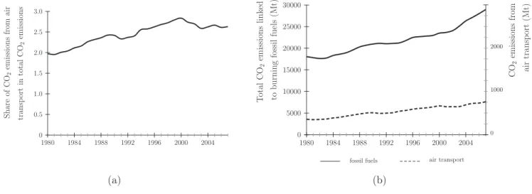
and lead to either absolute or even relative CO2 emissions reductions. As shown in Figure

1, the share of CO2 emissions coming from air transport in total CO2 emissions linked to

burning fossil fuels has been increasing from 2% in 1980 to 2.5–2.7% in 2007. This evolution seems to have slowed down during the last decade (Figure 1 (a)). However, this slower pace

cannot be associated with decreasing CO₂ emissions coming from air transport, which have

been steadily increasing from 350 Mt in 1980 to 750 Mt in 2007. Instead, it is due to an even

stronger increase of the total CO2 emissions linked to burning fossil fuels (Figure 1 (b)).

0 0.5 1.0 1.5 2.0 2.5 3.0 1980 1984 1988 1992 1996 2000 2004 S h are of C O2 em is si on s fro m ai r tra n sp ort in to ta l C O2 em is si on s 0 5000 10000 15000 20000 25000 30000 1980 1984 1988 1992 1996 2000 2004 0 1000 2000 C O2 em is si on s fro m ai r tra n sp ort (M t) T ota l C O2 em is si on s li n ke d to b u rn in g fo ss il fu el s (M t)

fossil fuels air transport

(a) (b)

Figure 1: Air traffic CO2 emissions relative to total CO2 emissions linked to burning fossil

fuels (1980 – 2007).

Source: Authors, from IEA data.

As a first conclusion, and even if Figure 1 does not take into account all greenhouse gases (GHG) emissions, the current contribution of the air transport sector to climate change may be seen as quite marginal. This statement shall not be misleading, and yield to undermine the risks associated with a continuous growth of the demand for air transport in the near future.

At least for two reasons. First, Figure 1 shows only the CO2 emissions coming from air

transport. There are other GHG associated with this activity, such as H2O and NOx, which

have important climatic impacts (IPCC, 1999). Second, it is not negligible if we include the environmental risk attached to a sustained growth for the demand in air transport, which

(6)

urges to take action. This sector indeed is growing very quickly, and the share of its emissions is steadily increasing (Figure 1). Along with increasing environmental pressures, this future development of the aviation sector may be seen as problematic.

That is why policy makers are more and more concerned by the future evolution of air

transport, especially in Europe, and aim at limiting its CO2 emissions (Rothengatter, 2010,

Zhang et al., 2010). To sum up, policy makers distinguish between two kinds of measures to limit the environmental impact of the growth of air transport. The first one consists in improving the energy efficiency of aircrafts (and thus to lower their carbon intensity) by promoting technological innovation. The second one consists in binding measures dealing with the demand for air transport. There is a sharp debate today on the best course of action to reduce significantly, and within a reasonable time horizon, GHG emissions in the air transport sector. Will technological changes be sufficient to outweigh growth in fuel use? In other words, shall we solely aim at reducing the carbon intensity of the air transport sector through innovation? Or shall we admit that technological innovation alone does not allow to achieve the objectives of stabilization and reduction of GHG that were set? In both cases, shall we limit the development of the air transport sector?

To deal with these issues, this article takes the paper by Chèze et al. (2011a) one step

further by providing original projections of CO2 emissions in the air transport sector deduced

from their forecasts of jet fuel demands. These forecasts are performed based on various scenarios of evolution of the energy efficiency of aircrafts (and others). It allows to examine more especially whether only technological innovation is able to effectively reduce the impact of air traffic on the growth of GHG. Evaluating whether the industrial policy proposed by the aviation industry will be enough to stabilize GHG emissions constitutes an important step to guide decision making in the public policy process. At the European level, such an evaluation is a pre-requisite to develop a coherent environmental policy in terms of reducing GHG emissions. If the current policies do not appear as sufficient, then additional binding measures such as the inclusion of the air transport sector in the European Union Emission Trading Scheme (EU ETS) since january 2012 would appear well-founded, despite the claims by the aeronautical industry.

The analysis proceeds in two parts. Section 2 details our benchmark scenario, along with a sensitivity analysis based on eight alternative scenarios. According to our benchmark

sce-nario, air traffic CO₂ emissions should rise at a mean yearly growth rate of 1.9%, whereas

air traffic should sharply increase (4.7%/year). Besides, none of the scenarios anticipates a

decrease, or even a stabilization, of CO2 emissions in the air transport sector by 2025

(7)

the results obtained with (i) the projections obtained in the academic literature and by the aeronautical sector, and (ii) the SRES scenarios by the IPCC (Nakicenovic and Swart, 2000; IPCC, 2007a, 2007b). Finally, Section 4 concludes.

2 World and regional air traffic CO

2

emissions projections

until 2025: Benchmark scenario and sensitivity analysis

This Section presents various projections of CO2 emissions coming from air transport by 2025.

These forecasts are deduced from the preliminary forecasts of jet fuel demand presented in Chèze et al. (2011a). This modeling, and the associated forecasts, are applied to eight geographical zones and at the world level (i.e. the sum of the eight regions). Air traffic forecasts are computed for the following regions: Central and North America, Latin America, Europe, Russia and Commonwealth of Independent States (CIS), Africa, the Middle East, Asian countries and Oceania (except China). The eighth region is China, in order to have a specific focus on this country. By doing so, we propose an analysis of potential future trends

of air transport in terms of CO2 emissions, both at the world and regional levels. Note that

a simpler analysis of the future yearly mean growth rates of world air traffic emissions may mask a wide heterogeneity between geographical zones.

Theses results mostly depend on two broad hypotheses. The first one concerns the future evolution of economic activity in the various regions (estimated from regional Gross Domestic Product (GDP) indicators). The second hypothesis deals with the energy efficiency coeffi-cients that have been chosen to conduct the analysis, as well as their evolution overtime (i.e. energy efficiency gains). Section 2.1 summarizes these hypotheses and the air traffic forecasts obtained. Section 2.2 presents our scenarios for the future evolution of air traffic in terms of

CO2 emissions. Section 2.3 investigates how much improvement in energy efficiency is needed

to stabilize the CO2 emissions coming from air transport.

2.1 Forecasting air transport demand and traffic efficiency

improve-ments until 2025 . . .

The methodology used can be summarized as follows (see Chèze et al., 2010 for more details).

(8)

jet fuel consumed1_{. As jet fuel is only used as a fuel in the aviation sector, its consumption}

depends very closely on the demand for mobility for this transportation means, which needs to be first analysed.

Air traffic projections are estimated by using econometric methods based on the historical relationship between air traffic and its main drivers: GDP growth, jet fuel prices and exoge-neous shocks (Chèze et al., 2010). GDP appears to have a positive influence on air traffic, whereas the influence of the jet fuel price – above a given threshold – is negative. Exogenous shocks may also have a (negative) impact on air traffic growth rates. The sensitivity of air transport demand depends on the degree of maturity of the market in the region consid-ered. To account for this effect, the econometric modeling is carried out by using dynamic

panel-data models for the eight geographical zones2_.

Based on assumptions on the evolution of the main drivers, we obtain different air traffic forecasts scenarios which rely on a crucial assumption: the future evolution of the eight geographical regions’ GDP growth rates. Our Baseline air traffic forecast scenario, i.e. the “IMF GDP growth rates” scenario (see Figure 2), relies in particular on the International Monetary Fund (IMF) previsions of these GDP growth rates until 2014. According to this scenario, world air traffic should, overall, increase at a yearly mean growth rate of 4.7%

between 2008 and 2025, rising from 637.4 to 1391.8 billion Revenue Tonne-Kilometre (RTK)3

(see also Table 1). These air traffic forecasts differ from one region to another. At the regional level, RTK yearly average growth rates range from 3% per year in Central and North America to 8.2% per year in China (Table 1, first two columns). Two other air traffic forecast scenarios are defined to measure the sensitivity of air traffic to changes in GDP growth rates: (i) in the “Low GDP growth rates” air traffic forecasts scenario, the IMF GDP growth rates are decreased by 10%, (ii) in the “High GDP growth rates” air traffic forecasts scenario, the IMF GDP growth rates are increased by 10% (see also Figure 2).

Once obtained, forecasts of air transport have to be converted into corresponding quantities

of CO2 emissions. This task is performed based on the specific ‘Traffic Efficiency method’

developed by the UK DTI (Department of Trade and Industry) for the special IPCC report on air traffic (IPCC, 1999). The idea underlying this method is that the growth of jet fuel

1

Once completely oxydized, one kilogram of jet fuel (Jet-A1 or Jet-A) consumed emits 3.156 kilograms of

CO2. Note that this emissions factor is officially used by the European Commission to account for the CO2

emissions from the aviation sector towards its inclusion in the EU ETS by 2012 (see Amendment C(2009) 2887 completing the Directive 2009/339/CE and the Decision 2007/589/CE).

2

The influence of the main air traffic drivers is estimated by using the Arellano-Bond estimator.

3

Revenue Tonne-Kilometre is defined as one tonne of load (passengers and/or cargo) carried for one kilo-metre.

(9)

demand following the growth of air traffic is mitigated by energy efficiency gains. Energy efficiency improvements are obtained thanks to enhancements of (i) Air Traffic Management (ATM), (ii) existing aircrafts (changes in engines for example) and (iii) the production of more

efficient aircrafts (which is linked to the rate of change of aircrafts)4_{. Besides, by improving}

their load factors, airlines hold a relatively easy way to diminish their jet fuel consumption,

and thus their CO2 emissions, without achieving any technological progress.

The conversion of air traffic forecasts into jet fuel is based on the ‘Traffic Efficiency im-provement’ hypothesis, which relies on two crucial assumptions concerning the evolution of (i) weight load factors (WLF) and (ii) energy efficiency coefficients. The former assumption has

a marginal effect compared to the latter one5_{. To determine both energy efficiency coefficients}

and their expected growth rates – corresponding to energy efficiency gains – we do not choose

to use the common approach and the results based on manufacturers’ information6 _{but an}

alternative one. As explained in Chèze et al. (2011b), we compare the evolution of each regional fleet’s jet fuel consumption (taken from IEA data) and air traffic (taken from ICAO data) to compute directly the energy efficiency coefficients of regional aircraft fleets and their corresponding energy efficiency gains.

Our approach highlights the following results on [air traffic] energy [efficiency] gains: (i) some regional fleets are more energy efficient than others, and (ii) they do not encounter the same energy gains. These results yield us to define the following three “Traffic efficiency improvements” scenarios based on the “energy efficiency gains” scenarios:

• “Heterogeneous energy gains’: this scenario aims at reflecting the heterogeneity of energy gains observed among regions during the past. Globally, this scenario defines the future energy gains of a given region as corresponding to the energy gains recorded during the

period 1996-20087_.

• “Low energy gains’: the “Heterogeneous energy gains” hypotheses are decreased by 10%. • “High energy gains’: the “Heterogeneous energy gains” hypotheses are increased by 10%.

4

See among others on this topic Greene (1992, 1996, 2004), IPCC (1999), Lee et al. (2001, 2004, 2009), Eyers et al. (2004), Lee (2010).

5

For the interested reader, we provide more details concerning the assumptions on the evolution of energy efficiency coefficients in what follows. Regarding the evolution of each region’s WLF, it is assumed that, when positive, the WLF yearly mean growth rate of the period 1983-2006 is applied until the region’s WLF reaches the 75% value. Otherwise, the WLF yearly mean growth rate of the period 1996-2006 is applied until it reaches the 75% value.

6

For illustrations of the common approach, see Greene (1992, 1996, 2004), IPCC (1999), and Eyers et al. (2004).

7

(10)

2.2 . . . and corresponding aviation CO

2

emissions

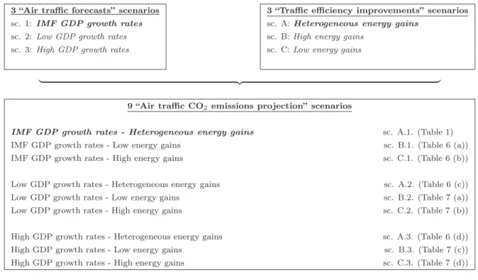
Section 2.1 has presented three “air traffic forecasts” scenarios and three “traffic efficiency

improvements” scenarios. By combining these scenarios, we obtain nine “Air traffic CO2

emissions projection” scenarios, as summarized in Figure 2.

3 “Air traffic forecasts” scenarios 3 “Traffic efficiency improvements” scenarios

sc. 1: IMF GDP growth rates sc. A: Heterogeneous energy gains

sc. 2: Low GDP growth rates sc. B: High energy gains

sc. 3: High GDP growth rates sc. C: Low energy gains

| {z }

9 “Air traffic CO2 emissions projection” scenarios

IMF GDP growth rates - Heterogeneous energy gains sc. A.1. (Table 1)

IMF GDP growth rates - Low energy gains sc. B.1. (Table 6 (a))

IMF GDP growth rates - High energy gains sc. C.1. (Table 6 (b))

Low GDP growth rates - Heterogeneous energy gains sc. A.2. (Table 6 (c))

Low GDP growth rates - Low energy gains sc. B.2. (Table 7 (a))

Low GDP growth rates - High energy gains sc. C.2. (Table 7 (b))

High GDP growth rates - Heterogeneous energy gains sc. A.3. (Table 6 (d))

High GDP growth rates - Low energy gains sc. B.3. (Table 7 (c))

High GDP growth rates - High energy gains sc. C.3. (Table 7 (d))

Figure 2: The nine “Air traffic CO2 emissions projection” scenarios.

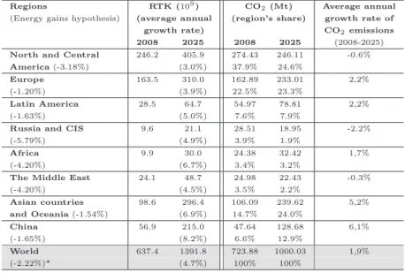
Our benchmark scenario relies on the hypotheses coming from the “IMF GDP growth rates” scenario of evolution of air traffic, and from the “Heterogeneous energy gains” scenario of evolution of traffic efficiency improvement (sc. A.1., see Figure 2). Table 1 contains the

forecasts of CO2 emissions obtained with this scenario for the eight regions and the world.

According to the benchmark scenario, the CO2 emissions coming from air transport should

rise from 725 Mt in 2008 to nearly 1,000 Mt in 2025 at the world level, i.e. an increase by 38% (1.9% per year on average) in less than two decades. This increase is due to the growth of air traffic by 4.7% per year on average on the one hand, and to the hypothesis of increasing the energy efficiency of the aircraft fleet by 2.2% per year on the other hand. These projections of air traffic are globally in line with previous literature (Airbus, 2007; Boeing, 2009). The hypothesis concerning the evolution of energy efficiency (2.2% per year, i.e. an improvement

of 32% between 2008 and 20258_{) is globally higher than the values found typically in the}

8

This percentage expressed in absolute value corresponds to -2.2%/year cumulated over seventeen years. A negative growth rate corresponds to a gain (and not a decrease) in energy efficiency.

(11)

Regions RTK (109

) CO2(Mt) Average annual

(Energy gains hypothesis) (average annual (region’s share) growth rate of growth rate) CO2emissions

2008 2025 2008 2025 (2008-2025) North and Central 246.2 405.9 274.43 246.11 -0.6% America (-3.18%) (3.0%) 37.9% 24.6%

Europe 163.5 310.0 162.89 233.01 2,2%

(-1.20%) (3.9%) 22.5% 23.3%

Latin America 28.5 64.7 54.97 78.81 2,2%

(-1.63%) (5.0%) 7.6% 7.9%

Russia and CIS 9.6 21.1 28.51 18.95 -2.2%

(-5.79%) (4.9%) 3.9% 1.9%

Africa 9.9 30.0 24.38 32.42 1,7%

(-4.20%) (6.7%) 3.4% 3.2%

The Middle East 24.1 48.7 24.98 22.43 -0.3%

(-4.20%) (4.5%) 3.5% 2.2% Asian countries 98.6 296.4 106.09 239.62 5,2% and Oceania (-1.54%) (6.9%) 14.7% 24.0% China 56.9 215.0 47.64 128.68 6,1% (-1.65%) (8.2%) 6.6% 12.9% World 637.4 1391.8 723.88 1000.03 1,9% (-2.22%)* (4.7%) 100% 100% Notes:

- The first column presents 2008 and 2025 air traffic forecasts expressed in RTK (for more details, see Section 2.1). Figures into brackets represent yearly mean growth rate of air traffic forecasts between 2008 and 2025.

- The other two columns concern air traffic CO2projections.

The second column presents 2008 and 2025 CO2 emissions forecasts expressed in million tonnes (Mt). For each geographical

region, CO2emissions projections are computed from jet fuel forecasts by using a factor of 3.156. Jet fuel forecasts are computed

from air traffic ones according to assumptions made on traffic efficiency improvements (for more details, see Section ??). In the

second column, figures expressed in % terms indicate the share of each region’s CO2 emissions in 2008 and 2025.

Finally, the third column indicates the % yearly mean growth rate of CO2emissions projections between 2008 and 2025.

* This figure corresponds to the world level energy gains (per year until 2025) resulting from regional energy gains hypothesis as defined in the ‘Heterogeneous energy gains’ traffic efficiency improvements scenario.

Table 1: Air traffic and corresponding CO2 emissions projections for the years 2008 and 2025

– Benchmark scenario.

literature9_.

Our benchmark scenario therefore anticipates a strong growth of CO2 emissions coming

from air transport, even if it relies on optimistic assumptions of energy efficiency improvements

for the aircraft fleet. This evolution implies a deep transformation of the repartition of CO2

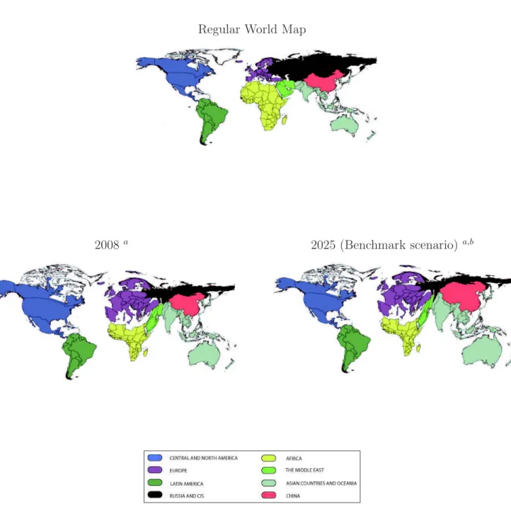
emissions between regions from 2008 to 2025. Table 1 shows that the growth potential of air traffic lies in Asia and China, with an increase comprised between 6.9% and 8.2% per year on

average10_{. Hence, the CO}

2 emissions coming from Asia and China would represent almost a

third of the total CO2 emissions coming from the air transport sector by 2025. North America

and Europe would still remain the geographic zones predominantly emitting GHG, but the

9

Currently, the values typically found in the literature are comprised between 1.5%/year (Lee et al., 2004) and 2.2%/year (Airbus, 2007, 2009). See Eyers et al. (2004) and Mayor and Tol (2010) for a literature review.

10

(12)

share of these two regions would for the first time be inferior to 50%. Figure 3 illustrates

these comments by proposing an alternative view of the share of each region’s CO2 emissions

in 2008 and 2025. These expected changes in the structure of repartition of emissions in the air transport sector highlight that it would be very difficult to decrease the level of global aviation emissions, at least in the medium term. Effectively, it is more costly (in terms of GDP points) to reduce GHG emissions in emerging countries (with high growth rates) compared to developed countries (Quinet, 2009).

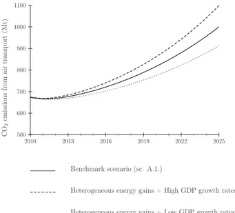
To evaluate the robustness of these results, we run a sensitivity analysis. For the bench-mark scenario, we focus on (i) the evolution of economic growth assumptions, and (ii) the assumptions regarding the energy efficiency improvements of the aircraft fleet. Forecasts of the eight alternative scenarios compared to the benchmark scenario are shown in Tables 6 to 7 (see the Appendix). Figure 4 summarizes the results of four alternative scenarios, along with the benchmark scenario. Graph (a) shows the sensitivity of these results to the assumptions

on energy efficiency improvements. CO2 emissions forecasts at the world level depend on

decreases (Table 6.a and Figure 4, gray dashed curve) or increases (Table 6.b and Figure 4, black dashed curve) by 10% of the energy efficiency of the regional aircraft fleets compared to the benchmark scenario (Table 1 and Figure 4, bold curve). Graph (b) shows the sensitivity

of these results to the assumptions on GDP forecasts. CO2 emissions forecasts at the world

level depend on decreases (Table 6.c and Figure 4, gray dashed curve) or increases (Table 6.d and Figure 4, black dashed curve) by 10% of the level of expected economic activity compared to the benchmark scenario (Table 1 and Figure 4, bold curve).

According to Figure 4.a, a decrease (an increase) by 10% of the assumptions on energy ef-ficiency improvements compared to the benchmark scenario yields to an increase (a decrease)

of CO2 emissions coming from air transport by 4.2% (4%) in 2025 (see Tables 1, 6.a and

6.b). According to Figure 4.b, a decrease (an increase) by 10% of the assumptions on the expected level of economic activity compared to the benchmark scenario yields to a decrease

(an increase) of CO2 emissions coming from air transport by 8.8% (9.8%) in 2025 (see Tables

1, 6.c and 7.b). Ceteris paribus, CO2 emissions coming from air transport seem to be more

sensitive to the variation of economic activity than to the variation of energy efficiency im-provements. Moreover, by comparing the forecasts of these nine scenarios, we observe that

the CO₂ emissions coming from air transport should rise between 22% (Table 7.b) and 57%

(Table 7.c) at the world level.

None of the scenarios considered yields to a decrease, or even a stabilization, of the level of emissions by 2025. This result is obtained despite the introduction of strong hypotheses on energy efficiency gains in the air transport sector. Therefore, the improvement in energy

(13)

Regular World Map

2008 a _{2025 (Benchmark scenario)} a,b

Notes:

a

These cartograms size the geographical zones according to their relative weight in world CO2 emissions

(expressed in Mt), offering an alternative view to a regular map of their projected evolution from 2008 to 2025. Maps generated using ScapeToad.

b

Projections realized according to the “IMF GDP growth rates” air traffic forecasts scenario combined with the “Heterogeneous energy gains” traffic efficiency improvements scenario, i.e. the “Benchmark ” Air traffic CO2 emissions projection scenario (sc. A.1., as synthesized in Figure 2).

Figure 3: An alternative view of the projected evolution of the share of each region’s CO₂

(14)

500 600 700 800 900 1000 1100 2010 2013 2016 2019 2022 2025 C O2 em is si on s fro m ai r tra n sp ort (M t) 500 600 700 800 900 1000 1100 2010 2013 2016 2019 2022 2025 C O2 em is si on s fro m ai r tra n sp ort (M t)

IMF GDP growth rates + Low energy gains (sc. B.1.) IMF GDP growth rates + High energy gains (sc. C.1.) Benchmark scenario (sc. A.1.)

Heterogeneous energy gains + Low GDP growth rates (sc. A.2.) Heterogeneous energy gains + High GDP growth rates (sc. A.3.) Benchmark scenario (sc. A.1.)

(a) Sensitivity to the assumptions on energy effi-ciency improvements.

(b) Sensitivity to the assumptions on GDP fore-casts.

Figure 4: Sensitivity analysis of aviation CO2 emissions projections.

efficiency alone does not appear to be sufficient to compensate for the increase in air traffic and its negative environmental consequences.

2.3 How much improvement in energy efficiency is needed to

stabi-lize the CO

2

emissions coming from air transport?

Let us investigate here the hypothetical case where the increase in the energy efficiency of the

aircraft fleet would stabilize (at the current levels of 700 Mt) the air transport CO₂ emissions

by 2025. The results of this scenario are shown in Table 2.

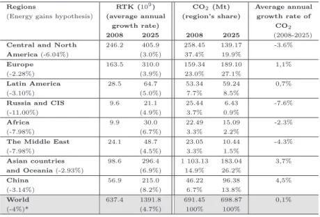
To stabilize CO2 emissions without constraining the demand for air transport, our results

suggest that energy efficiency should be improved by 4% per year on average for the world aircraft fleet, i.e. an increase by 50% in seventeen years. This result implies that the hypothesis on energy efficiency improvements should be multiplied by two compared to our (already optimistic at 2.2% per year, see Table 1) benchmark scenario. A the time of writing, and given the current technological standards, such a high level of improvement seems unrealistic.

Without limits on the demand for air transport, it appears therefore that CO2 emissions will

increase significantly, unless major economic and/or exogenous shocks (such as the sub-prime crisis or the 9/11 terrorist attacks) occur during the period. Besides, we have shown earlier

(15)

to energy efficiency improvements.

Regions RTK (109

(Energy gains hypothesis) (average annual (region’s share) growth rate of

growth rate) CO2

2008 2025 2008 2025 (2008-2025) Central and North 246.2 405.9 258.45 139.17 -3.6% America (-6.04%) (3.0%) 37.4% 19.9%

Europe 163.5 310.0 159.34 189.10 1,1%

(-2.28%) (3.9%) 23.0% 27.1%

Latin America 28.5 64.7 53.34 59.24 0,7%

(-3.10%) (5.0%) 7.7% 8.5%

Russia and CIS 9.6 21.1 25.44 6.43 -7.6%

(-11.00%) (4.9%) 3.7% 0.9%

Africa 9.9 30.0 22.49 15.09 -2.3%

(-7.98%) (6.7%) 3.3% 2.2%

The Middle East 24.1 48.7 23.05 10.44 -4.3%

(-7.98%) (4.5%) 3.3% 1.5% Asian countries 98.6 296.4 1 103.13 183.04 3,7% and Oceania (-2.93%) (6.9%) 14.9% 26.2% China 56.9 215.0 46.22 96.38 4,5% (-3.14%) (8.2%) 6.7% 13.8% World 637.4 1391.8 691.45 698.87 0,1% (-4%)* (4.7%) 100% 100% Notes:

* This figure corresponds to the world level energy gains (per year until 2025) resulting from regional energy gains hypothesis.

Table 2: Air traffic and CO₂ emissions forecasts for the years 2008 and 2025 - Hypothetical

case where the increase in the energy efficiency of the aircraft fleet would stabilize the air

transport CO2 emissions by 2025.

3 Comparing our estimates with previous literature and

the SRES scenarios from the IPCC

This Section compares the results obtained in this article with previous literature. We compare

first our CO2 emissions forecasts in the air transport sector with the estimates found in other

studies, before confronting them to the SRES scenarios by the IPCC (Nakicenovic and Swart, 2000; IPCC, 2007a, 2007b). Note that previous studies differ in terms of hypotheses, which makes difficult the direct comparison with our estimates. The comparison with the IPCC SRES scenarios is detailed in Section 3.2.

(16)

3.1 Comparison with other CO

2

emissions forecasts from air

trans-port

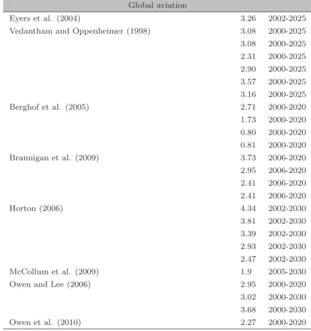
Table 3 summarizes the growth rates of CO2 emissions coming from air transport found in

previous studies. These results show that CO2 emissions could rise from 0.8% to 4% per year

during the next decade. The main differences between these forecasts are due to the under-lying model assumptions (economic growth rate, energy efficiency improvement, etc.) and to

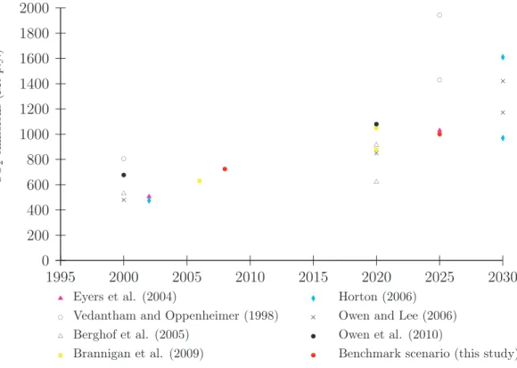
various geographical scopes. Figure 5 shows how these CO2 emissions from air transport are

forecast by a number of studies and for many scenarios11_{. Note that our forecasts are lower}

than many of other forecasts.

Global aviation

Eyers et al. (2004) 3.26 2002-2025

Vedantham and Oppenheimer (1998) 3.08 2000-2025

3.08 2000-2025 2.31 2000-2025 2.90 2000-2025 3.57 2000-2025 3.16 2000-2025 Berghof et al. (2005) 2.71 2000-2020 1.73 2000-2020 0.80 2000-2020 0.81 2000-2020 Brannigan et al. (2009) 3.73 2006-2020 2.95 2006-2020 2.41 2006-2020 2.41 2006-2020 Horton (2006) 4.34 2002-2030 3.81 2002-2030 3.39 2002-2030 2.93 2002-2030 2.47 2002-2030 McCollum et al. (2009) 1.9 2005-2030

Owen and Lee (2006) 2.95 2000-2020

3.02 2000-2030

3.68 2000-2030

Owen et al. (2010) 2.27 2000-2020

Table 3: Annual growth rates of global aviation carbon dioxide emissions - Literature review The assumptions regarding the GDP growth rate and energy efficiency improvements

are the main determinants of the CO₂ emissions forecasts. Besides, various scenarios

co-11

Gudmundsson and Anger (2012) summarize the aviation CO2 emissions studies of the IPCC IS92 and

Special Report on Emissions Scenarios storylines, where GDP growth assumptions contribute to forecast

(17)

exist. Mayor and Tol (2010) consider that CO₂ emissions linked to international tourism are dependent on income rise, and that they must therefore increase (by a factor of twelve between 2005 and 2100 according to their baseline scenario). Macintosh and Wallace (2009) hypothesize that the increase in the demand for air transport cannot be compensated by

energy efficiency improvements. Therefore, they estimate that CO2 emissions coming from

air transport will increase by 110 % during 2005-2025 at the world level. Olsthoorn (2001)

concludes that CO₂ emissions coming from air transport will be in 2020 higher by 55% to

105% compared to baseline emissions in 2000. Vedantham and Oppenheimer (1998), Eyers et al. (2004), Berghof et al. (2005), Brannigan et al. (2009), Horton (2006), McCollum et al.

(2009), Owen and Lee (2006) and Owen et al. (2010) also propose CO2 emissions forecasts

coming from air transport. Depending on the period under consideration, the underlying

assumptions and the scenario adopted, these studies show that the CO2 emissions coming from

air transport should rise at a yearly mean growth rate comprised between 0.81% (Berghof et al., 2005) and 4.34 % (Horton, 2006) during the next twenty years at the world level. According

to Vedantham and Oppenheimer (1998), the yearly mean growth rate of CO2 emissions in

the air transport sector should be in the interval [2.31%;3.57%] (i.e. between 1,430 Mt and

1,943 Mt) until 2025. Eyers et al. (2004) estimate that the CO2 emissions coming from air

transport will be multiplied by a factor of two between 2002 and 2025 to reach 1,029 Mt per

year. Berghof et al. (2005) estimate that CO₂ emissions should be multiplied by a factor

comprised between 1.2 and 1.9 during 2000-2020 to reach 880 Mt-1,049 Mt. Horton (2006)

estimates that CO2 emissions from air transport should be in the range of 970 Mt to 1,609

Mt (from a baseline of 489 Mt in 2002). Brannigan et al. (2009) estimate that CO2 emissions

from air transport will increase by 2.41% to 3.73% per year during 2006-2020 (i.e. 879 Mt to

1,048 Mt CO2 per year in 2020). Owen and Lee (2006) estimate that CO2 emissions from air

transport will be comprised between 1,172 Mt and 1,420 Mt by 2030, i.e. an increase by 3.02%

to 3.68% per year during 2000-2030. Owen et al. (2010) estimate the CO2 emissions should

be multiplied by a factor of 1.5 during 2000-2020, and by 2-3.6 during 2000-2050. Finally,

McCollum et al. (2009) anticipate that CO2 emissions from air transport will be multiplied

by a factor of two during 2005-2030.

The forecasts of CO2 emissions from air transport based on our benchmark scenario are in

the lower range compared to previous estimates. Namely, we have more optimistic assump-tions regarding the improvements in energy efficiency compared to other studies. Besides, our forecasts take into account the global economic downturn since 2007-2008, which had an

adverse impact on air traffic and therefore CO2 emissions from 2008 to 2010 (see Figure 4),

(18)

0 200 400 600 800 1000 1200 1400 1600 1800 2000 1995 2000 2005 2010 2015 2020 2025 2030 ! " ! " ! " ! " # # # # $ $ $ $ % % % % × × × × × ! ! ! ! ! ! Eyers et al. (2004)

Vedantham and Oppenheimer (1998) Berghof et al. (2005)

Brannigan et al. (2009)

Horton (2006) Owen and Lee (2006) Owen et al. (2010)

Benchmark scenario (this study)

C O2 em is si on s (M t p .y .) Notes:

- Differences between CO₂data on past and current aviation emissions tend to come from differences in fuel

sold data sources and assumptions (Brannigan et al., 2009). - Only low and high estimates are provided.

Figure 5: Comparison of results from global aviation emissions studies, 1995-2030, Mt CO2.

The next Section compares our estimates with the IPCC SRES scenarios (Nakicenovic and Swart, 2000).

3.2 Comparisons with the SRES scenarios from Nakicenovic and

Swart (2000)

The overwhelming conclusion among previous studies is that CO2 emissions coming from

air transport are strictly anticipated to increase in the near future. Even with optimistic

assumptions on energy efficiency improvements, our benchmark scenario concludes that CO2

emissions will increase by 40% in 2025. These results suggest that the air transport sector is not currently compatible with sustainable development, at least in the mid-term. To analyze more in depth this assertion, we propose in the next Sections to compare our projections of

air transport CO2 emissions with the SRES scenarios from Nakicenovic and Swart (2000). By

doing so, we will be able to check if our projections are effectively compatible, or not, with

(19)

Before presenting our comparison, we first detail briefly below the SRES scenarios.

3.2.1 SRES scenarios from Nakicenovic and Swart (2000)

To limit global warming to 2◦_{C compared to pre-industrial levels, Nakicenovic and Swart}

(2000) have elaborated several scenarios which simulate the evolution of GHG linked to hu-man activity until 2100: the SRES scenarios, for “Special Report on Emission Scenarios”. These scenarios rely on several assumptions regarding world economic growth and population growth, the growth of developing countries, environmental quality and technology diffusion (IPCC, 2007a, 2007b).

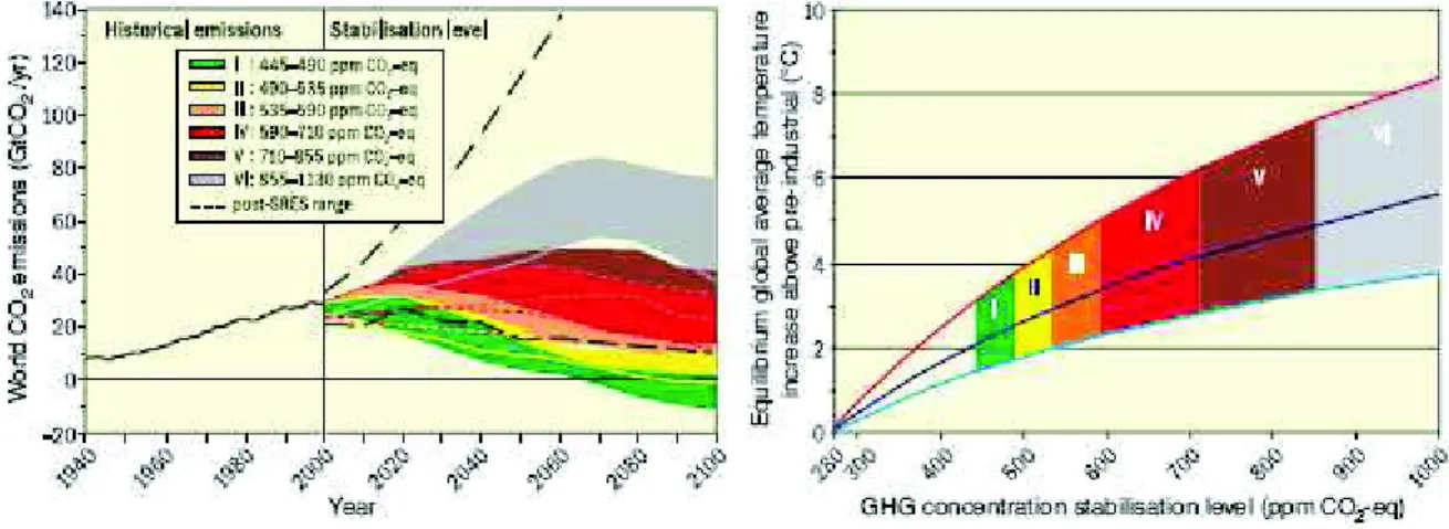
As shown in Figure 6, the maximum concentration of GHG in the atmosphere should not

exceed 450ppm in order to limit the increase in temperatures to +2◦_{C. This target implies}

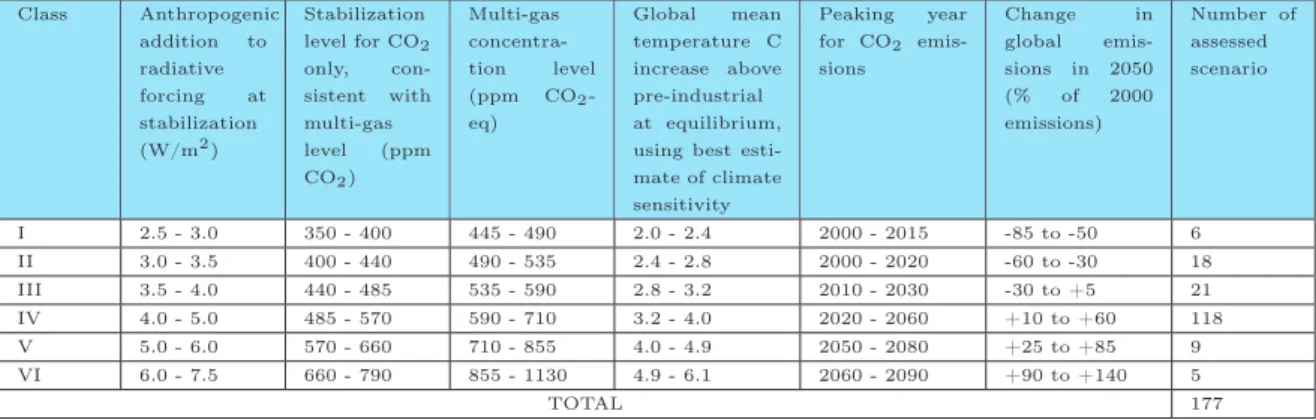
a stabilization of world emissions by 2020-2025, and a reduction by a factor of two by 2050 (in the Type I scenario). Table 4 (taken from Quinet (2009)) proposes another view of these results. In the “pessimistic” IPCC scenarios (types V and VI), global warming may be as high

as +6.1◦_{C in 2100 compared to 1900.}

Figure 6: Stabilization and equilibrium global mean temperatures.Source: IPCC (2007a).

3.2.2 Comparisons between our air traffic CO₂ emissions projections scenarios

and the IPCC ones

Table 5 compares our CO₂ emissions forecasts coming from air transport (lines, in gray) with

worldwide CO₂ emissions coming from the IPCC scenarios of type I, III, and IV12 _(columns,

12

The IPCC scenarios of type V and VI have been deliberately dismissed, as they would yield to unsustain-ably high levels of climate change.

(20)

Class Anthropogenic addition to radiative forcing at stabilization (W/m2 ) Stabilization level for CO2 only, con-sistent with multi-gas level (ppm CO2) Multi-gas concentra-tion level (ppm CO2 -eq) Global mean temperature C increase above pre-industrial at equilibrium, using best esti-mate of cliesti-mate sensitivity Peaking year for CO2 emis-sions Change in global emis-sions in 2050 (% of 2000 emissions) Number of assessed scenario I 2.5 - 3.0 350 - 400 445 - 490 2.0 - 2.4 2000 - 2015 -85 to -50 6 II 3.0 - 3.5 400 - 440 490 - 535 2.4 - 2.8 2000 - 2020 -60 to -30 18 III 3.5 - 4.0 440 - 485 535 - 590 2.8 - 3.2 2010 - 2030 -30 to +5 21 IV 4.0 - 5.0 485 - 570 590 - 710 3.2 - 4.0 2020 - 2060 +10 to +60 118 V 5.0 - 6.0 570 - 660 710 - 855 4.0 - 4.9 2050 - 2080 +25 to +85 9 VI 6.0 - 7.5 660 - 790 855 - 1130 4.9 - 6.1 2060 - 2090 +90 to +140 5 TOTAL 177

Table 4: Properties of emissions pathways for alternative CO₂ and CO₂-eq stabilization

tar-gets.

Source: Quinet (2009), from IPCC (2007a). in blue) until 2025.

Let us first detail the comparison of our benchmark scenario with the three SRES scenarios

contained in Table 5. This Table recalls the total of world CO₂ emissions, expressed in Mt, in

2008 and 2025 coming from the SRES scenarios (columns ‘Total’, in blue). Thus, for global

warming to stay within the limit of 2-2.4◦_{C in 2100 (IPCC scenario of type I), CO}

2 emissions

should be strictly inferior to 29,000 Mt in 2025 (Table 5, 1st column, 2nd row). World CO2

emissions should therefore be stable between 2008 and 2025 (Table 5, 1st column, 3rd row).

For global warming to stay within the limit of 2.8-3.2◦_{C in 2100 (IPCC scenario of type}

III), CO₂ emissions should be strictly inferior to 34,500 Mt in 2025 (Table 5, 4th column,

2nd row). World CO2 emissions should therefore increase by 19% between 2008 and 2025

(Table 5, 4th column, 3rd row). For global warming to stay within the limit of 3.2-4◦_{C in}

2100 (IPCC scenario of type III), CO2 emissions should be strictly inferior to 39,500 Mt in

2025 (Table 5, 7th column, 2nd row). World CO2 emissions should therefore increase by 36%

between 2008 and 2025 (Table 5, 7th column, 3rd row). Then, we recall our projections of

CO₂ emissions in the air transport sector coming from our ten scenarios (columns ‘Aviation’,

in gray). According to our benchmark scenario, CO2 emissions from air transport should

rise from 724 Mt in 2008 (Table 5, 2nd column, 1st row) to 1,000 Mt in 2025 (Table 5, 2nd column, 2nd row), i.e. an increase by 38% (Table 5, 2nd column, 3rd row). The comparison

between our projections and the SRES scenarios is performed by computing the share of CO2

emissions from the air transport sector in the total of world emissions in 2008 and 2025 (Table

5, column ‘Share’). For instance, the share of CO₂ emissions coming from air transport in

(21)

Table 5 indicates that, to reach the objective of limiting global warming to +2◦C _{in 2100}

as in the Type I SRES scenarios, CO2 emissions from aviation in our benchmark scenario

should represent 3.4% of world emissions in 2025 (Table 5, 3rd column, 2nd row). This would represent an increase of the share of emissions from aviation in total emissions by 38% between 2008 and 2025 (Table 5, 3rd column, 3rd row). More importantly, it reveals that this growth of emissions from aviation is not compatible with the objective of 450 ppm (Type I SRES scenarios) recommended by the IPCC (2007a, 2007b). This growth of emissions from aviation

is not compatible either with the objective of limiting global warming to +3.2◦C _{in 2100 as}

in the Type III SRES scenarios. Indeed, the share of emissions from aviation should go from 2.5% in 2008 (Table 5, 6th column, 1st row) to 2.9% in 2025 (Table 5, 6th column, 2nd row), i.e. an increase by 16% (Table 5, 6th column, 3rd row). Actually, the forecasts from our benchmark scenario are only compatible with an increase of temperatures between +3.2 and

+4◦C_{if world emissions remain on the same growth rate. The share of air transport emissions}

would effectively remain constant between 2008 and 2025 with a percentage of variation of 1% only (Table 5, 9th column, 3rd row) as shown in green.

Finally, according to Table 5, none of our nine scenarios of CO2 emissions from aviation

is compatible with the objective of limiting global warming to +3.2◦C _{(Types I to III SRES}

scenarios)13_{. Only the scenario presented in Table 2 is compatible with the objective of 450}

ppme. Again, this result is conform to our expectations, since this scenario has been explicitly

created to meet the objective by stabilizing CO2 emissions from aviation between 2008 and

2025 (see Section 2.3).

13

(22)

IPCC scenario of type I IPCC scenario of type III IPCC scenario of type IV

(445-490 ppm. i.e. 2.0-2.4o_C) _{(535-590 ppm. i.e. 2.8-3.2}o_C) _{(590-710 ppm. i.e. 3.2-4.0}o_C)

Total Aviation Share Total Aviation Share Total Aviation Share (Mt) (Mt) (%) (Mt) (Mt) (%) (Mt) (Mt) (%)

Benchmark scenario A.1. 2008 29000 724 2.5% 29000 724 2.5% 29000 724 2.5% (table 1∗) 2025 29000 1000 3.4% 34500 1000 2.9% 39500 1000 2.5% Variation 0% 38% 38% 19% 38% 16% 36% 38% 1% scenario B.1. 2008 29000 728 2.5% 29000 728 2.5% 29000 728 2.5% of table 6.a∗ ₂₀₂₅ ₂₉₀₀₀ ₁₀₄₂ _3.6% ₃₄₅₀₀ ₁₀₄₂ _3.0% ₃₉₅₀₀ ₁₀₄₂ _2.6% Variation 0% 43% 43% 19% 43% 20% 36% 43% 5% scenario C.1. 2008 29000 720 2.5% 29000 720 2.5% 29000 720 2.5% of table 6.b∗ 2025 29000 960 3.3% 34500 960 2.8% 39500 960 2.4% Variation 0% 33% 33% 19% 33% 12% 36% 33% -2% scenario A.2. 2008 29000 723 2.5% 29000 723 2.5% 29000 723 2.5% of table 6.c∗ ₂₀₂₅ ₂₉₀₀₀ ₉₁₂ _3.1% ₃₄₅₀₀ ₉₁₂ _2.6% ₃₉₅₀₀ ₉₁₂ _2.3% Variation 0% 26% 26% 19% 26% 6% 36% 26% -7% scenario A.3. 2008 29000 725 2.5% 29000 725 2.5% 29000 725 2.5% of table 6.d∗ 2025 29000 1099 3.8% 34500 1099 3.2% 39500 1099 2.8% Variation 0% 52% 52% 19% 52% 27% 36% 52% 11% scenario B.2. 2008 29000 727 2.5% 29000 727 2.5% 29000 727 2.5% of table 7.a∗ ₂₀₂₅ ₂₉₀₀₀ ₉₅₁ _3.3% ₃₄₅₀₀ ₉₅₁ _2.8% ₃₉₅₀₀ ₉₅₁ _2.4% Variation 0% 31% 31% 19% 31% 10% 36% 31% -4% scenario C.2. 2008 29000 719 2.5% 29000 719 2.5% 29000 719 2.5% of table 7.b∗ 2025 29000 875 3.0% 34500 875 2.5% 39500 875 2.2% Variation 0% 22% 22% 19% 22% 2% 36% 22% -11% scenario B.3. 2008 29000 729 2.5% 29000 729 2.5% 29000 729 2.5% of table 7.c∗ ₂₀₂₅ ₂₉₀₀₀ ₁₁₄₅ _3.9% ₃₄₅₀₀ ₁₁₄₅ _3.3% ₃₉₅₀₀ ₁₁₄₅ _2.9% Variation 0% 57% 57% 19% 57% 32% 36% 57% 15% scenario C.3. 2008 29000 721 2.5% 29000 721 2.5% 29000 721 2.5% of table 7.d∗ 2025 29000 1055 3.6% 34500 1055 3.1% 39500 1055 2.7% Variation 0% 46% 46% 19% 46% 23% 36% 46% 7% scenario 2008 29000 691 2.4% 29000 691 2.4% 29000 691 2.4% of table 2∗ ₂₀₂₅ ₂₉₀₀₀ ₆₉₉ _2.4% ₃₄₅₀₀ ₆₉₉ _2.0% ₃₉₅₀₀ ₆₉₉ _1.8% Variation 0% 1% 1% 19% 1% -15% 36% 1% -26% Notes:

- “Total” corresponds to global CO2 emissions projections for 2008 and 2025 (expressed in Mt). These projections are provided by

Nakicenovic and Swart (2000) – scenarios of type I, III and IV, as specified in columns.

- “Aviation” corresponds to our aviation CO2emissions projections for 2008 and 2025 (expressed in Mt) for a given scenario specified in

lines.

- “Share” corresponds to aviation’s share of global CO2emissions in 2008 and 2025 (expressed in %).

- A red (green) value means that this share will increase (decrease) between 2008 and 2025. Hence, a red (green) value means that scenario is not compatible (compatible) with the given IPCC scenario (type I, III or IV).

* scenarios of Tables 1, 6 and 7 are presented in Figure 2. Scenario of table 2 is a hypothetical case where the increase in the energy efficiency of the aircraft fleet would stabilize the CO2emissions coming from air transport by 2025 (see Section 2.3).

Table 5: Comparison of the study’s CO2 forecasts with those provided by IPCC (scenarios of

type I, III and IV).

(23)

4 Conclusion

CO2 emissions have grown substantially in the aviation sector over the last decades. Air

transport is the world’s fastest growing source of GHG. Aviation contributes to about 8% of

fuel consumption and between 2.5%-3% of anthropogenic CO2 emissions (IEA, 2009a, 2009b,

2009c). At present, aviation cannot be considered as a major contributor to climate change. Nevertheless, its high growth rate attracts the attention of policy makers. Addressing GHG emissions from aviation is challenging. Two types of mitigation options are distinguished: (i) technological and operational possibilities, and (ii) policy options (market-based options such as EU ETS or regulatory regimes). As it can be expected, these latter options face fierce opposition by most stakeholders in the aeronautical industry. Nevertheless, it seems that anticipated technological progress would not be sufficient to completely annihilate the

negative impact of aviation on the rise of CO2 emissions in the mid-term.

This paper contains forecasting results of world and regional aviation CO2 emissions until

2025. To do so, it relies heavily on the econometric results and traffic efficiency improvement assumptions developed in Chèze et al. (2010, 2011a, 2011b). Following an econometric analysis of the relationship between air traffic and its main drivers, air traffic forecasts are converted into quantities of jet fuel by using a methodology which allows obtaining energy efficiency coefficients without prior assumptions on the composition of the aircraft fleet. This

paper goes one step further by presenting original air traffic CO2 emissions deduced from

the latter forecasts. The projections of aviation CO2 emissions are provided for eight regions

and at the world level (i.e. the sum of the eight regions). Nine scenarios of air traffic CO₂

emissions projections are proposed. Depending on the scenario under consideration, the CO2

emissions coming from air traffic are projected to increase, at the world level, with yearly mean growth rates comprised between 1.2% (sc. C.2.) and 2.7% (sc. B.3.) from 2008 to

2025. Our Benchmark scenario (sc. A.1.) anticipates an increase of air traffic CO2 emissions

of about 2% per year at the world level (i.e. about 38% in less than two decades), from 725

Mt of CO₂ in 2008 to nearly 1,000 Mt in 2025, and ranging from -2.2% (Russia and CIS) to

+6.1% (China) at the regional level.

These air traffic CO2 emissions are used to investigate whether technological progress

would be sufficient to outweigh the growth in fuel use, and thus lead to CO2 emission

re-ductions. None of our nine scenarios appears compatible with the objective of 450 ppm recommended by the IPCC. None is either compatible with the IPCC scenario of type III,

which aims at limiting global warming to 3.2◦_{C compared to the pre-industrial era. Of course,}

(24)

mo-ment (recall Figure 1). Moreover, growth in the aviation sector could be compensated by disproportionally higher emission reductions in other economic sectors. From an economic viewpoint, this alternative may be justified if it has been proved that the air transport sec-tor is among the secsec-tors with the highest marginal abatement costs. This issue can not be adressed here due to our partial equilibrium analysis based on trend modeling. It is clearly a caveat to the work presented here. However, one can also argue that the current debate to

limit/reduce the CO₂ emissions coming from air transport is a political one, and not linked

to economic or efficiency arguments. At least in Europe, the inclusion of the air transport sector in the EU ETS tends to prove that policy makers are willing to anihilate, or at least

reduce, the CO2 emissions coming from this sector. It appears crucial to understand whether

a constrained level of CO2 emissions would lead to technological progress, or to a decreasing

use of air travel. Both outcomes would not have the same impacts on the stakeholders of the aeronautical sector. According to our results, if the aviation sector continues to be one of the fastest growing sectors of the global economy, technological progress should not be sufficient

to completely annihilate its impact on the rise of anthropogenic CO2 emissions. Indeed, CO2

emissions from aviation are unlikely to diminish unless there is a radical shift in technology14

and/or travel demand is restricted. Such a growth in the aviation sector cannot be then con-sidered to be in line with global climate policy. Despite aircraft manufacturers’ and airlines’

initiatives, the control of CO₂ emissions from aviation should require more binding measures

from policy makers. From this perspective, the inclusion of the aviation sector in the EU ETS appears to go one step further towards “sustainable aviation”.

14

(25)

5 Appendix

Regions RTK (109₎ _CO

2(Mt) Average annual Regions RTK (109) CO2(Mt) Average annual

(Energy gains hypothesis) (average annual (region’s share) growth rate of (Energy gains hypothesis) (average annual (region’s share) growth rate of

growth rate) CO2 growth rate) CO2

2008 2025 2008 2025 (2008-2025) 2008 2025 2008 2025 (2008-2025)

North and Central 246.2 405.9 276.24 261.93 -0.3% North and Central 246.2 405.9 272.63 231.20 -1.0 %

America (-2.86%) (3.0%) 38.0% 25.1% America (-3.50%) (3.0%) 37.9 % 24.1 %

Europe 163.5 310.0 163.28 238.45 2,3% Europa 163.5 310.0 162.49 227.69 2,1 %

(-1.08%) (3.9%) 22.4% 22.9% (-1.32%) (3.9%) 22.6 % 23.7 %

Latin America 28.5 64.7 55.15 81.33 2,4% Latin America 28.5 64.7 54.79 76.37 2,1 %

(-1.47%) (5.0%) 7.6% 7.8% (-1.79%) (5.0%) 7.6 % 8.0 %

Russia and CIS 9.6 21.1 28.86 21.29 -1.6% Russia and CIS 9.6 21.1 28.16 16.86 -2.8 %

(-5.21%) (4.9%) 4.0% 2.0% (-6.37%) (4.9%) 3.9 % 1.8 %

Africa 9.9 30.0 24.59 35.23 2,1% Africa 9.9 30.0 24.17 29.82 1,3 %

(-3.78%) (6.7%) 3.4% 3.4% (-4.62%) (6.7%) 3.4 % 3.1 %

The Middle East 24.1 48.7 25.20 24.37 0,1% The Middle East 24.1 48.7 24.76 20.63 -0.8 %

(-3.78%) (4.5%) 3.5% 2.3% (-4.62%) (4.5%) 3.4 % 2.1 %

Asian countries 98.6 296.4 106.42 246.84 5,3% Asian countries 98.6 296.4 105.76 232.60 5,0 %

and Oceania (-1.39%) (6.9%) 14.6% 23.7% and Oceania (-1.69%) (6.9%) 14.7 % 24.2 %

China 56.9 215.0 47.80 132.85 6,3% China 56.9 215.0 47.48 124.64 5,9 %

(-1.49%) (8.2%) 6.6% 12.7% (-1.82%) (8.2%) 6.6 % 13.0 %

World 637.4 1391.8 727.55 1042.29 2,2% World 637.4 1391.8 720.23 959.81 1,7 %

(-2%)* (4.7%) 100% 100% (-2.4%)* (4.7%) 100% 100%

(a) scenario B.1. (b) scenario C.1.

Regions RTK (109

) CO2(Mt) Average annual Regions RTK (109

2008 2025 2008 2025 (2008-2025) 2008 2025 2008 2025 (2008-2025)

North and Central 246.1 391.2 274.32 237.23 -0.9% North and Central 246.3 421.0 274.54 255.29 -0.4%

America (-3.18%) (2.8%) 37.9% 26.0% America (-3.18%) (3.2%) 37.9% 23.2%

Europe 163.3 287.7 162.73 216.28 1,8% Europe 163.7 333.7 163.04 250.88 2.7%

(-1.20%) (3.5%) 22.5% 23.7% (-1.20%) (4.4%) 22.5% 22.8%

Latin America 28.5 62.7 54.93 76.36 2,0% Latin America 28.6 66.8 55.01 81.33 2.4%

(-1.63%) (4.8%) 7.6% 8.4% (-1.63%) (5.2%) 7.6% 7.4%

Russia and CIS 9.6 19.1 28.43 17.11 -2.8% Russia and CIS 9.6 23.4 28.58 20.97 -1.6%

(-5.79%) (4.2%) 3.9% 1.9% (-5.79%) (5.5%) 3.9% 1.9%

Africa 9.9 27.6 24.34 29.82 1,2% Africa 10.0 32.7 24.42 35.23 2,2%

(-4.20%) (6.2%) 3.4% 3.3% (-4.20%) (7.2%) 3.4% 3.2%

The Middle East 24.0 42.3 24.88 19.50 -1.1% The Middle East 24.2 56.0 25.07 25.78 0,5%

(-4.20%) (3.7%) 3.4% 2.1% (-4.20%) (5.4%) 3.5% 2.3%

Asian countries 98.3 253.8 105.77 205.17 4,2% Asian countries 98.9 345.7 106.42 279.45 6,1%

and Oceania (-1.54%) (6.0%) 14.6% 22.5% and Oceania (-1.54%) (7.9%) 14.7% 25.4%

China 56.7 184.4 47.50 110.38 5,2% China 57.1 250.3 47.79 149.82 7,0%

(-1.65%) (7.3%) 6.6% 12.1% (-1.65%) (9.2%) 6.6% 13.6%

World 636.5 1268.9 722.89 911.84 1,4% World 638.3 1529.5 724.88 1098.75 2.5%

(-2.22%)* (4.2%) 100% 100% (-2.22%)* (5.3%) 100% 100%

(c) scenario A.2. (d) scenario A.3.

Notes:

Table 6: Air traffic and corresponding CO₂ emissions projections for the years 2008 and 2025

(26)

Regions RTK (109₎ _CO

2(Mt) Average annual Regions RTK (109) CO2(Mt) Average annual

2008 2025 2008 2025 (2008-2025) 2008 2025 2008 2025 (2008-2025)

America (-2.86%) (2.8%) 38.0% 26.6% America (-3.50%) (2.8%) 37.9% 25.5%

Europe 163.3 287.7 163.12 221.32 1,9% Europe 163.3 287.7 162.33 211.34 1,6%

(-1.08%) (3.5%) 22.5% 23.3% (-1.32%) (3.5%) 22.6% 24.2%

Latin America 28.5 62.7 55.11 78.80 2,2% Latin America 28.5 62.7 54.75 73.99 1,9%

(-1.47%) (4.8%) 7.6% 8.3% (-1.79%) (4.8%) 7.6% 8.5%

(-5.21%) (4.2%) 4.0% 2.0% (-6.37%) (4.2%) 3.9% 1.7%

Africa 9.9 27.6 24.55 32.40 1,7% Africa 9.9 27.6 24.12 27.43 0,8%

(-3.78%) (6.2%) 3.4% 3.4% (-4.62%) (6.2%) 3.4% 3.1%

The Middle East 24.0 42.3 25.10 21.18 -0.7% The Middle East 24.0 42.3 24.66 17.93 -1.6%

(-3.78%) (3.7%) 3.5% 2.2% (-4.62%) (3.7%) 3.4% 2.0%

Asian countries 98.3 253.8 106.10 211.35 4,4% Asian countries 98.3 253.8 105.44 199.16 4.0%

China 56.7 184.4 47.66 113.95 5,3% China 56.7 184.4 47.34 106.91 5.0%

(-1.49%) (7.3%) 6.6% 12.0% (-1.82%) (7.3%) 6.6% 12.2%

World 636.5 1268.9 726.54 950.72 1.6% World 636.5 1268.9 719.24 874.84 1.2%

(-2%)* (4.2%) 100% 100% (-2.4%)* (4.2%) 100% 100%

(a) scenario B.2. (b) scenario C.2.

Regions RTK (109

) CO2(Mt) Average annual Regions RTK (109

2008 2025 2008 2025 (2008-2025) 2008 2025 2008 2025 (2008-2025)

America (-2.86%) (3.2%) 37.9% 23.7% America (-3.50%) (3.2%) 37.8% 22.7%

Europe 163.7 333.7 163.44 256.73 2,8% Europe 163.7 333.7 162.65 245.15 2.6%

(-1.08%) (4.4%) 22.4% 22.4% (-1.32%) (4.4%) 22.6% 23.2%

Latin America 28.6 66.8 55.19 83.93 2,6% Latin America 28.6 66.8 54.83 78.81 2.2%

(-1.47%) (5.2%) 7.6% 7.3% (-1.79%) (5.2%) 7.6% 7.5%

(-5.21%) (5.5%) 4.0% 2.1% (-6.37%) (5.5%) 3.9% 1.8%

Africa 10.0 32.7 24.64 38.28 2,6% Africa 10.0 32.7 24.21 32.41 1.7%

(-3.78%) (7.2%) 3.4% 3.3% (-4.62%) (7.2%) 3.4% 3.1%

The Middle East 24.2 56.0 25.29 28.01 0,9% The Middle East 24.2 56.0 24.85 23.71 -0.0%

(-3.78%) (5.4%) 3.5% 2.4% (-4.62%) (5.4%) 3.4% 2.2%

Asian countries 98.9 345.7 106.75 287.87 6,3% Asian countries 98.9 345.7 106.08 271.26 5.9%

China 57.1 250.3 47.95 154.67 7,2% China 57.1 250.3 47.63 145.12 6,9% (-1.49%) (9.2%) 6.6% 13.5% (-1.82%) (9.2%) 6.6% 13.8% World 638.3 1529.5 728.54 1144.76 2.7% World 638.3 1529.5 721.22 1054.93 2.3% (-2%)* (5.3%) 100% 100% (-2.4%)* (5.3%) 100% 100% (c) scenario B.3. (d) scenario C.3. Notes:

Table 7: Air traffic and corresponding CO₂ emissions projections for the years 2008 and 2025

(27)

References

Airbus, 2007. Flying by Nature: Global Market Forecast 2007-2026. Airbus, France. Airbus, 2009. Flying by Nature: Global Market Forecast 2009-2028. Airbus, France. Berghof, R., Schmitt, A., Eyers, C., Haag, K., Middel, J., Hepting, M., 2005. Constrained Scenarios on Aviation and Emissions. CONSAVE 2050 Final Report Project, Germany.

Boeing, 2009. Current Market Outlook 2009-2028. Boeing, USA.

Brannigan, C., Paschos, V., Eyers, C., Wood, J., 2009. Report on International Aviation and Maritime Emissions in a Copenhagen (post 2012) Agreement. AEA and QINETIQ. Report to the UK Department for Transport, June, UK.

Chèze, B., Gastineau, P., Chevallier, J., 2010. Forecasting Air Traffic and Corresponding Jet-Fuel Demand until 2025. Les cahiers de l’économie, Série Recherche, 77, IFP School.

Chèze, B., Gastineau, P., Chevallier, J., 2011a. Forecasting world and regional aviation jet fuel demands to the mid-term (2025). Energy Policy, 39(9), 5147-5158.

Chèze, B., Gastineau, P., Chevallier, J., 2011b. Air traffic energy efficiency differs from place to place: new results from a macro-level approach. International Economics, 126-127, 31-58.

Eyers, C., Norman, P., Middel, J., Plohr, M., Michot, S., Atkinson, K. and Christou, R., 2004. AERO2k Global Aviation Emissions Inventories for 2002 and 2025. QINETIQ Report to the European Commission, December, UK.

Greene, D.L., 1992. Energy-efficiency improvement of commercial aircraft. Annual Review

of Energy and the Environment, 17, 537-573.

Greene, D.L., 1996. Transportation and Energy. Eno Transportation Foundation, Inc. Lansdowne, Va, USA.

Greene, D.L., 2004. Transportation and Energy, Overview. Encyclopedia of Energy, 6, 179-188.

Gudmundsson, S.V., Anger, A., 2012. Global carbon dioxide emissions scenarios for avi-ation derived from IPCC storylines: A meta-analysis. Transportavi-ation Research Part D, 17, 61-65.

Horton, G., 2006. Forecasts of CO2 emissions from civil aircraft for IPCC. QINETIQ

Report, United Kingdom.

Intergovernmental Panel on Climate Change (IPCC), 1999. Aviation and the Global Atmosphere. In: Penner, J., Lister, D., Griggs, D., Dokken, D., and McFarland, M. (Eds.), A Special Report of IPCC Working Group I and III, Cambridge University Press, UK, USA.

(28)

Intergovernmental Panel on Climate Change (IPCC), 2007a. Climate Change 2007: Syn-thesis Report. Summary for Policymakers. In: Pachauri, R.K., Reisinger, A. (Eds.), IPCC Fourth Assessment Report (AR4). IPCC, Geneva, Switzerland.

Intergovernmental Panel on Climate Change (IPCC), 2007b. Climate Change 2007: Syn-thesis Report. In: Pachauri, R.K., Reisinger, A. (Eds.), Contribution of Working Groups I, II and III to the Fourth Assessment Report (AR4) of the Intergovernmental Panel on Climate Change. IPCC, Geneva, Switzerland.

Lee, J.J., Lukachko, S.P., Waitz, I.A. and Schafer, A., 2001. Historical and Future Trends in Aircraft Performance, Cost, and Emissions. Annual Review of Energy and the Environment, 26, 167-200.

Lee, J.J., Lukachko, S.P., Waitz, I.A., 2004. Aircraft and energy use. Encyclopedia of Energy, 1, 29-38.

Lee, D.S., Fahey, D.W., Forster, P.M., Newton, P.J., Wit, R.C.N, Lim, L.L., Owen, B., Sausen, R., 2009. Aviation and global climate change in the 21st century. Atmospheric

Environment, 43(22-23), 3520-3537.

Lee, J.J., 2010. Can we accelerate the improvement of energy efficiency in aircraft systems? Energy Conversion and Management, 51, 189-196.

Macintosh, A., Wallace, L., 2009. International aviation emissions to 2025: Can emissions be stabilised without restricting demand? Energy Policy, 37, 264-273.

Mayor, K.,Tol, R.S.J., 2010. Scenarios of carbon dioxide emissions from aviation. Global

Environmental Change, 20, 65-73.

McCollum, D., Gould, G., Greene, D., 2009. Aviation and Marine Transportation: GHG Mitigation Potential and Challenges. Pew Center report.

Nakicenovic, N., Swart, R. (Eds.), 2000. Special Report on Emissions Scenarios (SRES). Cambridge University Press, Cambridge, UK.

Olsthoorn, X., 2001. Carbon dioxide emissions from international aviation: 1950-2050.

Journal of Air Transport Management, 7, 87-93.

Owen, B., Lee, D.S., 2006. allocation of International Aviation Emissions from Scheduled Air traffic - Future Cases, 2005 to 2050. Centre for Air Transport and the Environment. Manchester Metropolitan University, United Kingdom.

Owen, B., Lee, D.S., Lim, L., 2010. Flying into the future: aviation emissions scenarios to 2050. Environmental Science & Technology, 40, 2255-2260.

Quinet, A., 2009. La valeur tutélaire du carbone. Rapport du Conseil d’Analyse Stratégique 2009-16. La documentation française, Paris.

(29)

and the role of aviation. Transportation Research Part D, 15, 5-13.

Vedantham, A., Oppenheimer, M., 1998. Long-term scenarios for aviation: Demand and

emissions of CO2 and NOx. Energy Policy, 26(8), 625-641.

Zhang, A., Gudmundsson, S.V., Oum, T.H., 2010. Air Transport, global warming and the environment. Transportation Research Part D, 15, 1-4.

(30)

The "Cahiers de l'Économie" Series

The "Cahiers de l'économie" Series of occasional papers was launched in 1990 with the aim to enable scholars, researchers and practitioners to share important ideas with a broad audience of stakeholders including, academics, government departments, regulators, policy organisations and energy companies.

All these papers are available upon request at IFP School. All the papers issued after 2004 can be downloaded at: www.ifpen.fr

The list of issued occasional papers includes:

# 1. D. PERRUCHET, J.-P. CUEILLE

Compagnies pétrolières internationales : intégration verticale et niveau de risque.

Novembre 1990

# 2. C. BARRET, P. CHOLLET

Canadian gas exports: modeling a market in disequilibrium. Juin 1990 # 3. J.-P. FAVENNEC, V. PREVOT Raffinage et environnement. Janvier 1991 # 4. D. BABUSIAUX

Note sur le choix des investissements en présence de rationnement du capital.

Janvier 1991

# 5. J.-L. KARNIK

Les résultats financiers des sociétés de raffinage distribution en France 1978-89.

Mars 1991

# 6. I. CADORET, P. RENOU

Élasticités et substitutions énergétiques : difficultés méthodologiques.

Avril 1991

# 7. I. CADORET, J.-L. KARNIK

Modélisation de la demande de gaz naturel dans le secteur domestique : France, Italie, Royaume-Uni 1978-1989.

Juillet 1991

# 8. J.-M. BREUIL

Émissions de SO2 dans l'industrie française : une approche technico-économique.

Septembre 1991

# 9. A. FAUVEAU, P. CHOLLET, F. LANTZ

Changements structurels dans un modèle économétrique de demande de carburant. Octobre 1991

# 10. P. RENOU

Modélisation des substitutions énergétiques dans les pays de l'OCDE.

Décembre 1991

# 11. E. DELAFOSSE

Marchés gaziers du Sud-Est asiatique : évolutions et enseignements.

Juin 1992

# 12. F. LANTZ, C. IOANNIDIS

Analysis of the French gasoline market since the

# 13. K. FAID

Analysis of the American oil futures market. Décembre 1992

# 14. S. NACHET

La réglementation internationale pour la prévention et l’indemnisation des pollutions maritimes par les hydrocarbures.

Mars 1993

# 15. J.-L. KARNIK, R. BAKER, D. PERRUCHET

Les compagnies pétrolières : 1973-1993, vingt ans après.

Juillet 1993

# 16. N. ALBA-SAUNAL

Environnement et élasticités de substitution dans l’industrie ; méthodes et interrogations pour l’avenir. Septembre 1993

# 17. E. DELAFOSSE

Pays en développement et enjeux gaziers : prendre en compte les contraintes d’accès aux ressources locales. Octobre 1993

# 18. J.P. FAVENNEC, D. BABUSIAUX*

L'industrie du raffinage dans le Golfe arabe, en Asie et en Europe : comparaison et interdépendance.

Octobre 1993

# 19. S. FURLAN

L'apport de la théorie économique à la définition d'externalité.

Juin 1994

# 20. M. CADREN

Analyse économétrique de l'intégration européenne des produits pétroliers : le marché du diesel en Allemagne et en France.

Novembre 1994

# 21. J.L. KARNIK, J. MASSERON*

L'impact du progrès technique sur l'industrie du pétrole. Janvier 1995

# 22. J.P. FAVENNEC, D. BABUSIAUX

L'avenir de l'industrie du raffinage. Janvier 1995

# 23. D. BABUSIAUX, S. YAFIL*

Relations entre taux de rentabilité interne et taux de rendement comptable.

Mai 1995

# 24. D. BABUSIAUX, J. JAYLET*

Calculs de rentabilité et mode de financement des investissements, vers une nouvelle méthode ?