HAL Id: hal-01884425
https://hal-amu.archives-ouvertes.fr/hal-01884425
Submitted on 1 Oct 2018
HAL is a multi-disciplinary open access
archive for the deposit and dissemination of
sci-entific research documents, whether they are
pub-lished or not. The documents may come from
teaching and research institutions in France or
abroad, or from public or private research centers.
L’archive ouverte pluridisciplinaire HAL, est
destinée au dépôt et à la diffusion de documents
scientifiques de niveau recherche, publiés ou non,
émanant des établissements d’enseignement et de
recherche français ou étrangers, des laboratoires
publics ou privés.
Urban Vegetation Mapping by Airborne Hyperspectral
Imagery: Feasability and Limitations
Walid Ouerghemmi, Sébastien Gadal, Gintautas Mozgeris, Donatas
Jonikavičius
To cite this version:
Walid Ouerghemmi, Sébastien Gadal, Gintautas Mozgeris, Donatas Jonikavičius. Urban Vegetation
Mapping by Airborne Hyperspectral Imagery: Feasability and Limitations. WHISPER 2018 : 9th
Workshop on Hyperspectral Image and Signal Processing: Evolution in Remote Sensing, Sep 2018,
Amsterdam, Netherlands. pp.245-249. �hal-01884425�
URBAN VEGETATION MAPPING BY AIRBORNE HYPERSPETRAL IMAGERY;
FEASIBILITY AND LIMITATIONS
Ouerghemmi W
1, Gadal S
1, Mozgeris G
2, & Jonikavicius D
2 1Aix-Marseille Univ, CNRS, ESPACE UMR 7300, Univ Nice Sophia Antipolis, Avignon Univ, 13545 Aix-en-Provence, France
2
Aleksandras Stulginskis University, LT-53361, Akademija, Kaunas r., Lithuania
ABSTRACT
Fast urbanization requires complex management of green spaces inside districts and all around the cities. In this context, the use of high-resolution imagery could give a fast overview of species distribution in the considered study zone, and could even permit species recognition by taking advantage of high spectral resolution (i.e. superspectral/hyperspectral imagery). In this study, we aim to explore the feasibility of eight vegetation species recognition inside Kaunas city (Lithuania). The goal is to determine the potential of metric/centimetric spatial resolution imagery with less than hundred bands and a limited spectral interval (e.g. Vis-NIR), to be able to recognize urban vegetation species. The ground truth samples were also limited for some of the considered species. The method included pre-treatments based on vegetation masking and feature selection using Minimum Noise Fraction (MNF). Support Vector Machine (based classifier) showed encouraging performance over Spectral Angle Mapper (SAM), the accuracies were not notably high in term of statistical analysis (i.e. up to 46% of overall accuracy) but the visual inspection showed coherent distribution of the detected species.
Index Terms— Airborne, hyperspectral, SAM, SVM,
MNF, vegetation mapping.
1. INTRODUCTION
Green spaces become key elements nowadays in every modern city insofar as they offer multitudes of social and environmental services; entertainment, physical activity, biodiversity development, urban heat island effects decrease and atmospheric pollution absorption, etc. All these services contribute to the well-being of citizens and to the compensation of the negative effects of urbanization expansion and development.
Remote sensing data is an important tool and approach for urban planners, urban architects and municipalities to manage, characterize and monitor the green spaces over large areas. Multiband imagery combined to high spatial resolution could also offer a detection by vegetation species. One could divide the existing methods in terms of vegetation species mapping into two groups 1) pixels based approaches, and 2) objects based approaches.
The first group is mainly based on the use of spectral/radiometric features of multiband imagery. In general, these methods are based on a supervised classification preceded by a pre-treatment step commonly using filters or feature selection procedure (e.g. Minimum Noise Fraction (MNF), Principal Component Analysis (PCA)). The classification is applied then on pre-treated data in the initial space, or in the transformed space, or both (i.e. spectral bands and neo-channels) (e.g. [1],[2],[3]).
Second group of methods consider the trees as an object, starting from there, spectral and spatial features (i.e. texture, shape) are calculated over the detected objects, and finally the objects are classified. The first step involves delineating the objects manually (e.g. [4],[5],[6]) or using segmentation algorithms (e.g. [7],[8]), the second step consists in classifying these objects by parametrical statistical classifiers (e.g. Linear Discriminant Analysis) or machine learning classifiers. With the emergence of very high spatial resolution imagery, several studies reported the usefulness of objects-based approaches over pixel-based ones (e.g. [9],[5],[8]), nevertheless, object-based methods could be time consuming especially when applying a manual delineation of trees crown, and the automatic segmentation techniques brings a lot of confusions.
In this study, we tested a pixel-based approach using two classifiers: (1) a distance based one, (2) and a machine learning one, the potential of using feature selection was assessed at the pre-treatment level. The goal is to assess the feasibility of vegetation species identification using superspectral/hyperspectral Vis-NIR imagery and to compare our results with the ones of similar studies in the field of vegetation mapping.
2. DATA AND STUDY ZONE
Two airborne multiband images were acquired over Kaunas city (Lithuania) in July 2015 and September 2016 by hyperspectral Vis-NIR sensor RIKOLA (SENOP OPTRONICS). The sensor was installed on a manned ultra-light aircraft and was characterized by a spectral range of 500-900nm. In the first campaign, 16 spectral bands were recorded, while the number of bands was increased up to 64 in the second campaign, the ground sample distance (GSD) was of 0.7m and 0.5m respectively, the first image was then resampled to 0.5m.
A test zone of approximatively 1000 × 3000 pix, was chosen for this study, with high diversity of vegetation cover types (i.e. grass, deciduous, coniferous), and reasonable availability of ground truth data on vegetation species. Radiometric calibration was done using sensor software, followed by atmospheric correction using the MODTRAN radiative transfer model [10].
Validation and training samples selection steps were carried using data from year 2012 inventory of green spaces in Kaunas, which delivered detailed characteristics and locations of trees as point or polygon entities. Eight vegetation species were considered for this study, including grass/short vegetation, coniferous trees (i.e. Norway spruce, Scots pine, Thuja), deciduous trees (i.e. Horse chestnut, European beech, Linden, Mountain ash, Oak). Kaunas city is characterized by a high species diversity with approximatively up to 150 tree and shrub species. The mapping considered vegetation of residential habitations, public parks, urban forest, and city trees.
3. MEHTOD
The method consists of two steps that correspond to pre-treatments and supervised classification. The pre-pre-treatments step includes (a) atmospheric correction of the radiance data, and generation of reflectance data. (b) Application of Minimum Noise Fraction (MNF) [11] to decorrelate the data and denoise it. MNF includes a noise whitening step, - which decorrelates and rescales the noise in the data, resulting in a data which the noise has unit variance and no band-to-band correlations-, and a standard principal component step of the noise whitened data; it produces a set of principal components ordered in decreasing eigenvalues. To remove the noise from the original image, bands with the lower eigenvalues must be removed, and an inverse transform must be applied. For this study, the supervised classification was tested over the transformed MNF images after noisy bands removal (i.e. feature selection), and over MNF retrieved images in the original domain, after an inverse transform step and noise removal, for the latter case all the spectral bands were used. The last step in the pre-treatments, consists of applying an NDVI mask to limit the mapping only over vegetated areas, and reduce the risk of misclassifications with other non-vegetated pixels, a threshold of [40%-100%] was a good compromise for the two datasets.
Once the pre-treated dataset generated, two classifiers were tested, a machine learning based classifier (i.e. SVM) and a distance based one (i.e. SAM). SVM [12] is a powerful tool often used in vegetation mapping, and has proven to be efficient even with limited training samples, the SVM permits to find an optimal separating hyperplane for two classes, maximizing the distance between the closest training samples (i.e. support vectors). Spectral Angle
mapper (SAM) [13] is a classifier based on a distance scheme, the spectral similarity between a test spectrum 𝑖 and a reference spectrum 𝑖is expressed by spectral angle α:
𝛼 = 𝑐𝑜 −1( ∑𝑛𝑖= 𝑡𝑖𝑟𝑖
∑𝑛𝑖= 𝑡𝑖 / ∑𝑛𝑖= 𝑟𝑖 / ) (1)
Where n is the bands number, 𝑖 is the test spectrum, and 𝑖 is the reference spectrum.
Once the vegetation species mapping generated by classification, each class is compared to a ground truth polygon corresponding to the class of interest, and the confusion matrix is calculated. For the SVM classifier, an RBF kernel was used to estimate the classification model from the training samples, and a five-fold cross validation was used for parameters optimization. Concerning the SAM classifier, a maximum angle 𝛼𝑚𝑎𝑥 of 0.1 was used over the original image and MNF noise reduced image, an angle of 0.8 was used for the MNF transformed image due to the decorrelated new space. Indeed, the objects of interest are less correlated with each other in the new data space, and the distance measure is much less sensitive to signal variation, thus, an important increase in 𝛼𝑚𝑎𝑥 will enhance the matching without producing misclassifications.
Figure 1. Pixel-based vegetation species mapping with
MNF feature selection and NDVI masking.
4. RESULTS 4.1. Intra-class and inter-class correlations
In this section, we explored intra-class correlation (i.e. spectral variability of individual species), and inter-class correlation (i.e. spectral variability of n species). The goal is to understand to what extent the classifiers could misclassify a class and affect it to another class, and to study the spectral correlations between the species of interest. Indeed, for a given class, a low variability of inter-class correlation could complicate the classification process and lead to misclassification, on the other hand, a high variability of
intra-class correlation could complicate the classification process and lead to inaccurate classification.
We calculated intra-class correlation over training samples for the two datasets (i.e. 16 and 64 bands). Table 1 shows relatively high correlation values and low variability values, for the 64 bands case, the intra-class correlation decreased due to the spectral enrichment, but the variability still relatively low. These values indicates that the training samples are relatively well chosen, and are well correlated together. When applying MNF, the intra-class correlation decreased, offering more flexibility to the classifier, the MNF influenced more the 64 bands image in terms of intra-class correlation than the 16 bands image, which showed a relatively high correlation values and low variabilities.
To get the inter-class correlation, we calculated the mean spectra for each ground truth polygon, and we extracted the inter-class correlation matrix between mean classes, for the
16 bands image, the values varied between 0.991 and 0.999, with a standard deviation of 1.8×10⁻⁴. For the 64 bands image case, the values varied from 0.993 and 0.999, with a standard deviation of 1.7×10⁻⁴. The classes inter-class correlation test shows that the different classes are correlated together with therefore, a risk of classes misclassification. In a second step, we calculated the same inter-class correlation over the transformed MNF data; for the 16 bands image, the values varied between 0.52 and 0.97, with a standard deviation of 0.11. For the 64 bands image case, the values varied from 0.10 and 0.93, with a standard deviation of 0.26. The decorrelated space generated by MNF could be more interesting for mapping the different classes especially using the distance based classifiers as SAM, the classes are well decorrelated and the misclassifications could be compensated.
Table 1. Intra-class correlation table over original image (numerator in %) and over MNF transformed image (denominator in %) H. Chestnut Linden M.Ash Oak N. Spruce S. Pine Thuja Grass 16 bands image Min 0.96/0.25×10-3 0.99/0.67 0.99/0.59 0.997/0.63 0.99/0.82 0.99/0.60 0.99/0.68 0.99/0.65 Max 0.99/0.99 0.996/0.99 0.99/0.99 0.99/0.99 0.99/0.99 0.99/0.99 0.99/0.99 0.99/0.99 Std 6.2×10⁻⁴/0.18 7.3×10⁻⁵/0.04 7.4×10⁻⁵/0.06 8.9×10⁻⁵/0.05 4.6×10⁻⁵/0.02 8.2×10⁻⁵/0.07 6.0×10⁻⁵/0.05 7.7×10⁻⁵/0.04 64 bands image Min 0.98/0.31 0.98/0.12 0.99/0.53 0.97/0.19 0.96/0.52×10-4 0.97/0.25×10-3 0.97/0.41×10-4 0.98/0.37 Max 0.99/0.99 0.99/0.99 0.99/0.99 0.99/0.99 0.99/0.99 0.99/0.99 0.99/0.98 0.99/0.99 Std 1.9×10⁻⁴/0.09 2.3×10⁻⁴/0.13 1.0×10⁻⁴/0.07 3.6×10⁻⁴/0.13 4.7×10⁻⁴/0.2 3.6×10⁻⁴/0.15 4.5×10⁻⁴/0.23 1.9×10-40.11 4.2. Performance study
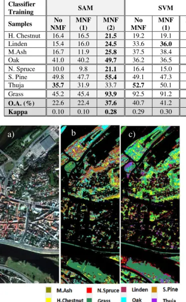
To make sure the classifiers do not favor a class among another, we fixed number of training samples to 100. Also, goal was to test the classifier in rude conditions, with highly heterogeneous distribution of vegetation species over the test zone (Figure 2.a), presence of shadowed areas, and limited ground truth samples for some species of interest. In the literature, the recommended ratio of training data is generally between 50% and 70% (e.g. [14],[15]), for our case study the training sample percentage varied from 2% to 35% of the total set for the 16 bands image, and from 2% to 20% of the total set for the 64 bands image.
SAM classifier was trained with mean training spectra (i.e. the mean is calculated for each training class), so the spectral angle 𝛼 is calculated between the mean references (i.e. training spectral samples) and the target pixels. The classification accuracy over the 16 bands image without MNF is poor; the application of MNF with restoration to the initial space (i.e. MNF-1) doesn’t bring improvements, the classification over the transformed space (MNF-2), improved the accuracy of about 15%, with a global accuracy of 37.6% (Table 2). The SVM classifier seems more robust whatever the image used (i.e. original or using MNF) with increased accuracies (up to 43.6%) (Figure 2.b). Increasing the number of bands from 16 to 64 doesn’t brings improvement using SAM classifier, on the other hand, a
slight increase (2% to 5 %) was noticeable using the SVM classifier whatever the image used with a best accuracy of up to 46.1%, the best visual/statistical accuracy compromise was given by MNF-1 (Figure 2.c.). For the 16 bands image we kept 10 MNF bands depending on their eigenvalues and the improvement compared to the original space was relatively important. For the 64 bands image, 35 MNF bands were kept depending on their eigenvalues. Given the SVM results over the 64 bands MNF images (Table 2), it is likely that an information loss happened, and that we have underestimated the features.
For the 16 bands image, the best detected species (>~50%) are Oak, Pine, Thuja and Grass. For the 64 bands image, the best detected species are Mountain Ash, Oak, Fir, and Grass. The transition from 16 bands to 64 bands is globally better with an enhancement in terms of deciduous species detection, and grass detection, the report concerning the coniferous case is mixed, accuracy for Fir increased, accuracy for Pine and Thuja decreased.
The removal of MNF noisy bands (i.e. feature selection) is a delicate operation (i.e. risk of information loss); many methods are reported in the literature including a selection based on 90% threshold of cumulative MNF variance, or non-unit eigenvalues selection. In addition to the eigenvalues statistical information, other strategies based on visual inspection or entropy measure could be cited (e.g. [8], [16]).
Table 2. Classification accuracies using SAM and SVM classifiers over 16 and 64 bands images.
Figure 2. Vegetation mapping by SVM classifier, a)
original test zone (RGB), b) SVM over 16 bands image and MNF (2), c) SVM over 64 bands image and MNF (1)
5. CONCLUSION
This study presents a performance analysis on vegetation mapping by superspectral/hyperspectral imagery (i.e. 0.5 GSD) using Vis-NIR spectral interval. Eight species were considered in the study with unbalanced ground truth samples, the training samples were fixed to a relatively low value for all the classes, however not favoring any of them in the classification process. We do not manage to find that a distance-based classifier as SAM, is suitable for vegetation mapping, even if a MNF is applied over the original data. The SVM classifier seems more robust over the two datasets
of 16 and 64 bands with overall accuracies between 40% and 46%. The increase of spectral bands enable to enhance the global accuracies of up to 5%, no improvements is noticed for the SAM classifier.
The application of MNF showed an evident enhancement in terms of accuracy especially when classifying over the transformed space, this is supported by the literature in the domain of vegetation mapping (e.g. [17], [14], [18]). Despite the benefit of MNF in terms of data decorrelation and noise removal, the MNF bands selection must be carried using statistical approach by eigenvalues analysis and visual inspection. An under selection of MNF bands could lead to information loss and misclassifications, especially in the transformed domain. Indeed, some of the omitted bands with relatively small eigenvalues caused an over-classification of certain classes (e.g. Grass), meanwhile, many classes were under-classified, especially coniferous and some deciduous trees that were relatively well detected using the 16 bands image (i.e. Table 2, 64 bands SVM with NMF-2).
In terms of land use mapping, the final accuracy performance will generally depend on: (a) study zone context (i.e. highly heterogeneous distribution of species or not). (b) data type (i.e. spatial resolution, spectral resolution, integration of non-optical sensors). (c) Pre-treatments of original data (e.g. bands selection, features selection, filtering). (d) Mapping methods (e.g. pixel-based, object-based, or both), and finally (e) ground truth data used for validation and training steps. In [14] the mapping performance reached accuracies between 65% and 86% over 3 central European test zones using 3 and 5m hyperspectral imagery (i.e. 5 to 7 vegetation species per test zone). In [17] the vegetation mapping accuracy of 7 forest vegetation species was increased when adding a Lidar data to the initial 1m DOQQs aerial imagery from 49% to 71%. In [1] 11 forest vegetation species were mapped using 1m
Veg. species Classif. accuracy (16 bands image) Classif. accuracy (64 bands image) Classifier
Training SAM SVM SAM SVM
Samples No NMF MNF (1) MNF (2) No MNF MNF (1) MNF (2) No NMF MNF (1) MNF (2) No MNF MNF (1) MNF (2) H. Chestnut 16.4 16.5 21.5 19.2 19.1 23.3 11.5 12.1 27.0 28.1 28.0 22.0 Linden 15.4 16.0 24.5 33.6 36.0 35.8 20.5 21.1 13.1 19.3 19.2 17.3 M.Ash 16.7 11.9 25.8 37.5 38.4 46.2 46.3 49.0 50.1 38.5 38.8 34.0 Oak 41.0 40.2 49.7 36.2 36.5 45.8 62.3 61.1 72.9 69.9 72.5 62.2 N. Spruce 10.0 9.8 21.1 16.4 15.0 19.2 26.8 26.9 16.0 50.7 51.6 40.3 S. Pine 49.8 47.7 55.4 49.1 47.3 59.3 10.7 10.5 18.7 17.9 18.1 17.7 Thuja 35.7 31.9 33.7 52.7 50.1 48.3 10.4 10.9 6.7 28.5 27.6 26.8 Grass 45.2 45.4 93.9 92.5 91.2 92.6 22.3 21.8 65.0 85.1 85.5 95.8 O.A. (%) 22.6 22.4 37.6 40.7 41.2 43.6 21.9 22.6 34.5 45.5 45.7 46.1 Kappa 0.10 0.10 0.28 0.29 0.30 0.33 0.11 0.11 0.24 0.34 0.34 0.34
a)
b
)
c)
Panchromatic/4m multispectral IKONOS data, with accuracies of 79% and 86% when filtering the image. In [19] 5 wetland vegetation species were mapped using a 4m CASI-2 imager and pixel/objet-based strategies, the accuracies varied from 56% to 76%. In [8] an accuracy of over 90% was reached for mapping 8 vegetation species using object based approach and Lidar.
This study presents a performance analysis on vegetation mapping by high-resolution superspectral/hyperspectral imagery. The mapping was experimented in a high heterogeneous context in terms of species distribution, and with limited ground truth samples for some species. The used classifiers were trained with moderate and fixed training samples, and a feature selection based on MNF was used. In terms of statistical analysis, the accuracies were not as high in comparison of some above reported studies with quite different and more advantageous data and methods. Nevertheless, the expert validation of the map was encouraging, and the results could be enhanced further using more sophisticated training strategy, and improved feature selection procedure. We showed that a pixel-based strategy preceded by a feature selection step could be an encouraging tool for generating fast and enough reliable vegetation maps in complex context and with limited ground truth data.
6. AKNOWLEDGMENTS
This research was supported by the French National Research Agency (ANR) through the HYEP project (ANR-14-CE22- 0016).
7. REFERENCES
[1] Carleer, A., and E. Wolff, Exploitation of very high resolution satellite data for tree species identification, Photogrammetric Engineering & Remote Sensing, 70(1):135–140, 2004.
[2] Cho, M.A., Debba, P.,Mathieu, R., Naidoo, L., van Aardt, J., and Asner, G.P., Improving discrimination of savanna tree species through a multiple-endmember spectral angle mapper approach: canopy-level analysis, IEEE Trans. Geosci. Remote Sens. 48 (11), 4133–4142, 2010.
[3] Raczko, E., and Zagajewski, B., Comparison of support vector machine, random forest and neural network classifiers for tree species classification on airborne hyperspectral APEX images, European Journal of Remote Sens. 50:1, pages 144-154, 2017. [4] Moskal, L.M., Styers, D.M., and Halabisky, M., Monitoring urban tree cover using object-based image analysis and public domain remotely sensed data, Remote Sens. 3(10): 2243-2262, 2011.
[5] Immitzer, M., Atzberger, C., and Koukal, T., Tree species classification with randomForest using very high spatial resolution 8-Band WorldView-2 satellite data, Remote Sens. 4 (9), 2661– 2693, 2012.
[6] Mozgeris, G., Gadal, S., Jonikavičius, D., Straigyte, L., Ouerghemmi, W. et al, Hyperspectral and color-infrared imaging
from ultra-light aircraft: Potential to recognize tree species in urban environments, 8th Workshop in Hyperspectral Image and Signal Processing: Evolution in Remote Sensing, Aug 2016, Los Angeles, United States. pp.542-546, 2016.
[7] Aksoy S., Gökhan A., and Wassenaar T., Automatic mapping of linear woody vegetation features in agricultural landscapes using very high resolution imagery, IEEE Transactions on Geoscience and Remote Sensing, 48 (1) : 511-522, 2010.
[8] Ballanti, L., L. Blesius, E. Hines, and B. Kruse, Tree Species Classification Using Hyperspectral Imagery: A Comparison of Two Classifiers, Remote Sensing, Vol.8, No. 6, 445, 2016. [9] GOUGEON, F.A. and LECKIE, D.G., The individual tree crown approach applied to IKONOS images of a coniferous plantation area, Photogrammetric Engineering and Remote Sensing, 72, pp. 1287–1297, 2006.
[10] Matthew, M. W., S. M. Adler-Golden, A. Berk, S. C. Richtsmeier, et al., Status of Atmospheric Correction Using a MODTRAN4-based Algorithm. SPIE Proceedings, Algorithms for Multispectral, Hyperspectral, and Ultraspectral Imagery VI. Vol. 4049, pp. 199-207, 2000.
[11] Green, A.A, Berman, M., Switzer, P., and Craig, M.D., A transformation for ordering multispectral data in terms of image quality with implications for noise removal, IEEE Transactions on Geoscience and Remote Sensing 26:65–74, 1988.
[12] Vapnik, V.N., The Nature of Statistical Learning Theory, New York: Springer-Verlag, 1995.
[13] Kruse, F. A., A. B. Lefkoff, J. B. Boardman, K. B. Heidebrecht, A. T. Shapiro, P. J. Barloon, and A. F. H. Goetz, “The Spectral Image Processing System (SIPS) – Interactive Visualization and Analysis of Imaging spectrometer Data.” Remote Sensing of Environment, v. 44, p. 145 – 163, 1993. [14] Fassnacht, F.E., Neumann, C., Förster, M., Buddenbaum, H., Ghosh, A., Clasen, A., Joshi, P.K., Koch, B., Comparison of feature reduction algorithms for classifying tree species with hyperspectral data on three central European test sites. IEEE J. Sel. Top, in Appl. Earth Obs. Remote Sens. 7 (6), 2547–2561, 2014.
[15] Zhang, C., Z. Xie, and D. Selch, Fusing LiDAR and digital aerial photography for object-based forest mapping in the Florida Everglades, GIScience & Remote Sensing, 50:562– 573, 2013. [16] Edurne, I.U. et al. “Assessment of Component Selection Strategies in Hyperspectral Imagery.” Entropy 19 (2017): 666. [17] Zhang, C. and Xie, Z. Object-based vegetation mapping in the Kissimmee River watershed using HyMap data and machine learning techniques. Wetlands, 1–12, 2013.
[18] Ghosh, A., Fassnacht, F.E., Joshi, P.K., Koch, B., A framework for mapping tree species combining hyperspectral and LiDAR data: Role of selected classifiers and sensor across three spatial scales, Int. J. Appl. Earth Obs. Geoinf. 26, 49–63, 2014.
[19] Kamal, M., Phinn, S., Hyperspectral Data for Mangrove
Species Mapping: A Comparison of Pixel-Based and Object-Based Approach. Remote Sens. 3, 2222-2242, 2011.