HAL Id: hal-02556267
https://hal.archives-ouvertes.fr/hal-02556267
Submitted on 27 Apr 2020HAL is a multi-disciplinary open access
archive for the deposit and dissemination of sci-entific research documents, whether they are pub-lished or not. The documents may come from teaching and research institutions in France or abroad, or from public or private research centers.
L’archive ouverte pluridisciplinaire HAL, est destinée au dépôt et à la diffusion de documents scientifiques de niveau recherche, publiés ou non, émanant des établissements d’enseignement et de recherche français ou étrangers, des laboratoires publics ou privés.
Optimisation of the aggregation and execution rates for
intersecting operation sets: an example of machining
process design
Alexandre Dolgui, Genrikh Levin, Boris Rozin
To cite this version:
Alexandre Dolgui, Genrikh Levin, Boris Rozin. Optimisation of the aggregation and execution rates for intersecting operation sets: an example of machining process design. International Journal of Production Research, Taylor & Francis, 2020, 58 (9), pp.2658-2676. �10.1080/00207543.2019.1629668�. �hal-02556267�
Preprint
[article published in International Journal of Production Research]
Alexandre Dolgui, Genrikh Levin & Boris Rozin (2020) Optimisation of the aggregation and execution rates for intersecting operation sets: an example of machining process design,
International Journal of Production Research, 58:9, 2658-2676,
DOI:10.1080/00207543.2019.1629668
OPTIMIZATION OF THE AGGREGATION AND EXECUTION RATES FOR
INTERSECTING OPERATION SETS: AN EXEMPLE OF MACHINING
PROCESS DESIGN
Alexandre Dolgui*, Genrikh Levin** and Boris Rozin**
* IMT Atlantique, CNRS-LS2N, B.P. 20722 F-44307 NANTES Cedex 3, France (e-mail: [email protected])
** United Institute of Informatics Problems, National Academy of Sciences of Belarus Surganov Str, 6, 220012, Minsk, Belarus
(e-mail: {levin,rozin}@newman.bas-net.by)
A sequence of multiple parts is processed on a multi-position transfer line of conveyor type. This sequence consists of identical subsequences (batches). The sets of operations executed for each part at each position are given and these sets for different parts can intersect. Some operations executed at one position can be aggregated into blocks of operations. Each block is executed at a uniform rate (in particular, feed per minute) by a common drive unit. The set of potentially feasible blocks is specified. We consider the situation when the sets of operations for different blocks do not intersect and each potential block can be executed either completely aggregated (i.e. as one block) or completely disaggregated (individually). Aggregation reduces the investment costs, but can increase the consumption of tools due to excluding the individual selection of rates for aggregated operations. The accepted option of the aggregation and the rates of operations remain invariable during the line functioning. The problem is to select the optimal option of aggregation and rates of all operations that minimize the total batch processing cost while ensuring the required line productivity. A mathematical model of the problem and a two-level decomposition method for its solution are proposed. The statement of the problem and the results of its solution are illustrated on a real industrial example. The developed model and method can be applied to solve similar problems arising in other domains.
Keywords: Transfer lines, Batch processing, Aggregation of operations, Operation rate, Operation costs and times, Optimization.
1. Introduction
In last decades, significant attention was paid to the process planning for complexes of interrelated operations in various engineering, organizational and production systems (see, for example, Szadkowski 1971; Alting and Zhang 1989; Boysen, Fliedner and Scholl 2007; Bukchin and Rubinovitz 2003; Halevi 2003; Battaïa and Dolgui 2013). The development of models and methods for joint optimization of the structure of these complexes and execution rates of their operations is of considerable scientific and practical interest.
In this paper, one of the possible approaches to solve such problems is developed. It is illustrated with an example of optimization of transfer line structure and parameters for multi-product batch machining. A multi-position single-flow transfer line of conveyor type is considered (see, in particular, Dolgui et al. 2016, Battaïa et al. 2017).
It is assumed that input sequence of parts is composed of identical sub-sequences of parts (batches). A set of all operations which must be executed at the line for each part as well as an assignment of the operations to the line positions (stations) are given. The term "operation" refers to a set of interrelated machining steps (e.g., milling, drilling, reaming etc.) that is considered as an indivisible action executed at one position (station) by a common drive unit.
The working stroke and range of possible values of the feed per minute used to process a specific part by a drive unit dealing with an operation are given for all parts and operations.
For the sake of terminological generality with other possible application areas, the working stroke will be considered as the volume of operation and will be given for each pair “operation-part”. Similarly, the feed per minute employed for an operation will be considered as the operation rate and also defined for each pair “operation-part”. It is assumed that, with a sufficient accuracy for the considered stage of the manufacturing process design, selected operation rates determine all other machining conditions of operations (cutting speeds, feeds per revolution, etc. for all their machining steps) taking into account the corresponding machining technologies (see, for example, Levin and Rozin 2009).
Parts are machined successively one by one at each working position in the order of their arrival and in the order of location of the positions in the transfer line. At each time point only one part is disposed at each position. Sets of operations executed at a position for different parts can intersect.
At the stage of the machining process planning some operations can be aggregated into blocks. All operations of the same block are executed simultaneously by using the same drive unit with a common operation rate (for example, by using a common multi-spindle head). The volume of each block of operations is the maximum of volumes of its operations.
The aggregation of operations into blocks reduces investment and maintenance costs but excludes the possibility of individual selection and optimization of operation rates for aggregated operations. The latter can lead, in particular, to an increase of operation durations, operating costs, the cost and time related to the consumption of tools and their replacement. Feasibility of an aggregation depends on both the mutual disposal of the machined features of the parts and the capabilities of the available equipment.
The paper deals with the case when all operations of the same potential block can be performed either completely aggregated (in the block) or completely disaggregated (individually). It is impossible to execute a part of block in the aggregated manner and the rest individually, otherwise the corresponding part of block is considered as a block.
The selected option of aggregation of operations and their rates largely determine the structure and parameters of the machining process, the layout of the line as well as the characteristics of the line equipment. Therefore, this decision significantly affects the output of the line, the line investment cost, operational cost, tool consumption and, consequently, the total cost of batch machining.
The objective is to select aggregation options and rates for all operations minimizing the total cost of batch machining while providing a required output of the line.
The rest of the paper is organized as follows. A brief review of literature related to the considered problem is reported in Section 2. The problem statement and its mathematical model are presented in Section 3. The solution techniques based on two-level decomposition scheme are described in Section 4. Section 5 is devoted to industrial example illustrating the proposed approach. Finally, Section 6 includes conclusion remarks. The appendix contains a table of notations used in the paper.
2. Breaf review of literature
One of the first papers on optimization of execution of operation sets in machining systems with a graph approach was published by Szadkowski (1971). Several aspects of the structural and parametric optimization of machining processes in a transfer line of conveyor-type composed of aggregate machines were studied by Levin and Tanaev (1978). Comprehensive surveys of machining process planning articles are presented by Alting and Zhang (1989), and Halevi (2003). A number of articles, e.g. (Bennett and Yano 2004), (Singh and Jebaraj 2005), and (Gupta et al. 2011), were devoted to problems of complex process planning including equipment selection. Singh and Jebaraj (2005) used feature-based environment and operation-based feature mapping to design the set of operations for machining a given part. Then they applied genetic algorithm to find an optimal (for the selected objective function) sequence of operations, machines and cutting tools with respect to a given factory environment. Gupta et al. (2011) developed an integrated model to find an optimal sequence of operations for a given set of machines, tools and machining conditions minimizing the cost of machining cylindrical parts. Bennett and Yano (2004) developed models for selection of equipment in multi-product production systems taking into account capacity consumption, product routing, and impact on the environment.
Joint problems of process planning and scheduling were considered by Mohapatra, Benyoucef and Tiwari (2013). In (Koren, Gu and Guo 2018) the impact of configuration of production system for high-volume manufacturing on the enterprise long-term profitability considering investment cost, throughput, responsiveness to market changes and product quality, was analyzed.
A number of process planning studies have been devoted to the problems of machining conditions optimization, e.g. Arezoo, Ridgway and Al-Ahmari (2000), Cakir and Gurarda (2000). Arezoo, Ridgway and Al-Ahmari (2000) addressed the problems of selection of cutting tools and conditions of machining operations using an expert system. Cakir and Gurarda (2000) suggested a procedure to calculate machining conditions of multi-tool multi-pass milling operations to minimize the production cost.
Among other related problems studied in the literature should be mentioned machining and assembly line balancing problems, that consider allocation of operations to working stations, e.g. Boysen, Fliedner and Scholl (2007), Bukchin and Tzur (2000), Bukchin and Rubinovitz (2003), Dolgui, Guschinsky and Levin (2009), Kara et al. (2011), Battaïa and Dolgui (2013), Battaïa et al. (2017).
The problem considered here is novel and more complex. The nearest problems to it with common elements are those of structural parametric optimization of machining processes in a transfer line of conveyor-type composed of machine tools reported by Levin and Tanaev (1978) and the line balancing problems with equipment selection considered in (Bukchin and Tzur 2000; Bukchin and Rubinovitz 2003). Levin and Tanaev (1978) studied the same type (as in this work) of transfer lines, but they considered processing only homogeneous parts. Also, the selection of an optimal aggregation from a set of feasible aggregation options was not considered in that work. Bukchin and Tzur (2000), Bukchin and Rubinovitz (2003) considered only the case where the intensities of operations execution were uniquely determined by the equipment option selected from a finite set, the possibility of the intersection of sets of operations was not studied. In this paper, the problem consists in selection of an optimal option of aggregation and rates of all operations minimizing the total batch processing cost while ensuring the required line productivity.
There are also our recent papers (Levin, Rozin and Dolgui 2012; Levin, Rozin and Dolgui 2014; Dolgui et al. 2016; Levin, Rozin and Dolgui 2016), where some models and methods for solving problems related to the optimization of execution rates of a collection of intersecting operation sets have already been proposed. But, in that studies the selection of the structure of a collection of intersecting operations and of respective pieces of equipment for their execution were not considered. Note that each of the problems considered in (Levin, Rozin and Dolgui 2012; Levin, Rozin and Dolgui 2014; Dolgui et al. 2016; Levin, Rozin and Dolgui 2016) is a special case of the problem studied in this paper.
To summarize, some aspects of the considered problem were already studied in the above mentioned publications, but no one of these articles has addressed the problem as a whole.
3. Statement of the problem and its mathematical model 3.1. Outline of a machining process and a transfer line
A process of machining multiple parts at a multi-position single-flow transfer line with linearly ordered (working) positions is considered. The input sequence of machined parts is composed of cyclically repeated identical subsequences (batches) {1,...,n}, including all parts of a given list M; some parts
dM in the batch can be repeated, i.e. n|M|. Parts are machined successively one by one at each working position in the order of their arrival and location of the positions in the transfer line. At each position for each part a given set of machining operations are executed in parallel (simultaneously). The sets executed at the same position for different parts can intersect. It is assumed that the same operation for different parts is executed by the same tools, but some of its parameters (in particular, the working stroke, cutting lengths, etc.) for different parts can differ.
The process consists of takts of simultaneous machining all parts located at respective positions. At each time point only one part is disposed at each position. After completing the current takt, all processed parts are moved simultaneously to their next respective working position. The part from the terminal position leaves the line and the next one of the input sequence is loaded to the first position. Then the following takt is executed. The subsequence of n takts that result in the production of one batch constitute the cycle of the batch processing. Without loss of generality, we assume that in takt 1 part 1 of subsequence is located at position 1. Then in the takt i=1,…,n in position k=1,2,… the part dik=(i,k) is processed, where (i,k)=1mod((nimod(k,n)),n) is the index of this part in the batch .
Subsequently, J is the given set of all operations executed at all line positions for all parts and Ji is
the subset of the operations from J executed in takt iI={1,...,i,...,n}.
Table 1. Allocation of parts to positions in takts of a machining cycle Positions Takts 1 2 3 4 5 6 1 1/1 6/4 5/3 4/3 3/2 2/1 2 2/1 1/1 6/4 5/3 4/3 3/2 3 3/2 2/1 1/1 6/4 5/3 4/3 4 4/3 3/2 2/1 1/1 6/4 5/3 5 5/3 4/3 3/2 2/1 1/1 6/4 6 6/4 5/3 4/3 3/2 2/1 1/1
Figure 1 illustrates a layout of such a transfer line.
Table 1 presents an allocation of parts of the batch =(1,1,2,3,3,4) to the positions of a 6-position transfer line in different takts of one cycle of machining (index of the part in the sequence /its type). In general, identical operations may be executed at different positions and the set I of takts of the cycle may include identical takts. However, to simplify the presentation, here all takts in a cycle and operations of different positions are considered as different, i.e. each operation jJ is executed at its own position k(j). In this case, the takt iI and the operation jJi determine the part dij machined by this
operation in this takt. This makes it possible to exclude subsequently from consideration the position indices in the variables.
1 loading position Parts 2 n-2 Spindle heads 2 3 4 5 working positions n-1 n-4 n 1 3 n-3
Figure 1. An example of part allocation in the first takt for the first 5 positions
In this paper, the case when the feed per minute of an operation is the same for all parts processed is considered.
The following notations are introduced (see in the Appendix the table with all notations): - Ljd is the given (minimal required) working stroke of the respective drive unit for operation jJ
when machining part dM, Ljd = 0 if operation j is not executed for d;
- Sj= [Sj1, Sj2] is the given range of feed per minute Sj for operation jJ considering that this
operation is executed for different parts (value Sj is to be determined).
At the design stage of a machining process and transfer line, some operations can be aggregated in blocks. All operations of a block are executed in parallel by the same drive unit (in particular with the use of a single multi-spindle head) with common feed per minute and working stroke. We study the case when (i) the possibilities of aggregation of operations jJ into blocks are specified by a family W of non-unit nonintersecting subsets w of operations from J, (ii) each subset wW can be executed either completely aggregated (i.e. as one block) or completely disaggregated (i.e. as |w|
individual operations), (iii) any combination of aggregation/disaggregation option of potential blocks is possible.
Let qw=0 if all operations from w are executed in aggregate manner and qw=1 otherwise. The
requirement of a common feed per minute for all operations of the block excludes the possibility of selecting the best machining conditions for each of its operations individually. It is assumed that for
wW the common working stroke (for qw=0) of all operations jw when machining part d is
Lwd= max{Ljd|jw} and jwSj because otherwise operations from w cannot be executed in one
block. Further, q=(qw| wW) and Q is the set of possible options of vector q to be selected, |Q|2|W|.
The case when the selected aggregation option and the feed per minute for all operations remain invariable during the line functioning is considered.
An example of execution of two operations from a subset wW for part dM is shown in Figure 2a) for their disaggregated execution and in Figure 2b) for their aggregated option. In the first case the working strokes Lj1d, Lj2d and feeds per minute Sj1, Sj2for operations j1 and j2 are
individual. In the second case, these operations have common working stroke Lwd = max{Ljd|jw}= d
j
L1 and a feed per minute SwSj1 Sj2.
a) b)
Figure 2. Disaggregated (a) and aggregated (b) execution of operations j1 and j2 Tools Spindles Part d Part d j1 j2 j1 j2 w={j1, j2}
It is assumed that operations of one position can be aggregated into several blocks and each block can comprise operations executed for different parts processed at respective position in different takts.
As was above mentioned, it is assumed that with an accuracy sufficient for considered stage of the manufacturing process design, the selected feed per minute of each operation allows to determine (for the accepted aggregation option) other components of its machining conditions. In turn, that makes it possible to estimate for each tool its average life time and consumption, for machining a single batch.
Decisions on how operations are aggregated into blocks as well as decisions on feeds per minute for each block are made at the line design stage and remain invariable (at least during a large period of its operating time). Therefore, the choice of the most rational joint decisions regarding these important characteristics of the structure and the parameters of the manufacturing process are crucial.
In the next subsection, the dependences of the components of productivity and the cost of the manufacturing process on the selected decisions are considered.
In the future, for the convenience of presentation of the proposed mathematical model of the considered problem and the methods for solving it, parameter Sj of operation j is substituted for parameter
uj=1/Sj which we will call “operation rate”. It is obvious that ujUj=[uj1,uj2]=[1/Sj2,1/Sj1]. As operation
jJ in takt iI is executed for part dij, value Lij=
ij
jd
L will be considered as the “volume” of this operation
in this takt. Operation rate means the time spent for execution of a unit of volume of this operation. Since all operations j from block wW should have the same operation rate uj then ujUw=
[U1w=max{u1j|jw}, U2w=min{u2j|jw}] . For fixed qQ the sought vector u=(uj|jJ) must be
selected from the set U(q)={uU|uj ujUw for any j, jw and wW if qw=0}, where U=
J
j j
U .
The following additional assumptions are used in this study:
1. Operations performed at different working positions of the line, as well as all takts of the cycle for processing a batch of parts, are considered as different.
2. The sets of operations of potential blocks do not intersect.
3. All operations of each of the potential blocks can be performed either completely aggregated (in the block) or completely disaggregated (individually), no possibility to aggregate only a part of block.
4. All operations aggregated in one block are performed with the same intensity.
It should be noted that the proposed methods do not need assumption 1 and can be applied without it, but the presentation of the mathematical model will be much complicated. The generalization of the rest of these assumptions requires additional research.
3.2. Cost and time of batch machining
In the considered problem statement, the components of the total cost and total time for machining one batch for the fixed values of vectors qQ and uU can be defined as follows.
Let 1(q,u)=11(q,u)+12(q,u) and 2(q,u)=21(q,u)+22(q,u) be the dependences of the total cost and the total time of one cycle of machining the batch on values of vectors q and u (which are decision variables).
The term 11(q,u) takes into account salary, depreciation of equipment, its maintenance cost, overheads, etc. The term 21(q,u) takes into account besides the operating time also the time for tools replacement, maintenance time, etc. In turn, the terms 12(q,u) and 22(q,u) take into account the cost and time related to the consumption of tools per one cycle of machining the batch , respectively. The terms 11(q,u) and 21(q,u) are considered usually as linearly dependent on the net duration of the cycle of machining the batch :
p1(q,u) = 0( ) 1( ) (max{ | } bi) I i ij j i p p G L u j J t G q q , p=1,2. (1)
Here and below the p=1 refers to the cost and p=2 to the time.
In (1), Lijuj is the duration of operation j in takt i; max{Lijuj | jJi}+tbi is the net duration of takt
i; (max{ | } bi)
I
i Lijuj jJi t is the net duration of the cycle, where tbi is the auxiliary time (e.g. the
duration of idle movements); Gp0(q) are components of cost and time related to a single cycle of
machining that do not depend on the cycle net duration.
Components G11(q) and G21(q) are values of respective cost and time per unit of the cycle net duration. Coefficients Gpl(q) depend on the accepted option q of aggregation and are assumed to be
given for all possible q, p=1,2, l=0,1. Coefficients Gp0(q) allow to take into account in particular the
situation when the production line is designed for a fixed output.
In many real-life situations, with a sufficient accuracy, the following form of these functions can be used:
Gpl(q)=Epl+wW(Eplw(1–qw)+eplwqw),
where Epl0 takes into account the piece of the cost (or time) that does not depend on aggregation of
operations, Eplw0 and eplw0 take into account the piece of the cost (or time) related to aggregated or
disaggregated executing the operations of wW, respectively. Further it is assumed that Eplw<eplw for
all p=1,2, l=0,1, and wW.
Let consider in more detail the terms 12(q,u) and 22(q,u). Note, that these terms depend mainly on rates u, but the range U(q) of possible values of vector u is determined by the selected
values for q. In this paper, when selecting uU(q), it is assumed that tools are replaced independently from each other as they wear. Note that an approach to optimize machining conditions under group replacement of tools was considered in (Levin and Rozin 2009).
Let Rj be the set of tools executing operation jJ and Nijr(uj) be the estimated number of parts
dij machined by this tool during its life time Trd (uj)
ij under assumption that tool r machines only the
part dij. The value Nijr(uj)=Trd (uj)/(ljrd uj)
ij
ij , where ljrdijis the given machining length of machining
part dij by tool rRj, and 0
ij
jrd
l , if tool rRj does not machine part dij.
Under individual replacement of worn tools, the average number of cycles of batch machining between replacements of tool rRj is equal to Njr(uj)=
I
i (1/Nijr(uj))
/
1 .
To evaluating the dependence of tool life on the operation rate, we will introduce the following assumptions:
a) The feed per revolution sjr for tool rRj of operation j is the same for all parts dM it
processes. This feed is usually maximized in the possible range (determined by the processing conditions of all the parts), taking into account its possible relations with the feeds of other tools for this operation. Therefore, to simplify it is assumed that the feeds sjr are known in advance for each
tool rRj of each operation jJ. Thus, the selected rate uj of operation j determines the cutting speed
vjrd when processing part d by tool r: vjrd = jrd/uj, where jrd is a given constant depending on the
diameter of machining.
b) As in (Levin and Tanaev, 1978), the dependence of the expected tool life on feed and cutting speed can be presented by the following modification of the well-known Taylor function:
rd rd rd s v C v s Trd rd ,..., 1 min ) ,
( , where ,rd Crd>0, и rd>rd>1 are known constants for the specific processing conditions (material of the part, cutting depth, tool material, etc.), rRj, dM, =1,…,
rd
μ . This modification describes the considered dependence as a concave (in logarithmic scale)
function that is in good agreement with the majority of real life situations for a wide range of feed and cutting speed changes.
In accordance with above mentioned, we obtain the following dependence of the tool life for tool r when processing part dij with operation rate uj (for the simplicity indexes ij for the part dij are
omitted): rdμ rd rdμ j μ μ j rd u C u T min ~ ) ( ,..., 1 , (2)
where rdμ rdμ s C C rdμ rdμ ~ >0.
Hence, cost and time of operation j in takt i (i.e. when machining the part dij) related to the
consumption of tools per one cycle of machining the batch for a fixed ujUj are equal to:
fpij(uj)= r R gpjr/Nijr(uj) j = j max1,..., ( / ) ijrμ rd R r μ μ Cpijrμ uj , p=1,2, iI, jJi, (3) where gpjr is a given cost (p=1) or a given time (p=2) spent on one replacement of tool rRj,
μ rd rd pjr
pijrμ g l ij C ij
C / ~ , ijrμ rdijμ1. It is obvious that functions fpij(uj), p=1,2 are positive
non-increasing convex functions of operation rate ujUj. According to above mentioned, fpij(uj)=0 if
operation j is not executed in takt i.
Thereby for fixed values of vectors qQ and uU(q) the cost 12(q,u) and the time 22(q,u) are defined by the following relations:
iI jJ pij j
p i f u
Φ 2(q,u) ( ), p=1, 2. (4)
Thus, the total cost and total time for machining one batch of parts are defined by the expressions: p(q,u)= 0( ) 1( ) (max{ jd j| i} bi) I i p p G L u j J t G ij q q iI jJi fpij(uj), p=1,2. (5)
3.3. Mathematical model of the problem
The considered problem is to determine an aggregation option qQ for operations from wW and operation rates u=(uj|jJ)U(q) to minimize the total cost 1(q,u) of one cycle of batch machining, provided that the total time 2(q,u) of the cycle (including the time spent on equipment maintenance and worn tools replacement) does not exceed the specified value T0 determined on the basis of the required line throughput. Taking into account the proposed assumptions, this problem is reduced to the following mixed integer nonlinear programming problem:
Minimize
I i j Ji j ij I i bi i j iju j J t f u L G G Φ1(q,u) 10(q) 11(q) (max{ | } ) 1 ( ), (6) s.t. 0 2 21 20 2( , ) G ( ) G ( ) (max{L u|j J } t ) f (u ) T Φ I i j Ji ij j I i ij j i bi q q u q , (7) qQ, (8) uU(q), (9)In the next section, a special method to solve the problem (6) – (9), called further as Problem A, is proposed.
4. Solution technique
The considered approach to solve Problem A is based on the following its properties:
i) the variables of the problem are divided into two heterogeneous groups: |W|-dimensional binary vector q=(qw|wW)Q and |J|-dimensional vector u=(uj|jJ)U with continuous components ujUj;
ii) functions 1(q,u) and 2(q,u) have identical structure;
iii) if q,qQ are such that qq and qwqw for all wW then U(q)U(q) and p(q,u)<
p(q,u) for all uU(q), p=1,2;
iv) under the previous conditions iii), if Gpl(q) = Gpl(q) for all p=1,2, l=0,1, then
p(q,u*(q)) p(q,u*(q)), p=1,2, where u(q) is the solution of Problem A for a fixed q.
4.1. Two-level decomposition scheme
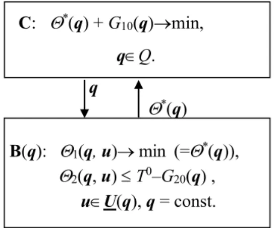
The two-level decomposition scheme proposed to solve Problem A is depicted in Figure 3.
At the lower level, for a fixed vector qQ, the corresponding problem В(q) is solved. A sub-problem В(q) consists in determining the value u(q) of vector uU(q) minimizing the function 1(q,u)=
I ij j i bi i Ij Ji ij j i Lu j J t f u
G11(q) (max{ | } ) 1 ( ) subject to the condition:
2(q,u)= I ij j i bi i Ij Ji ij j i L u j J t f u G21(q) (max{ | } ) 2 ( ) 0 T – G20(q).
At the upper level, sub-problem C to define the vector q* minimizing the function *(q)+G 10(q) is solved, where *(q)=
1(q,u(q)) and *(q)= if sub-problem В(q) is unsolvable.
Figure 3. Decomposition scheme to solve Problem A C: *(q) + G 10(q)min, qQ. q *(q) B(q): 1(q, u) min (=*(q)), 2(q, u) T0–G20(q) , uU(q), q = const.
Since q* and u(q) are solutions of sub-problems С and В(q) respectively, then (q*,u)=(q*,u(q*))
is a solution of Problem A. If q* and u(q*) are approximate solutions of corresponding sub-problems,
then vector (q*, u) is an approximate solution of Problem A.
Below some of possible approaches to solve the obtained sub-problems are presented. For a more detailed consideration of sub-problems В(q) of the lower level, it is necessary to consider if the corresponding operations (and variables associated with them) are executed in the aggregate or disaggregate manner. Since for aggregated execution of some block w, operation rates uj for all
operations jw are the same, then the number of variables of sub-problem В(q) can be reduced. For this, the following additional notations are introduced:
W0(q) = {wW| q
w=0} is a subset of operation blocks from W executed in the aggregate manner
for a fixed qQ;
0
i
W (q) ={wW0(q)|wJi} is a subset of operation blocks from W0(q) that comprise operations executed in takt iI;
J1(q)={jJ|jwW0(q)} is a subset of operations from J that are executed for a fixed q in the disaggregate manner (i.e. with individual rates);
u(q) = (uj|jJ1(q)) and u(q) = (uw|wW0(q)) are vectors of operation rates to be determined for
operations j from J1(q) and for operations j from wW0(q) respectively;
iw = max{Lij|jJiw} is the volume of potential operation block wW executed in iI;
I i pij j j pj u f u f ( ) ( ) ~ and
w j pj w w pw u f ufˆ ( ) ~ ( ) are the functions of cumulative cost (p=1) and
of cumulative time (p=2) for operation jJ and for operation block wW, respectively, on their rates in a single execution of one cycle of batch machining;
p E~ (q)= ( ) 1 \ ( ) 1 1 0 0 q w W W q p w W w p w p E e
E is the cost (p=1) or the time (p=2) of maintenance of
equipment and its depreciation per unit of cycle duration.
Then, for a fixed vector qQ, sub-problem В(q) of the lower level is reduced to the following nonlinear programming problem:
Minimize I i ij j i iw w i bi t W w u Λ J j u L E Θ~( ( ), ( )) ~( ) (max{max{ | 1( )},max{ | 0( )}} ) 1 1 u q u q q q q
) ( 1 ) ( 1 0 1 ) ( ˆ ) ( ~ q q w W w w J j j j u f u f (10) s.t. I i ij j i iw w i bi t W w u Λ J j u L E Θ~ ( ( ), ( )) ~ ( ) (max{max{ | 1( )},max{ | 0( )}} ) 2 2 u q u q q q q0 ) ( 2 ) ( 2 0 1 ( ) ˆ ) ( ~ T u f u f W w w w J j j j q q , (11) ujUj, jJ1(q), (12) uwUw, wW0(q), (13)
where uj, jJ1(q), uw, wW0(q) are decision variables for the fixed vector q.
According to the mentioned above property iii) of Problem A, the vector u*(q) can be used as
an initial point in solving sub-problem В(q) if q q. Possible approaches to solve sub-problem В(q) is largely dependent on the properties of its components. In Dolgui et al. (2016), a special case of Problem A is studied when: (i) volumes Lij for any operation jJ are the same for all iIj, where Ij is
the set of takts from I in which operation j is executed, (ii) values iw for each operation block wW
are identical for all takts iI(w)={iI |wJi}. In this case, the duration of operation jJ as well as
the duration of operation block wW are also the same for all takts iIj and iI(w), respectively. The
proposed approach to this problem is based on a combination of Lagrangian relaxation and Dynamic programming.
Below we will describe the approach to solve В(q) for more frequent case in practice when these volumes can be different.
4.2. Sub-problem В(q)
As above mentioned, in sub-problem В(q) functions ~fpj(uj) and fˆpw(uw) are non-increasing positive and convex on segments Uj and Uw respectively for all jJ, wW. Therefore, the
well-known methods of convex programming are applicable to solve this sub-problem. Furthermore, the last two terms in the functions Θ~1(u(q),u(q)) и Θ~2(u(q),u(q)) are separable. Thus, to solve В(q) it is possible to use, in particular, an approach analogous to the one proposed in (Rozin, Levin, and Dolgui 2013; Levin, Rozin, and Dolgui 2014) which proved to be effective for a similar problem.
This approach is based on approximation of sub-problem В(q) by a linear programming problem.
To describe this approach let us introduce the following piecewise linear approximations of functions~fpj(uj) and fˆpw(uw) on the segments Uj and Uw , respectively:
) ( ~ j pj u f max{apjk uj + bpjk | k=1,…,k1pj}, p=1,2, jJ, (14) ) ( ˆ w pw u f max{cpwk uw + dpwk | k=1,…, k2pw }, p=1,2, wW, (15) where apjk, bpjk, cpwk, dpwk, k1pj and k2pw are parameters of this approximation. Note that these
parameters do not depend on the value of vector q. Thus these approximations can be constructed in advance before the solution of Problem A and can be used to solve problems В(q) for different values of vector q.
Then the approximate solution of problem В(q) for a fixed qQ can be obtained by solving the following linear programming problem:
Minimize
) ( ( ) 1 1 1 1 0 ) ( ~ q q q J j wW w j i I i z y t E , (16) 0 ) ( 2 ( ) 2 2( ) 1 0 ~ T z y t E J j j w W w i I i q q q , (17) ti – Lij uj ≥ 0, iI, jJ1i(q), (18) ti – iwuw ≥ 0, iI, wWi0(q), (19) ypj – apjk uj ≥ bpjk, p=1,2, jJ1(q), k=1,…, k1pj, (20) zpw– cpwk uw ≥ dpwk, p=1,2, wW0(q), k=1,…, k2pw, (21) ujUj, jJ1(q), (22) uwUw, wW0(q). (23)In this problem, vectors t=(ti | iI), y(q) =(ypj| p=1,2, jJ1(q) ), z(q) =(zpw| p=1,2,wW0(q)), u(q) and u(q) are to be defined. If (t,y(q),z*(q),u*(q) ,u*(q)) is its solution then vector u=(uj|jJ) with the components uj=u*j(q) for jJ1(q) and uj=u*w(q) for jwW0(q) can be accepted as an approximate
solution u(q) of problem В(q). The discrepancy between the minimum values of the objective functions of problem В(q) and its approximation (16)-(23) is determined by the accuracy of the approximation (14)–(15) of functions ~fpj(uj) and fˆpw(uw)in the vicinity of solution of problem В(q).
To solve the approximate problem (16)-(23) for fixed values qQ, the existing software tools such as CPLEX or LPSolve can be used. The performance of the proposed approach when solving a sub-problem В(q) using computer Intel Xeon CPU E5320 with parameters 1.86 GHz and 8GB of RAM and the software LPSolve is reported in (Levin, Rozin and Dolgui 2016).
4.2. Sub-problem C
In sub-problem C, the number of possible values of vector q in the set Q may be up to 2|W|, so full enumeration of set Q with solving of sub-problem В(q) for each qQ requires a significant time even for relatively small values of |W| and practically impossible for a large |W|. In such a situation, it seems promising to use methods based on the ideas of random search, heuristics and metaheuristics
in combination with the proposed below a special version of the method of sequential fixing of variables (MSFV).
The algorithm MSFV starts with initial value q0 of vector q obtained using some heuristic approach. This algorithm forms a sequence of vectors from Q, such that each subsequent vector differs from the previous vector by exactly one of its components. The components which values have been changed are considered as fixed and are not altered subsequently. The selection of the next vector of the sequence at the current iteration is performed as follows. For the current vector qc, the
subset Q(qc)Q of vectors that differ from qc by one of its non-fixed components is constructed. For
each vector qQ(qc), sub-problem В(q) is solved. As the next vector of the sequence, the vector qQ(qc) that corresponds to the minimal value of the function H(q)=*(q) +G
10(q) in these sub-problems is selected. The component by which vectors q and qc differ is considered as fixed. The
number of vectors in subsets Q(qc) from iteration to iteration decreases from |W| to 1. Accordingly,
the number of sub-problems В(q) to be solved is also reduced. At each iteration we get (in general) a new improved vector qQ. The algorithm terminates when either the value of H(qc) is not decreased,
or the subset Q(qc)=. The obtained value of qc is taken as the solution of problem C. The total
number of sub-problems В(q) to be solved for calculation of function H(q) for different q does not exceed 0.5(|W|2+|W|).
Below the scheme of the algorithm MSFV is presented, where:
- is a set of wW with fixed values of component qw for current vector qc;
- q(q,w) is a vector from Q that differs from vector qQ only by the component qw.
Algorithm MSFV:
Step 0. Assign qc q0, Yc H(q0), .
Step 1. If =W then qc is a new solution of problem С. Else
Step 2. Find w*=argmin{H(q(q,w))|wW\}. If YcY*= H(q(q,w*)) then assign =W and go to Step 1. Else assign qc=q(q,w*), Yc=Y*, ={w*} and Step 2 is repeated.
The algorithm MSFV can be repeated with a new initial value q0. As such a value, in particular, the current solution obtained earlier can be used. The described algorithm MSFV can be evolved by means of selection at each iteration simultaneously several perspective components of current vector q for their fixing accordingly to the values of function H(q) obtained.
5. Industrial example 5.1. Input data
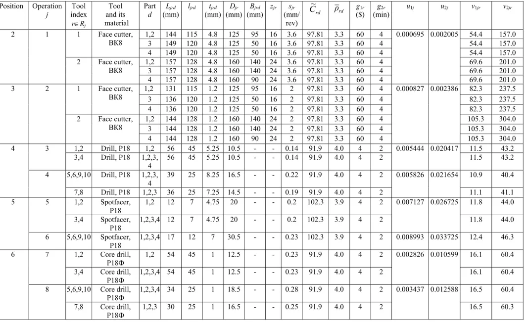
As an illustrative example, we present here a fragment of machining process for a family M={1,2,3,4} of parts processed at a 6-position rotary transfer machine which is a part of a transfer line. This fragment considers the features (faces and holes) of parts from M located at one side of each of these items. The family M of parts and their features to be machined at this machine are depicted in Figure 4. The dimensions of these features are given in Table 2. The material of all parts is gray cast iron with HB=190.
The parts are machined one by one by sequentially repeated identical subsequences (batches). A batch =(1,1,2,3,3,4) is composed of 6 parts: two items of part 1, one item of part 2, two items of part 3 and one item of part 4. The machining the considered features of the parts includes: rough and finish milling for faces 1 and 2, drilling and core drilling for holes 3-7, and spotfacing for all holes with the exception of holes 6.
a) Part 1 b) Part 2
c) Part 3 d) Part 4
Figure 4. The family of parts to be machined
The first position of the rotary machine is used only for loading and unloading of machined parts, others are working positions. Rough and finish milling are executed in the second and third position respectively by the face cutters mounted on a vertical milling head. In positions 4 to 6, the drilling, spotfacing and core drilling are executed by the respective horizontal spindle heads. In the considered
6 4 Face 2 7 6 5 4 3 Face 2 Face 1 7 4 3 Face 1 Face 2 5 Face 1 5 6 7 4 5 7 Face 1 Face 2
case the cycle of machining one batch consists of 6 takts and therefore the fixture of each part can be assigned to its own position of the rotary table. The allocation of parts to working positions in each takt of the cycle is presented in Table 1. The time tbi of table movements (idle time) in each takt is equal to
0.2 min.
The parts are installed on the positions so that the maximum number of machining steps for different parts could be carried out by the same tool. Machining steps are combined in operations (in terms of Section 3) so that each operation is executed by one spindle head. Since the material of all parts is the same we accept that the feed per revolution sjr, the range [v1jr,v2jr] of possible values of
cutting speed vjr as well as parameters of life time in the relation (2) for each tool r are the same for
all machined parts. For simplicity, we assume that μrd 1 for all tools and all parts. Feed per revolution sjr and range [v1jr,v2jr] determine the ranges Uj=[u1j, u2j] of possible values of rates uj of
operations. Thus, in the relations (3) values ijr are the same for all rRj and equal to ij:
ij j pij j pij u C u f ( ) , (24) where j R r pijr pij C С .
Input data for machining process design are given in Table 2. These data include: operations executed at each position for each part; tools and their parameters; parameters of relation (2) for respective machining steps; cost and time spent for replacement of each tool. In Table 2, the following notation are used:
- Ljrd, ljrd, tjrd, Bjrd are the working stroke, the cutting length, the depth of cut and the machining
width for tool r in operation j when machining part d, respectively;
- Djr , zjr and sjr are the diameter, the number of teeth (for cutter) and the feed per revolution of
tool r in operation j, respectively;
- u1j, u2j are the lower and upper bounds of the range for the rate of operation j;
- v1jr, v2jr are the lower and upper bounds of the range of cutting speed for tool r in operation j; - C~rd, ρ are the parameters in the relation (2) for tool r when machining part d; rd
Table 2. Parameters of part features, tools, machining steps, tool life relations and structure of operations. Position Operation j index Tool rRj Tool and its material Part d (mm)Ljrd ljrd tjrd (mm) (mm)Djr (mm)Bjrd zjr (mm/sjr rev) rd C~ ρrd ($) g1r (min)g2r u1j u2j v1jr v2jr 2 1 1 Face cutter, ВК8 1,2 3 144 115 149 120 4.8 4.8 125 125 95 50 16 3.6 16 3.6 97.81 97.81 3.3 3.3 60 60 4 4 0.000695 0.002005 54.4 54.4 157.0 157.0 4 149 120 4.8 125 50 16 3.6 97.81 3.3 60 4 54.4 157.0 2 Face cutter, ВК8 1,2 3 157 128 157 128 4.8 4.8 160 140 24 3.6 160 140 24 3.6 97.81 97.81 3.3 3.3 60 60 4 4 69.6 69.6 201.0 201.0 4 157 128 4.8 160 90 24 3.6 97.81 3.3 60 4 69.6 201.0 3 2 1 Face cutter, ВК8 1,2 3 131 115 136 120 1.2 1.2 125 125 95 50 16 16 2 2 97.81 97.81 3.3 3.3 60 60 4 4 0.000827 0.002386 82.3 82.3 237.5 237.5 4 136 120 1.2 125 50 16 2 97.81 3.3 60 4 82.3 237.5 2 Face cutter, ВК8 1,2 3 144 128 144 128 1.2 1.2 160 140 24 160 140 24 2 2 97.81 97.81 3.3 3.3 60 60 4 4 105.3 105.3 304.0 304.0 4 144 128 1.2 160 90 24 2 97.81 3.3 60 4 105.3 304.0 4 3 1,2 Drill, P18 1,2 56 45 5.25 10.5 - - 0.14 91.9 4.0 4 2 0.005444 0.020417 11.5 43.2 3,4 Drill, P18 1,2,3, 4 56 45 5.25 10.5 - - 0.14 91.9 4.0 4 2 11.5 43.2 4 5,6,9,10 Drill, P18 1,2,3, 4 39 25 8.25 16.5 - - 0.22 91.9 4.0 4 2 0.005826 0.021654 10.9 40.4 7,8 Drill, P18 1,2,3 36 25 7.25 14.5 - - 0.19 91.9 4.0 4 2 11.1 41.1 5 5 1,2 Spotfacer, P18 1,2 12 7 4.75 20 - - 0.2 102.3 3.9 4 2 0.007127 0.026725 11.8 44.0 3,4 Spotfacer, P18 1,2,3,4 12 7 4.75 20 - - 0.2 102.3 3.9 4 2 11.8 44.0 6 5,6,9,10 Spotfacer, P18 1,2,3,4 17 12 7 30.5 - - 0.23 102.3 3.9 4 2 0.008993 0.033725 12.4 46.3 6 7 1,2 Core drill, Р18Ф 1,2 54 45 1 12.5 - - 0.23 91.9 4.0 4 2 0.002826 0.010599 16.1 60.4 3,4 Core drill, Р18Ф 1,2,3,4 54 45 1 12.5 - - 0.23 91.9 4.0 4 2 16.1 60.4 8 5,6,9,10 Core drill, Р18Ф 1,2,3,4 34 25 1 18.5 - - 0.28 91.9 4.0 4 2 0.003437 0.012588 16.5 60.4 7,8 Core drill, Р18Ф 1,2,3 30 25 1 16.5 - - 0.25 91.9 4.0 4 2 16.5 60.3
So in each of positions 4, 5 and 6 two operations (i.e. pairs of operations {3,4}, {5,6} and {7,8} respectively) are executed. Each such a pair of operations can be aggregated into the respective operation block. Thus (see Section 3), the operation set is J={1,2,…,8}, and the family of potential operation blocks is W={w1={3,4}, w2={5,6}, w3={7,8}}, hence possible options of aggregation of operations are presented by the vector q =(q1, q2, q3)Q and |Q|=8.
Each operation block wW is to be executed by one multi-spindle head with common driver, while the disaggregated execution of the respective operations should be performed by two individual spindle heads with their own drivers.
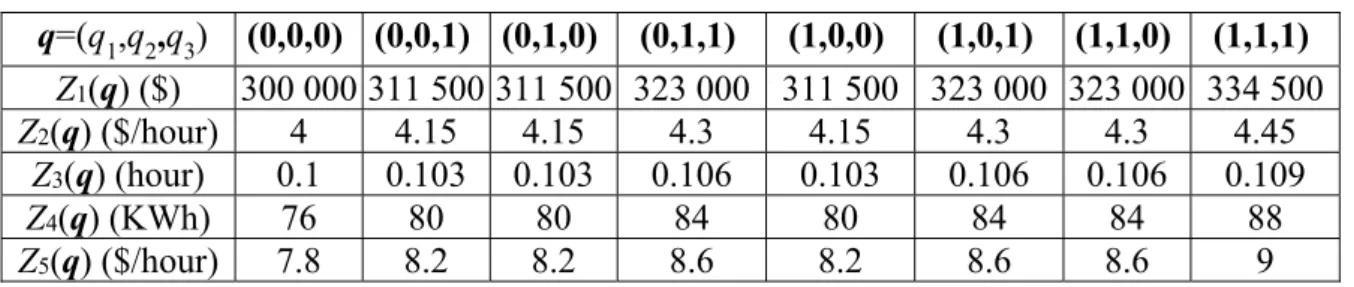
The parameters Gpl(q) in the relations (1) for the four different options O1, O2, O3, O4 of annual (batch production) plan and for all feasible qQ are given in Table 3. In this table T0 is a maximal feasible value of cycle duration for the respective annual plan. It is assumed that values of parameters G11(q) and G21(q) do not depend on annual plan.
Table 3. Parameters Gpl(q) of functions 11(q,u) and 21(q,u)
Ok/T0 q (0,0,0) (0,0,1) (0,1,0) (0,1,1) (1,0,0) (1,0,1) (1,1,0) (1,1,1) 10000/ 20.33 G10(q) ($) G20(q) (min) 36400/ 5.58 G 10(q) ($) 1.36 1.4 1.4 1.452 1.4 1.452 1.452 1.497 G20(q) (min) 0.26 0.273 0.273 0.28 0.273 0.28 0.28 0.289 38900/ 5.22 G 10(q) ($) 1.274 1.316 1.316 1.358 1.316 1.358 1.358 1.4 G20(q) (min) 0.25 0.263 0.263 0.27 0.263 0.27 0.27 0.278 39500/ 5.15 G 10(q) ($) 1.255 1.296 1.296 1.3378 1.296 1.3378 1.3378 1.3794 G20(q) (min) 0.24 0.252 0.252 0.259 0.252 0.259 0.259 0.266 Ok, k=1,2,3,4 G11(q)($/min) 0.7 0.711 0.711 0.722 0.711 0.722 0.722 0.733 G21(q) 1.1 1.103 1.103 1.106 1.103 1.106 1.106 1.109
Table 3 was obtained under the following assumptions. The service life of the transfer machine is 7 years. The number of machine operators is 1 and his labour rate is 7 $/hour. The number of working hours per year is 3987 for 2 shifts per working day. The availability coefficient of the transfer machine is 0.85. The overhead rate is 3.3 (taking into account other staff, general running costs and others items). The average utilization rate of the total engine power of the transfer machine is equal to 0.75. Investment costs Z1(q) of the rotary machine for different aggregation options qQ, the cost Z2(q) and time Z3(q) for maintenance of the rotary machine per unit of operating time, the total engine power Z4(q) of the rotary machineand the energy cost Z5(q) per unit of operating time are given in Table 4. Annual cost of depreciation of the production area and other similar items is equal to 6 700 $ for all aggregation options of the rotary machine.
Table 4 Initial data for determining parameters Gpl(q) q=(q1,q2,q3) (0,0,0) (0,0,1) (0,1,0) (0,1,1) (1,0,0) (1,0,1) (1,1,0) (1,1,1) Z1(q) ($) 300 000 311 500 311 500 323 000 311 500 323 000 323 000 334 500 Z2(q) ($/hour) 4 4.15 4.15 4.3 4.15 4.3 4.3 4.45 Z3(q) (hour) 0.1 0.103 0.103 0.106 0.103 0.106 0.106 0.109 Z4(q) (KWh) 76 80 80 84 80 84 84 88 Z5(q) ($/hour) 7.8 8.2 8.2 8.6 8.2 8.6 8.6 9
Parameters С in the relations (24) for p =1,2, ipij I, jJi are given in Table 5.
Table 5. Parameters С1 and ij С2 (coefficient 10ij –10 common for all values is omitted)
i 1 2 j 1 2 3 4 5 6 7 8 1 2 3 4 5 6 7 8 ij С1 82.7 129.9 3.62 5.049.2127.6 1.3 1.57116.5 100.8 3.62 5.04 4.61 27.6 1.3 1.57 ij С2 5.51 8.66 1.81 2.52 4.6 13.8 0.65 0.79 7.77 6.72 1.81 2.52 2.3 13.8 0.65 0.79 i 3 4 j 1 2 3 4 5 6 7 8 1 2 3 4 5 6 7 8 ij С1 116.5 141.9 3.62 3.4 4.6127.6 0.65 1.57116.5 141.9 7.24 5.04 4.61 27.6 0.65 1.57 ij С2 7.77 9.46 1.81 1.7 2.3 13.80.3240.79 7.77 9.46 3.62 2.52 2.3 13.8 0.3240.79 i 5 6 j 1 2 3 4 5 6 7 8 1 2 3 4 5 6 7 8 ij С1 97.0 141.9 7.24 5.049.2127.6 0.65 1.08 97.0 129.9 7.24 5.04 9.21 27.6 1.3 1.57 ij С2 6.47 9.46 3.62 2.524.6113.80.3240.79 6.47 9.46 3.62 2.52 4.61 13.8 0.65 0.79
5.2. Optimization results and discussion
In Table 6, the results of sub-problem B(q) solution for different options of qQ and plans O1,O2, O3 and O4 are presented. As can be seen, the optimal value of the objective function Ф1(q,u) for the plan O1 is achieved for theaggregation option q=(0,0,0); for the plans
O2, O3 and O4 the optimal aggregation option is q=(1,0,0). For the plan O4, the gain when selecting the aggregation option q=(1,0,0) is more than 6.8% compared to q=(0,0,0).
The optimal values *(q*) j
u and *(q*) j
S of operation rates uj and feeds per minute Sj=1/uj,
jJ, for the optimal aggregation options q*(O
k) for different plans Ok are presented in Table 7.
The optimal values * (q*, *(q*)) j jr u
v of cutting speed vjr for all tools rRj for the optimal values q*(Ok) and operation rates *
j
Table 6. The results for different annual output and aggregation options q (0,0,0) (0,0,1) (0,1,0) (0,1,1) (1,0,0) (1,0,1) (1,1,0) (1,1,1) O1 Ф1(q,u*(q)) 9.2874 9.486 9.4923 9.69 9.3191 9.51 9.524 9.715 Ф2(q,u*(q)) 20.33 20.376 20.376 20.414 20.376 20.414 20.414 20.444 O2 Ф1(q,u*(q)) 5.6917 5.766 5.7723 5.8587 5.5991 5.6772 5.692 5.7635 Ф2(q,u*(q)) 5.58 5.5966 5.5966 5.607 5.5966 5.607 5.607 5.612 O3 Ф1(q,u*(q)) 5.736 5.784 5.834 5.879 5.5181 5.5836 5.6025 5.6675 Ф2(q,u*(q)) 5.22 5.2366 5.2366 5.2472 5.2366 5.2472 5.2472 5.2588 O4 Ф1(q,u*(q)) 5.8862 5.8804 6.0202 5.9893 5.5096 5.57 5.5958 5.6552 Ф2(q,u*(q)) 5.15 5.1656 5.1656 5.1762 5.1656 5.1762 5.1762 5.1868 Table 7. The optimal values *(q*)
j
u and *(q*) j
S of operation rates uj and feeds per minute Sj
Output j 1 2 3 4 5 6 7 8 O1, q*(O 1) * j u 0.0020051 0.0023865 0.0095468 0.0095468 0.0267252 0.026725 2 0.0099004 0.0099004 * j S 498.7231 419.0264 104.7468 104.7468 37.4178 37.4178 101.0058 101.0058 O2, q*(O2) * j u 0.0020051 0.0023865 0.0089628 0.0128697 0.0267252 0.026725 2 0.0092948 0.0092948 * j S 498.7231 419.0264 111.5719 77.7019 37.4178 37.4178 107.5872 107.5872 O3, q*(O3) * j u 0.0020051 0.0023865 0.0086972 0.0124882 0.0267252 0.026725 2 0.0090193 0.0090193 * j S 498.7231 419.0264 114.9802 80.0755 37.4178 37.4178 110.8737 110.8737 O4, q*(O4) * j u 0.0020051 0.0023865 0.0084355 0.0121125 0.0267252 0.026725 2 0.0087479 0.0087479 * j S 498.7231 419.0264 118.5468 82.5594 37.4178 37.4178 114.313 114.313
Table 8. The optimal values * (q*, *(q*))
j jr u v of cutting speed vjr Position 2 3 4 5 6 j 1 2 3 4 5 6 7 8 r 1 2 1 2 1,2,3,4 1,2,5,6 3,4 1,2,3,4 1,2,5,6 1,2,3,4 1,2,5,6 3,4 O1 54.4 69.63 82.28 105.3 24.68 24.68 25.11 11.755 15.588 17.246 20.966 20.94 O2 54.4 69.63 82.28 105.3 26.288 18.308 18.63 11.755 15.588 18.369 22.33 22.31 O3 54.4 69.63 82.28 105.3 27.09 18.867 19.2 11.755 15.588 18.93 23.01 22.99 O4 54.4 69.63 82.28 105.3 27.932 19.453 19.794 11.755 15.588 19.518 23.728 23.702
The models and methods proposed in this work determine optimal design solutions for each specific production system and situation (data).
The results obtained using the proposed models and methods for this use case (and other test cases studied by the authors) lead to the following observations:
1. The optimality of the options for aggregating operations depends on the required annual plan. With its increasing, the positive effect of aggregated execution of some potential operation block is reduced, since the decrease in the unit investment cost is overlapped by the increase in
unit operating costs due to common rate for all operations of this block (i.e. non-optimal operation rates for each operation separately).
2. A given annual plan limits the ability of aggregated execution of some blocks due to narrowing the ranges of the possible common operation rates for the operations of these block. For the considered case study, the maximal productivity 41300 batches/year (i.e. the lowest possible value of the total cycle time T0=4.92 min) is achieved for the completely disaggregated option q=(1,1,1). The maximal productivity for the completely aggregated option q=(0,0,0) is only 39570 batches/year (T0=5.139 min).
3. The effect of aggregation of operations the less, the more the number of different features to be machined by the potential operation block and the greater the difference in parameters (in particular, diameters and lengths) of these features.
4. For an aggregation option that is optimal for some annual plans, a range of annual plans for which this option remains optimal can be defined. In particular, when the plan is less than a certain "boundary" one, the aggregated option for all potential blocks becomes preferable.
These observations are in good agreement with the properties of rational design solutions for this class of production systems.
6. Conclusion
A lot of processes in different application fields (not only manufacturing systems) can be described as sequential execution of a collection of some intersecting operation sets. In this paper, such a class of problems is considered on an example of a problem of structural-parametric optimization of the manufacturing processes of multi-product batch machining on multi-position transfer lines composed of rotary machines is considered. A mathematical model and a method for solving a rather wide class of problems of joint optimization of aggregation of operations of a given collection and the rates of operation execution is proposed. The proposed mathematical model and method can be used for such problems in other applications. The model is formed in terms of mixed integer nonlinear programming and a two-level decomposition scheme to solve it is developed. The upper level sub-problem of the proposed decomposition scheme consists in selecting an aggregation option of operations into blocks. The lower level sub-problem is to determine the execution rates of all operations for fixed aggregation option. The method of approximate solution of the first sub-problem is based on the combination of heuristic methods and a special version of the method of sequential fixing of variables. A widespread in practice special case of the lower level sub-problem is when the cost and the time spent for each of operations are convex functions of their rates. The method
proposed for its solution is based on approximation of this problem by a linear programming problem.
The problem statement and its mathematical model are illustrated with one real life design problem for spindle head aggregation/disaggregation options in machining environment for the design of a rotary machine. The experiments have confirmed very good performance of the proposed methods.
This is a general approach which can be applied to different problems of this type in different real life application domains. Similar problems may arise for example at the design stage for various production systems (in particular, assembly/disassembly lines, lines for testing/repairing complex equipment, etc.) as well as for organizations and service systems.
The promising areas of further research include the following: studying a wider class of problems when:
- a partial aggregation of operations in blocks is allowed (in particular, potential blocks of one position can intersect);
- the opportunities for aggregation and disaggregation of operations at positions are limited by certain additional conditions (in particular, there are restrictions on the number of blocks of operations at some positions);
developing effective methods for exact and approximate solution of the original problem with non-convex functions of cost and time of operations on their execution rates;
developing an iterative scheme for solving the original problem, involving sequential approximation refinement relations according to the previously obtained solutions; developing methods to determine the stability region of solutions;3
show the applicability of the approach in many other real life industrial domains.
Disclosure statement
No potential conflict of interest was reported by the authors.
Acknowledgments
The authors thank E.Tsvirko who performed numerical experiments to verify the proposed methods. This work was partially supported by the region Pays de la Loire (Program “Strategical Recrutment”), France.
References
Alting, L., and H. Zhang. 1989. “Computer Aided Process Planning: the state-of-the-art survey.” International Journal of Production Research, 27(4): 553–585.
Arezoo, B., K. Ridgway, and A.M.A. Al-Ahmari. 2000. “Selection of cutting tools and conditions of machining operations using an expert system.” Computers in Industry, 42: 43–58.