Non-linear unmixing of hyperspectral images using multiple-kernel self-organizing maps

Any correspondence concerning this service should be sent

to the repository administrator:

tech-oatao@listes-diff.inp-toulouse.fr

This is an author’s version published in:

http://oatao.univ-toulouse.fr/24835

To cite this version: Rashwan, Shaheera and Dobigeon, Nicolas

and Sheta, Walaa and Hanan, Hassan Non-linear unmixing of

hyperspectral images using multiple-kernel self-organizing maps.

(2019) IET Image Processing, 13 (12). 2190-2195. ISSN 1751-9659

Official URL

DOI :

https://doi.org/10.1049/iet-ipr.2018.5094

Open Archive Toulouse Archive Ouverte

OATAO is an open access repository that collects the work of Toulouse

researchers and makes it freely available over the web where possible

Non-linear unmixing of hyperspectral images

using multiple-kernel self-organising maps

doi: 10.1049/iet-ipr.2018.5094 www.ietdl.org

Shaheera Rashwan

, Nicolas Dobigeon

_{, Walaa Sheta}

_{, Hanan Hassan}

1_{Informatics Research Institute, City of Scientific Research and Technological Applications, Alexandria, Egypt} 2_{University of Toulouse, IRIT/INP-ENSEEIHT, 31071 Toulouse Cedex 7, France}

E-mail: srashwan@enseeiht.fr

Abstract: The spatial pixel resolution of common multispectral and hyperspectral sensors is generally not sufficient to avoid that

multiple elementary materials contribute to the observed spectrum of a single pixel. To alleviate this limitation, spectral unmixing is a by-pass procedure which consists in decomposing the observed spectra associated with these mixed pixels into a set of component spectra, or endmembers, and a set of corresponding proportions, or abundances, that represent the proportion of each endmember in these pixels. In this study, a spectral unmixing technique is proposed to handle the challenging scenario of non-linear mixtures. This algorithm relies on a dedicated implementation of multiple-kernel learning using self-organising map proposed as a solver for the non-linear unmixing problem. Based on a priori knowledge of the endmember spectra, it aims at estimating their relative abundances without specifying the non-linear model under consideration. It is compared to state-of-the-art algorithms using synthetic yet realistic and real hyperspectral images. Results obtained from experiments conducted on synthetic and real hyperspectral images assess the potential and the effectiveness of this unmixing strategy. Finally, the relevance and potential parallel implementation of the proposed method is demonstrated.

1 Introduction

With the recent and rapid development of hyperspectral imaging technology, hyperspectral images have been widely used in various scientific fields, such as environmental mapping, risk prevention, urban planning, pollution monitoring and mining exploration [1]. Even if classical processing tasks of hyperspectral image analysis include dimensionality reduction, object detection and image segmentation/classification, spectral unmixing certainly remains the most investigated technique to extract relevant information from the observed scene while facing with the generally limited spatial resolution of the sensors. Indeed, the raw spatial resolution of standard hyperspectral sensors usually leads to observing mixed pixels, i.e. which are composed of more than one elementary material. Separating these mixed pixels into a set of elementary material spectral signatures (or endmembers) and estimating their corresponding fractions (or abundances) in each pixel is an automated procedure known as spectral unmixing or spectral

mixture analysis [2].

There are two main classes of mixing models commonly advocated to relate the observed pixel spectrum to the endmember spectra and abundances. The first one, referred to as a linear mixing model (LMM), assumes that the observed spectra result from linear combinations of the endmember signatures. Conversely, a wide class of non-LMMs (NLMMs) covers a large variety of applicative contexts where LMM fails to accurately describe the mixing process underlying the observations. Although LMM is easy to implement and to handle in common scenarios, considering NLMM may be inevitable when analysing more complex scenes, e.g. characterised by multi-layer structures, such as vegetated areas [3] or urban canyons [4], or by intimate sand-like mixtures [5]. The interested reader is invited to consult [6–8] for comprehensive discussions on both classes of models.

Most of the unmixing strategies are based on two-step procedures. Firstly, the spectral signatures associated with the endmembers are extracted from the whole set of image pixels. Secondly, in an inversion step, the abundances are estimated in each pixel based on the estimated endmembers and the adopted LMM or NLMM. Popular endmember extraction algorithm includes N-FINDR [9] and simplex growing algorithm (SGA) [10]

which search for a simplex with the maximum volume inscribed in the dataset. Similarly, pixel purity index (PPI) [11] and vertex component analysis (VCA) [12] recovers this simplex through geometrical projections. Regarding the inversion step, in the past decades, many algorithms based on LMM have been developed to recover the abundances associated with each pixel measurement. Heinz and Chang [13] introduced the popular fully constrained least squares (FCLS) unmixing method based on LMM. It is based on a least-squares approach that simultaneously exploits the so-called abundance of sum-to-one and non-negativity constraints. More recently, Bioucas-Dias and Figueiredo [14] introduced two algorithms, referred to as Sunsal and C-Sunsal, to solve a class of optimisation problems derived from the LMM-based spectral unmixing formulation. The proposed algorithms are based on the alternating direction method of multipliers, which decomposes the initial problem into a sequence of easier ones, with the great advantage of being much more computationally efficient than FCLS.

When dealing with non-linear mixtures, dedicated unmixing techniques should be considered. Some of them proposed in the literature rely on parametric formulations of the non-linearities that may occur during the mixing process. When these non-linearities result from multiple scattering effects, various bilinear mixing models have been designed [15] for which specific unmixing techniques have been developed [4, 16, 17]. Conversely, non-parametric model-based unmixing strategies have been derived to address a larger variety of linear mixtures. When the non-linearities are considered as additional contributions of the LMM, robust models allow these non-linear terms to remain unspecified [18, 19]. Additionally, some significant contributions exploit the versatility of the machine learning framework to handle the variety of non-linear effects, in particular when training dataset are available to learn the non-linear mapping from the abundances to the measured pixel spectra. For instance, a neural network approach has been proposed in [20] to tackle the unmixing problem by two successive stages: the first one reduces the dimension of the input data, and the second stage performs the mapping from the reduced input data to the abundance coefficients. In [21], extreme learning machines are implemented to train a regression model

subsequently resorted to recovering the abundances of target classes.

Besides, multiple-kernel learning (MKL), which is known as learning a kernel machine with a set of basis kernels, has been developed in machine learning area [22] to solve optimisation problems arising when conducting an SVM-classification task. MKL can also be envisaged to address unmixing problems. Such a framework has several advantages: (i) it can simultaneously use numerous features (computed from the different bands of the hyperspectral images) to enrich the data similarity representations, (ii) it is an intermediate combination of data which means that the mixed pixel is preserved during the process without loss of information in its early combinations [22] and (iii) it can be easily parallelised to speed up the computation [23]. To this end, Liu et

al. [24] have proposed a framework called multiple-kernel

learning-based spectral mixture analysis (MKL-SMA) that integrates an MKL method into the training process of linear spectral mixture analysis. They derived a closed-form solution of the kernel combination parameters, unlike most MKL approaches. Similarly, Chen et al. [25] have formulated the problem of abundance estimation resulting from non-linear mixtures based on an MKL paradigm. Also, Gu et al. [26] have shown that integrating reproducing kernel Hilbert spaces (RKHSs) spanned by a series of different basis kernels in multiple-kernel Hilbert space can empower handling general non-linear problems more easily than traditional single-kernel learning. All these methods are based on MKL with an SVM-based solver. Thus, per se, they are supervised learning since they need a priori knowledge on the estimated endmembers and abundances. Unfortunately, in most applicative context, this prior knowledge is not available. To overcome this limitation, this paper suggests replacing the usual solver by the neural network, the Kohonen's self-organising maps (SOMs) [27]. The non-linear unmixing model proposed in this paper boils down to an appropriate implementation of multiple-kernel SOM (MK-SOM) specifically designed to solve the unmixing problem. This simple and intuitive strategy opens promising routes since, in particular, it is highly parallelisable, which can lead to an easy VLSI implementation based on systolic arrays or FPGAs, and it is easily expendable to a high number of dimensions [28].

The paper is organised as follows. Section 2 presents the proposed MK-SOM unmixing strategy, focusing on the training and testing algorithms. Section 3 provides the experimental results we have obtained after applying the proposed methodology to real and synthetic hyperspectral data. Different parameters in the training stage have been considered in order to obtain a detailed description of their influence on the final results. Section 4 describes and illustrates the potential computational gain, which can be expected by a parallel implementation of the proposed algorithm on a graphics processing unit (GPU). Finally, Section 5 concludes this work.

2 MK-SOM unmixing

This section details the dedicated implementation of MK-SOM to perform hyperspectral unmixing of possibly non-linearly mixed pixels. The proposed strategy assumes the endmember spectra have been identified beforehand, based on a priori knowledge regarding the imaged scene of interest, or extracted by a dedicated algorithm (such as VCA).

2.1 General framework: from SOM to MK-SOM

Let X= x1, …, xP denote a set of P training pixels

xp= x1,p, …, xL,pT observed in L spectral bands. The

measurements x_ℓ,p p∈P with P ≜ 1, …, P , i.e. the reflectance

of all the pixels observed in the band #ℓ with ℓ ∈ ℒ ≜ 1, …, L , are assumed to live in a given set _Xℓ:

∀ℓ ∈ ℒ, ∀p ∈ P, xℓ,p∈ Xℓ.

Each band ℓ ∈ ℒ is associated with a known kernel, i.e. a function

Kℓ: Xℓ× Xℓ→ ℝ

such that _{Kℓ( ⋅ , ⋅ ) is symmetric and positive, i.e.}

∀ x, x′ ∈ Xℓ× Xℓ, Kℓx, x′ = Kℓx′, x (1) and ∀ρ ∈ ℕ, ∀p ≤ ρ, ∀xp∈ Xℓ, ∀αp∈ ℝ,

∑

∑

Popular kernel functions include the linear, Gaussian and polynomial kernels. Then, a new kernel

K:X × X → ℝ with X ≜

∏

∑

where the set of coefficients αℓ ℓ∈ℒ ensures a convex

combination ∀ℓ ∈ ℒαℓ≥ 0, (6)

∑

As noticed in [29], K( ⋅ , ⋅ ) is also symmetric and positive. As a consequence, according to the RKHS framework, a function

ϕ:X → ℍ, referred to as the feature map, can be introduced such

that

K(xp, xp′) = ⟨ϕ(xp), ϕ(xp′)⟩ (8)

and _{ℍ is a Hilbert space referred to as the feature space.} Traditionally, SOM consists of searching for M so-called neurons or, equivalently, prototypes pm∈ ℍ (m ∈ ℳ ≜ 1, …, M ), to

represent the input data X. In other words, an SOM represents the data by a set of prototypes (such as the centroids identified by an unsupervised clustering technique, e.g. K-means), which are topologically organised on a lattice structure. According to the general framework of kernel SOM described in [30], all prototypes are written as convex combinations of the input data in the feature space

∀m ∈ ℳ, pm=

∑

P

γmpϕ(xp) (9)

The proposed MK-SOM unmixing algorithm consists of two main steps. First, the training step recovers the pure pixels to obtain the weight map. Then, the testing step computes the abundance vector for each pixel in the image. These two steps are briefly recalled in what follows.

2.2 MK-SOM training

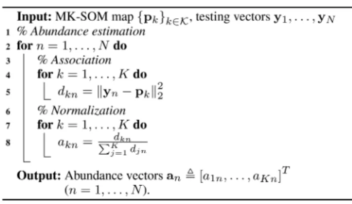
Following the ideas of [29, 31], we adopt an online implementation of MK-SOM algorithm detailed in Algorithm 1 (see Fig. 1). The

standard (i.e. affectation and representation) steps of the conventional SOM are iteratively applied here for a given total number T of epochs. In particular, the affectation step consists in finding the index kp of the so-called best-matching unit, i.e. of the

closest prototype pm of the considered input data xp. Note that the

MK-counterpart of SOM relies on a distance computed in the feature space ℍ thanks to the associated Gram matrix. Line 8 of Algorithm 1 (Fig. 1), the updating rule involves a neighbourhood function h ⋅ , ⋅ chosen as

h(t)_{m, m′ = exp −}∥ pm− pm′∥2

2σ2(t) (10)

where σ2(t) _{is an algorithmic parameter decreasing along with the}

iterations according to

σ2(t)_{= σ}2(t− 1)_{exp( − λ}

σ2t) (11)

with σ2(0)_{= 20 and λ}

σ2= 0.05. Moreover, μ(t) is a learning rate

defined as a decreasing function

μ(t)_{= μ}(t− 1)_{exp( − λ}

μt) (12)

with μ(0)_{= 0.1 and λ}

μ= 0.05. Finally, the δ( ⋅ ) function stands for

the Kronecker operator, i.e. δ(j) = 1 if j = 0 and δ(j) = 0

otherwise. In the proposed implementation, the output weight

vectors are normalised between the range (0, 255) as the input training and testing vectors have been also normalised [32].

It is worth noting that the output prototypes recovered during this training step can be interpreted as virtual endmember spectra or class representatives for each material present in the observed scene.

2.3 MK-SOM testing

The MK-SOM testing step of the proposed unmixing algorithm aims at recovering the abundance vector associated with each pixel

yn (n = 1, …, N) of the image to be unmixed. Following a

commonly accepted approach [20, 33, 34], the degrees of membership dkn kK= 1 of a testing pixel yn to all neurons pm are

resorted as surrogates of abundances. As in [20], these degrees are finally rescaled to ensure that the final abundance vectors satisfy the widely admitted non-negativity and sum-to-one constraints [2]. The overall process is described in Algorithm 2 (see Fig. 2).

2.4 Initialisation

Before beginning the unmixing process, two initialisation tasks should be conducted. There are discussed in what follows. First, the spectral signatures of the endmembers to be used in the unmixing process, as well as their number, should be selected. These spectral signatures can be chosen by the practitioner in the case of reliable prior knowledge regarding the scene of interest. Otherwise, one may make use of an endmember extraction algorithm already proposed in the literature [35–38]. Note that, as highlighted in [7, 8], some of these algorithms can provide reliable results to recover endmember from non-linearly mixed pixels, although they initially rely on an implicit LMM. This is, in particular, the case for the geometrical extraction algorithms, such as VCA [12] and N-FINDR [9]. Moreover, note that, in the proposed implementation of the MK-SOM, the number of endmembers is the squared value of the dimension of the SOM weight vectors. However, when this constraint can be fulfilled, any dimension of the SOM weight vectors can be still employed and the resulted map can be post-processed by any unsupervised clustering algorithm (e.g. K-means) to reach the desired number of endmembers [39].

Then, the second task consists in selecting training samples (i.e. hyperspectral pixels) necessary for the training step of the MKL. In [20, 40], the authors propose to resort to only pure pixels in the training phase, based on the assumption that each pure pixel can be associated with a unique endmember by a degree of membership equals to 1 and with a degree of membership to the other endmembers equal to 0. Instead, in this work, we propose to define this training set as the outputs of an endmember extraction algorithm, e.g. VCA. Indeed, VCA is able to recover the P most distinct pixels in the considered hyperspectral image. In addition to being unsupervised, this strategy has the great advantage of allowing the learning step of the MK-SOM to be conducted more efficiently since the training set is not limited to actual existing pure pixels in the image. In other words, the training pixels are selected as the P purest pixels extracted by VCA.

3 Experimental results

To validate the proposed MK-SOM-based unmixing algorithm, its performance has been compared to those obtained by the linear unmixing methods FCLS [13] and SUNSAL [14] and the non-linear unmixing methods PPNM [16], rLMM [18], K-Hype and its generalised counterpart (SK-Hype) [41]. The experimental datasets consist of synthetic and real images described in what follows.

3.1 Datasets

Firstly, to assess the performance of the unmixing procedures, we consider a hyperspectral image of size 100 × 100 pixels and composed of nine endmembers representative of minerals which have been extracted from the U.S. Geological Survey (USGS) spectral library [42]. The abundance maps have been choosing as

Fig. 1  Algorithm 1: MK-SOM unmixing: training step

freely available dataset referred to as Fractal 1 and available online [43] has been used. They have been generated according to fractal patterns to ensure realistic distribution of the materials other the scene. In particular, it is constructed such that the pixels nearby the region centres are more spectrally pure than the pixels in the transition areas [44]. Based on these endmembers and abundance maps, the mixed pixels have been generated according to the non-linear model, namely the so-called Fan binon-linear model introduced in [45]. An additive white Gaussian noise has been considered with a corresponding signal-to-noise ratio chosen as SNR=40 dB. To illustrate Fig. 3 depicts the synthetic image in a band _#1.

Secondly, the real so-called Cuprite dataset acquired by the airborne visible/infrared imaging spectrometer (AVIRIS) has been considered [46]. It consists of a 614 × 512 pixel image and 224 bands with a spectral range of 0.4 − 2.5 μm. A set of 33 bands have been removed prior to analysis since they correspond to water absorption band or low SNR. Fig. 4 shows the Cuprite image observed in band #10.

3.2 Quality metrics

For the synthetic dataset for which ground-truth (i.e. in terms of actual abundance maps) is available, the performances of the unmixing procedures are evaluated through the mean square error of the abundances [47] MSEA= 1_NK

∑

where an and a^n are the actual and estimated abundance vectors

associated with the pixel #n (n ∈ 1, …, N ), respectively, and K is the number of endmembers used during the unmixing process.

For the real datasets for which no ground-truth is available, the reconstruction error between the original and recovered pixel signatures [47] REY= 1_LN

∑

where yn and y^n are the measured and reconstructed spectra

associated with the pixel #n (n ∈ 1, …, N ) and L is the number of spectral bands.

3.3 Results

In the conducted experiments, the proposed MK-SOM unmixing procedure has been implemented with a Gaussian kernel of width equal to 1 since it has shown to outperform linear and polynomial kernels [26]. During the training step, various numbers T_epoch of epochs have been considered T_epoch∈ 20, 35, 50, 100, 200, 500 with the largest size of training sets, which equals the number of bands.

Tables 1 and 2 report the performance of the different considered algorithms for a number of endmembers equal to K = 4

and _{K = 9, respectively and an SNR = 40 dB. These results show} that, in the case of a number of endmembers equal to 4, the proposed MK-SOM unmixing algorithm consistently outperforms all the other algorithms for any training step parameters (e.g. number Tepoch of epochs). The best MSE value (0.0625) is obtained

by MK-SOM for a number of epochs equals to T_epoch= 500. When the number of endmembers is equal to K = 9, the MK-SOM

consistently performs better than all other methods. The best MSE value (0.0123) is reached when MK-SOM is run with the number of epochs equal to Tepoch= 500.

To illustrate, the corresponding estimated abundance maps for a synthetic image are depicted in Fig. 5 for _{K = 4.}

As complementary results, Figs. 6 and 7 report the reconstruction errors for different levels of noise for K = 4 and a

different number of endmembers for SNR = 40, respectively. Similarly, Table 3 shows the performance of compared algorithms when applied to the real AVIRIS Cuprite dataset for a number of endmembers equal to K = 9. The proposed MK-SOM

consistently outperforms the concurrent methods and, in particular, provides the lowest error for a number of epochs equal to

T_epoch= 20. To illustrate, the corresponding estimated abundance

maps are depicted in Fig. 8 for K = 4.

4 Parallel implementation of the MK-SOM

algorithm

This section presents a parallel implementation of the MK-SOM algorithm described in Section 2. This implementation is developed on a GPU using a CUDA programming language. The experiments are conducted on an NVidia Tesla N2090 architecture and show that the parallelisation provides a significant speedup of the required computational time. Per se, MK-SOM learning is a highly parallelised problem as it is based on an SOM learning approach. The complexity of the calculation is greatly affected by the SOM map size and number of features (number of bands in the

Fig. 3  Band _{#1 of the synthetic image}

Fig. 4  Band #10 of the AVIRIS Cuprite image

Table 1 Synthetic dataset (_{K = 4): estimated abundance}

MSE FCLS 0.0982 SUNSAL 0.1039 PPNM 0.1013 rLMM 0.0982 K-Hype 0.0977 SK-HYPE 0.1010 MK-SOM Tepoch 20 0.0626 35 0.0626 50 0.0626 100 0.0626 200 0.0625 500 0.0625

Table 2 Synthetic dataset (_{K = 9): estimated abundance}

MSE FCLS 0.0190 SUNSAL 0.0192 PPNM 0.0189 rLMM 0.0189 K-Hype 0.0181 SK-HYPE 0.0185 MK-SOM Tepoch 20 0.0123 35 0.0123 50 0.0123 100 0.0124 200 0.0123 500 0.0123

considered unmixing problem). A simple SOM learning can be summarised as Algorithm 3 (see Fig. 9).

The most computationally intensive steps are Steps 3 and 4 of Algorithm 3 (Fig. 9) described below:

• Computing the Euclidean distance between the selected training sample and the SOM map, then obtaining the best matching unit (BMU) which correspond to the minimum distance,

• Updating the SOM map weights according to the distance between the selected training sample and BMU yet updates are limited to only the BMU neighbours.

The degree of parallelism of Step 3 is limited to the dimension of the training set (number of features). On the other hand, the complexity of the MK-SOM testing step (see Section 2.3 and Algorithm 2 (Fig. 2)) mainly depends on the image size, the SOM map size and the number of endmembers. Therefore, for a given image, the expected parallelisation speedup directly increases with the SOM map size. As an illustrative example of the possible computational gain, the implemented CUDA version has been evaluated in the real AVIRIS Cuprite Image of size 512 × 614 × 189 with different SOM map sizes. The resulting computational times, compared to those obtained on crude (i.e.

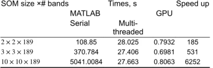
serial) or multi-threading MATLAB implementations, are reported in Table 4. These results show a significant speedup ranging from × 185 to × 6252 with respect to its MATLAB counterpart. It clear appears that this computation speedup increases as the SOM map size increases. We could also note that the execution time of the serial MATLAB version is exponentially increasing with SOM map size.

5 Conclusion

This paper introduced a new unmixing method based on simple MKL with SOM as a solver. The proposed non-linear unmixing approach succeeded in reducing the estimation error when applied to synthetic and real hyperspectral images. Moreover, it seemed to be robust with respect to the choice of the parameters required by

Fig. 5  Synthetic dataset (K = 4): estimated abundance maps. From top to bottom: FCLS, SUNSAL, PPNM, rLMM, K-Hype, SK-Hype, proposed MK-SOM method. For the proposed MK-MK-SOM algorithm, the abundance maps have been estimated with a Tepoch= 500

Fig. 6  Synthetic dataset (K = 4): RMSE for SNR ∈ 20, 40, 60, 80

Fig. 7  Synthetic dataset (_{SNR = 40): RMSE for K ∈ 4, 6, 8, 9}

Table 3 Real AVIRIS Cuprite dataset (_{K = 9):}

reconstruction error FCLS 3.0208 SUNSAL 3.3709 PPNM 2.9808 rLMM 5.8459 K-Hype 3.0093 SK-HYPE 2.9263 MK-SOM Tepoch 20 2.1544 35 2.3510 50 2.3871 100 3.2251 200 3.2602 500 3.2603

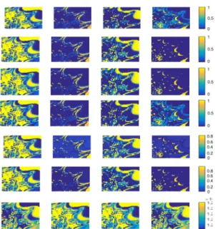
Fig. 8  Real AVIRIS Cuprite dataset (K = 4): estimated abundance maps. From top to bottom: FCLS, SUNSAL, PPNM, rLMM, K-Hype, SK-Hype, proposed MK-SOM method. For the proposed MK-SOM algorithm, the abundance maps have been estimated with a Tepoch= 20

the training stage. At the price of a slightly more computationally intensive complexity, the proposed MK-SOM framework appears as a relevant alternative of state-of-the-art non-linear unmixing methods. Finally, this paper showed that a parallel implementation of the proposed algorithm was possible. This parallelisation was implemented using a graphics processing unit and the resulting computational gain was shown to be highly significant when compared to serial and multi-threaded MATLAB implementations.

6 Acknowledgment

This work was funded by EU FP7 through the ERANETMED JC-WATER program, MapInvPlnt Project ANR-15-NMED-0002-02.

7 References

[1] Bioucas-Dias, J.M., Plaza, A., Camps-Valls, G., et al.: ‘Hyperspectral remote sensing data analysis and future challenges’, IEEE Geosci. Remote Sens.

Mag., 2013, 1, (2), pp. 6–36

[2] Bioucas-Dias, J.M., Plaza, A., Dobigeon, N., et al.: ‘Hyperspectral unmixing overview: geometrical, statistical, and sparse regression-based approaches’,

IEEE J. Sel. Top. Appl. Earth Obs. Remote Sens., 2012, 5, pp. 354–379

[3] Dobigeon, N., Tits, L., Somers, B., et al.: ‘A comparison of nonlinear mixing models for vegetated areas using simulated and real hyperspectral data’, IEEE

J. Sel. Top. Appl. Earth Obs. Remote Sens., 2014, 7, pp. 1869–1878

[4] Meganem, I., Déliot, P., Briottet, X., et al.: ‘Linear-quadratic mixing model for reflectances in urban environments’, IEEE Trans. Geosci. Remote Sens., 2014, 52, pp. 544–558

[5] Hapke, B.: ‘Theory of reflectance and emittance spectroscopy’ (Cambridge Univ. Press, Cambridge, UK, 1993)

[6] Heylen, R., Parente, M., Gader, P.: ‘A review of nonlinear hyperspectral unmixing methods’, IEEE J. Sel. Top. Appl. Earth Obs. Remote Sens., 2014,

7, pp. 1844–1868

[7] Dobigeon, N., Tourneret, J.-Y., Richard, C., et al.: ‘Nonlinear unmixing of hyperspectral images: models and algorithms’, IEEE Signal Process. Mag., 2014, 31, pp. 82–94

[8] Dobigeon, N., Altmann, Y., Brun, N., et al.: ‘Linear and nonlinear unmixing in hyperspectral imaging’, in Ruckebusch, C. (Ed.): ‘Resolving spectral

mixtures – with application from ultrafast time-resolved spectroscopy to superresolution imaging’, Data Handling in Science and Technology, vol. 30,

(Elsevier, Oxford, UK, 2016), pp. 185–224

[9] Winter, M.E.: ‘N-FINDR: an algorithm for fast autonomous spectral end-member determination in hyperspectral data’. Proc. SPIE Imaging Spectrometry V, Denver, USA, 1999, vol. 3753, pp. 266–275

[10] Chang, C.-I., Wu, C.-C., min Liu, W., et al.: ‘A new growing method for simplex-based endmember extraction algorithm’, IEEE Trans. Geosci.

Remote Sens., 2006, 44, (10), pp. 2804–2819

[11] Boardman, J.W.: ‘Automating spectral unmixing of AVIRIS data using convex geometry concepts’. Summaries 4th Annual JPL Airborne Geoscience Workshop, Washington, D.C., 1993, vol. 1, pp. 11–14

[12] Nascimento, J.M., Dias, J.M.B.: ‘Vertex component analysis: a fast algorithm to unmix hyperspectral data’, IEEE Trans. Geosci. Remote Sens., 2005, 43, (4), pp. 898–910

[13] Heinz, D.C., Chang, C.-I.: ‘Fully constrained least squares linear spectral mixture analysis method for material quantification in hyperspectral imagery’,

IEEE Trans. Geosci. Remote Sens., 2001, 39, (3), pp. 529–545

[14] Bioucas-Dias, J.M., Figueiredo, M.A.: ‘Alternating direction algorithms for constrained sparse regression: application to hyperspectral unmixing’. Proc. IEEE GRSS Workshop Hyperspectral Image Signal Processing: Evolution in Remote Sensing (WHISPERS), Reykjavik, Iceland, 2010, pp. 1–4

[15] Altmann, Y., Dobigeon, N., Tourneret, J.-Y.: ‘Bilinear models for nonlinear unmixing of hyperspectral images’. Proc. IEEE GRSS Workshop Hyperspectral Image Signal Processing: Evolution in Remote Sensing (WHISPERS), Lisbon, Portugal, June 2011, pp. 1–4

[16] Altmann, Y., Halimi, A., Dobigeon, N., et al.: ‘Supervised nonlinear spectral unmixing using a postnonlinear mixing model for hyperspectral imagery’,

IEEE Trans. Image Process., 2012, 21, (6), pp. 3017–3025

[17] Altmann, Y., Dobigeon, N., Tourneret, J.-Y.: ‘Unsupervised post-nonlinear unmixing of hyperspectral images using a Hamiltonian Monte Carlo algorithm’, IEEE Trans. Image Process., 2014, 23, pp. 2663–2675

[18] Févotte, C., Dobigeon, N.: ‘Nonlinear hyperspectral unmixing with robust nonnegative matrix factorization’, IEEE Trans. Image Process., 2015, 24, pp. 4810–4819

[19] Halimi, A., Bioucas-Dias, J., Dobigeon, N., et al.: ‘Fast hyperspectral unmixing in presence of nonlinearity or mismodelling effects’, IEEE Trans.

Comput. Imaging, 2017, 3, pp. 146–159

[20] Licciardi, G.A., Frate, F.D.: ‘Pixel unmixing in hyperspectral data by means of neural networks’, IEEE Trans. Geosci. Remote Sens., 2011, 49, (11), pp. 4163–4172

[21] Ayerdi, B., Graña, M.: ‘Hyperspectral image nonlinear unmixing and reconstruction by elm regression ensemble’, Neurocomputing, 2016, 174, pp. 299–309

[22] Gönen, M., Alpaydın, E.: ‘Multiple kernel learning algorithms’, J. Mach.

Learn. Res., 2011, 12, pp. 2211–2268

[23] Sonnenburg, S., Rätsch, G., Schäfer, C., et al.: ‘Large scale multiple kernel learning’, J. Mach. Learn. Res., 2006, 7, pp. 1531–1565

[24] Liu, K.-H., Lin, Y.-Y., Chen, C.-S.: ‘Linear spectral mixture analysis via multiple-kernel learning for hyperspectral image classification’, IEEE Trans.

Geosci. Remote Sens., 2015, 53, (4), pp. 2254–2269

[25] Chen, J., Richard, C., Honeine, P.: ‘Nonlinear unmixing of hyperspectral images based on multi-kernel learning’. Proc. IEEE GRSS Workshop Hyperspectral Image Signal Processing: Evolution in Remote Sensing (WHISPERS), Shanghai, China, 2012

[26] Gu, Y., Wang, S., Jia, X.: ‘Spectral unmixing in multiple-kernel Hilbert space for hyperspectral imagery’, IEEE Trans. Geosci. Remote Sens., 2013, 51, (7), pp. 3968–3981

[27] Kohonen, T., Somervuo, P.: ‘Self-organizing maps of symbol strings’,

Neurocomputing, 1998, 21, (1), pp. 19–30

[28] Martínez, P., Gualtieri, J., Aguilar, P., et al.: ‘Hyperspectral image classification using a self-organizing map’. Summaries of the X JPL Airborne Earth Science Workshop, Pasadena, USA, 2001

[29] Olteanu, M., Villa-Vialaneix, N., Cierco-Ayrolles, C.: ‘Multiple kernel selforganizing maps’. European Symp. Artificial Neural Networks, Computational Intelligence Machine Learning, Bruges, Belgium, 2013, p. 83 [30] MacDonald, D., Fyfe, C.: ‘The kernel self-organising map’. Proc. 4th Int.

Conf. on Knowledge-Based Intelligent Engineering Systems and Allied Technologies, Salt Lake City, USA, 2000, vol. 1, pp. 317–320

[31] Villa-Vialaneix, N., Rossi, F.: ‘A comparison between dissimilarity SOM and kernel SOM for clustering the vertices of a graph’. Proc. Workshop on Self-Organizing Maps (WSOM), Bielefeld, Germany, 2007, p. WeP–1

[32] Blayo, F.: ‘Kohonen self-organizing maps: is the normalization necessary?’,

Complex Syst., 1992, 6, (6), pp. 105–123

[33] Guilfoyle, K.J., Althouse, M.L., Chang, C.-I.: ‘A quantitative and comparative analysis of linear and nonlinear spectral mixture models using radial basis function neural networks’, IEEE Trans. Geosci. Remote Sens., 2001, 39, pp. 2314–2318

[34] Altmann, Y., Dobigeon, N., McLaughlin, S., et al.: ‘Nonlinear unmixing of hyperspectral images using radial basis functions and orthogonal least squares’. Proc. IEEE Int. Conf. Geoscience Remote Sensing (IGARSS), Vancouver, Canada, July 2011, pp. 1151–1154

[35] Chang, C.-I., Du, Q.: ‘Estimation of number of spectrally distinct signal sources in hyperspectral imagery’, IEEE Trans. Geosci. Remote Sens., 2004,

42, (3), pp. 608–619

[36] Wang, J., Chang, C.-I.: ‘Applications of independent component analysis in endmember extraction and abundance quantification for hyperspectral imagery’, IEEE Trans. Geosci. Remote Sens., 2006, 44, (9), pp. 2601–2616 [37] Wang, J., Chang, C.-I.: ‘Independent component analysis-based

dimensionality reduction with applications in hyperspectral image analysis’,

IEEE Trans. Geosci. Remote Sens., 2006, 44, (6), pp. 1586–1600

[38] Plaza, A., Chang, C.-I.: ‘Impact of initialization on design of endmember extraction algorithms’, IEEE Trans. Geosci. Remote Sens., 2006, 44, (11), pp. 3397–3407

[39] Vesanto, J., Alhoniemi, E.: ‘Clustering of the self-organizing map’, IEEE

Trans. Neural Netw., 2000, 11, (3), pp. 586–600

[40] Foody, G.M.: ‘Relating the land-cover composition of mixed pixels to artificial neural network classification output’, Photogramm. Eng. Remote

Sens., 1996, 62, (5), pp. 491–498

[41] Chen, J., Richard, C., Honeine, P.: ‘Nonlinear unmixing of hyperspectral data based on a linear-mixture/nonlinear-fluctuation model’, IEEE Trans. Signal

Process., 2013, 61, (2), pp. 480–492

[42] ‘USGS digital spectral library’. Available at http://speclab.cr.usgs.gov/ spectral-lib.html, accessed 17 June 2016

[43] ‘HyperMIX: ground truth for fractal images’. Available at http:// hypercomp.es/hypermix/node/585, accessed 17 June 2016

[44] Martín, G., Plaza, A.: ‘Region-based spatial preprocessing for endmember extraction and spectral unmixing’, IEEE Geosci. Remote Sens. Lett., 2011, 8, (4), pp. 745–749

[45] Fan, W., Hu, B., Miller, J., et al.: ‘Comparative study between a new nonlinear model and common linear model for analysing laboratory simulated-forest hyperspectral data’, Int. J. Remote Sens., 2009, 30, (11), pp. 2951–2962

[46] ‘Hyperspectral remote sensing scenes’. Available at http://www.ehu.eus/ ccwintco/index.php?title=Hyperspectral Remote Sensing Scenes, accessed 1 February 2016

[47] Plaza, J., Plaza, A., Martínez, P., et al.: ‘H-COMP: A tool for quantitative and comparative analysis of endmember identification algorithms’. Proc. IEEE Int. Conf. Geoscience Remote Sensing (IGARSS), Toulouse, France, 2003, vol. 1, pp. 291–293

Table 4 Real AVIRIS Cuprite dataset: comparison of

computational times

SOM size ×# bands Times, s Speed up MATLAB GPU Serial Multi-threaded 2 × 2 × 189 108.85 28.025 0.7932 185 3 × 3 × 189 370.784 27.406 0.6981 531 10 × 10 × 189 5041.0084 27.663 0.8063 6252