Open Archive TOULOUSE Archive Ouverte (OATAO)
OATAO is an open access repository that collects the work of Toulouse researchers and
makes it freely available over the web where possible.
This is an author-deposited version published in :
http://oatao.univ-toulouse.fr/
Eprints ID : 14321
To link to this article : DOI :10.1109/TSP.2015.2460218
URL :
http://dx.doi.org/10.1109/TSP.2015.2460218
To cite this version : Abramovich, Yuri and Besson, Olivier and
Johnson, Ben
Bounds for maximum likelihood regular and
non-regular DoA estimation in K-distributed noise.
(2015)
IEEE Transactions on Signal Processing, vol. 63 (n° 21). pp. 5746 -
5757. ISSN 1053-587X
Any correspondance concerning this service should be sent to the repository
administrator:
[email protected]
Bounds for Maximum Likelihood Regular and
Non-Regular DoA Estimation in
-Distributed Noise
Yuri I. Abramovich, Fellow, IEEE, Olivier Besson, Senior Member, IEEE, and Ben A. Johnson, Senior Member, IEEE
Abstract—We consider the problem of estimating the direction
of arrival of a signal embedded in -distributed noise, when sec-ondary data which contains noise only are assumed to be avail-able. Based upon a recent formula of the Fisher information ma-trix (FIM) for complex elliptically distributed data, we provide a simple expression of the FIM with the two data sets framework. In the specific case of -distributed noise, we show that, under cer-tain conditions, the FIM for the deterministic part of the model can be unbounded, while the FIM for the covariance part of the model is always bounded. In the general case of elliptical distributions, we provide a sufficient condition for unboundedness of the FIM. Accurate approximations of the FIM for -distributed noise are also derived when it is bounded. Additionally, the maximum likeli-hood estimator of the signal DoA and an approximated version are derived, assuming known covariance matrix: the latter is then es-timated from secondary data using a conventional regularization technique. When the FIM is unbounded, an analysis of the estima-tors reveals a rate of convergence much faster than the usual . Simulations illustrate the different behaviors of the estimators, de-pending on the FIM being bounded or not.
Index Terms—Direction of arrival estimation, distributed
noise, Cramér-Rao bounds, maximum likelihood estimation.
I. PROBLEMSTATEMENT
E
STIMATING THE DIRECTION OF ARRIVAL (DoA) of multiple signals impinging on an array of sensors from observation of a finite number of array snapshots has been ex-tensively studied in the literature [1]. Maximum likelihood es-timators (MLE) and Cramér-Rao bounds (CRB), derived under the assumption of additive white Gaussian noise, and either for the so-called conditional or unconditional model [2]–[5], serve as references to which newly developed DoA estimators have been systematically compared. In many instances however, ad-ditive noise is usually colored and, consequently, the problemManuscript received March 24, 2015; revised June 18, 2015; accepted July 15, 2015. Date of publication July 23, 2015; date of current version September 30, 2015. The associate editor coordinating the review of this manuscript and approving it for publication was Prof. Lei Huang. The work of O. Besson is supported by DGA/MRIS under grant no. 2012.60.0012.00.470.75.01.
Y. I. Abramovich is with W. R. Systems, Ltd., Fairfax, VA 22030 USA (e-mail: [email protected]).
O. Besson is with the University of Toulouse, ISAE-Supaéro, De-partment Electronics Optronics Signal, 31055 Toulouse, France (e-mail: [email protected]).
B. A. Johnson is with the University of South Australia—ITR, Mawson Lakes SA 5085, Australia (e-mail: [email protected]).
of DoA estimation in spatially correlated noise fields has been studied, see e.g., [6]–[10].
When the spatial covariance matrix of this additive noise is known a priori, maximum likelihood estimators and Cramér-Rao bounds are changing in a straightforward way with whitening operations. The new statistical problem ap-pears when the covariance matrix of the additive noise is not known a priori and information about this matrix is substi-tuted by a number of independent and identically distributed (i.i.d.) training samples, that form the so-called secondary training sample data set. In many cases one can assume that the statistical properties of the training noise data are the same as per noise data within the primary training set data: such conditions are usually referred to as the supervised training conditions. Therefore, under these conditions, one has two sets of measurements, one primary set which contains signals of interest (SOI) and noise, and a second set
(secondary training set) which contains noise only. Examples of this problem formulation are numerous in the area of passive location and direction finding. For instance, in the so-called over-sampled 2D HF antenna arrays, ionospherically propagated external noise is spatially non white [11], [12], and some parts of HF spectrum (distress signals for example) with no signals may be used for external noise sampling [13]. Despite its relevance in many practical situations, this problem has been relatively scarcely studied [14], [15]. For parametric description of the Gaussian noise covariance matrix with the unknown parameter vector, in [15], the authors derive the Cramér-Rao bound for joint SOI parameters (DoA) and noise parameters estimation, assuming a conventional uncon-ditional model, i.e.,
and where stands for the complex Gaussian distribution whose respective parameters are the mean, row covariance matrix and column covariance matrix. is the usual steering matrix with the vector of unknowns DoA, denotes the waveforms covariance matrix and corresponds to the noise covariance matrix, which is parameterized by vector .
In many cases however, the Gaussian assumption for the pre-dominant part of the noise cannot be advocated. Typical ex-ample is the HF external noise, heavily dominated by pow-erful lighting strikes [16]–[18]. Evidence of deviations from the Gaussian assumption has been demonstrated numerous times for different applications, with the relevance of the compound-Gaussian (CG) models being justified [19]–[24]. In essence, the individual -variate snapshot of such a noise over the face of an antenna array may be treated as a Gaussian random vector, whose power can randomly fluctuate from sample to sample. CG models belong to a larger class of distributions, namely mul-tivariate elliptically contoured distributions (ECD) [25]–[27].
For the sake of clarity, we briefly review the main definitions of ECD. A vector follows an EC distribution if it ad-mits the following stochastic representation
(1) where means “has the same distribution as”. In (1), is a non-negative real random variable and is independent of the complex random vector which is uniformly distributed over the complex sphere . The matrix is such that where is the so-called scatter ma-trix, and we assume here that is non-singular. The probability density function (p.d.f.) of can then be written as
(2) where stands for proportional to. The function
is called the density generator and satisfies finite moment condition . It is related to the p.d.f. of the modular variate by .
Going back to our scenario of two data sets
and , we assume that they are independent, and that their columns are inde-pendent and identically distributed (i.i.d.) according to (2). In other words, one has and , where and are i.i.d. variables drawn from , and and are i.i.d. random vectors uniformly distributed on the unit sphere. It then follows that the joint distribution of is given
by where
and
(3a)
(3b) where . Additionally, we assume that de-pends on a parameter vector while depends on . Our objective is then to estimate
from . Let us emphasize an essential difference of the problem in (3) with respect to the typical problem of target detection in CG clutter [28]. There, within each range reso-lution cell the clutter is perfectly Gaussian and therefore the optimum space-time processing is the same as per the stan-dard Gaussian problem formulation. It is the data dependent threshold and clutter covariance matrix (in adaptive formula-tion) that needs to be calculated from the secondary data, if not known a priori [28], [29]. In the problem (3), the SOI DoA es-timation should be performed on a number of ECD i.i.d. pri-mary training samples, and maximum likelihood DoA estima-tion algorithm and CRB should be expected to be very different from the Gaussian case.
The paper is organized in the following way. In Section II, we derive a general expression of the FIM for elliptically dis-tributed noise using two data sets. Section III focuses on the case
of DoA estimation in -distributed noise. In Section III.B, we derive conditions under which the FIM is bounded/unbounded, and provide a sufficient condition for unboundedness of the FIM with general elliptical distribution. The maximum like-lihood estimate, as well as an approximation, are derived in Section III.C. In the same section, we derive lower and upper bounds on the mean-square error of the MLE for non-regular estimation conditions, i.e., when the Fisher information matrix is unbounded. Numerical simulations serve to evaluate the per-formance of the estimators in Section IV and our conclusions are drawn in Section V.
II. CRAMÉR-RAOBOUNDS
In this section, we derive the CRB for estimation of parameter vector from the distribution in (3). The Fisher information matrix (FIM) for the problem at hand can be written as [1]
(4) where we used the fact that
(5) Hence, the total FIM is the sum of two matrices , with straightforward definition from (4). In order to derive each matrix, we will make use of the general expression of the Fisher information matrix for ECD recently derived in [30], [31]. First, let us introduce
(6) where . Then, we have from [30] that the -th element of the Fisher information matrices is given by
(7)
(8) where . Since depends only on , it follows that
takes the following form
with
(10) where . Let us now consider . Using the fact that depends only on and depends only on is block-diagonal, i.e.,
(11) with
(12a)
(12b) The whole FIM is thus given by
(13) The CRB for estimation of is obtained as the upper-left block of the inverse of the FIM and is thus simply . Similarly to the Gaussian case, the CRB for estimation of in the conditional model is the same as if was known. As for the CRB for estimation of , it is the same as if we had a set of noise only samples.
III. APPLICATION TO -DISTRIBUTEDNOISE
A. Data Model
We address the specific problem where the primary data can be written as
(14) where follows a Gamma distribution with shape parameter
and scale parameter , i.e., its p.d.f. is given by
(15) which we denote as , and . The noise component is known to follow a distribution and in (14) admits a representation similar to (1) with
. The p.d.f. of in this case is given by
(16)
where is the modified Bessel function. Note that the -th order moment of is
(17) where we used the fact ([32], 6.656.16) that
(18) The density generator is thus here
(19) where, for the sake of notational convenience, we have dropped the subscript .
B. Cramér-Rao Bounds
The FIM for -distributed noise can be obtained from the FIM for Gaussian distributed noise and the calculation of the scalar
(20) for . For the signal parameters part only, we indeed have where the subscript and stand for -distributed and Gaussian distributed noise. Using the fact that , it follows that
(21) It then ensues that
and thus
(23) A formula for the FIM in case of -distributed noise was de-rived in [33] based on the compound Gaussian representation (14). While it resembles our derivations based on the FIM for ECD derived in [30], it does not match exactly our expression herein. Moreover, we study herein the existence of the FIM and derive a closed-form approximation of the FIM.
Let us investigate the conditions under which the integral (24) converges. Towards this end, let us use the following inequality which holds for and [34]
(25) It follows that
(26) The first integral converges for
while the second converges for . Hence, for , one has
(27) Additionally, one has, for
(28)
which implies that
(29) The first integral converges for and the second converges for . In the former case, one has
(30) Consequently, we conclude that the integral converges only for : for this implies that which is verified. In contrast, when , one must have . In other words, the term in the FIM corresponding to the noise
parameters is always bounded since it depends on only. The
situation is different for signal parameters. In an unconditional model where would depend on signal parameters as well, the FIM is bounded. In contrast, in the conditional model where signal parameters are embedded in the mean of the distribution, the FIM corresponding to signal parameters is bounded only for : otherwise, it is unbounded. The latter case corresponds to the so-called non regular case corresponding to distributions with singularities, as studied e.g., in [35].
Before pursuing our study of the FIM for the specific case of -distributed noise, let us make an important observation. For the distribution, we have just proven that does not exist for
. However, see (17), exists if and only if and . The latter condition implies that, when
does not exist. Observe that convergence of the latter integral is problematic in a neighborhood of 0, since for
as is a density. Therefore, at least for -distributed noise, if does not exist, then is unbounded. At this stage, one may wonder if this property extends to any other elliptical distribution. It turns out that this is indeed the case, as stated and proved in the next proposition.
Proposition 1: Whatever the p.d.f. of the modular variate
, if then .
Proof: For the sake of notational convenience, we
tem-porarily omit the subscript and use instead of . Let us first observe that
(31) Since , one can write
which implies that
(33) Therefore
(34) The third term of the sum is always positive. In the second term, we have that . It follows that divergence of is a sufficient condition for divergence of
. As said before
exists, and therefore a sufficient condition for to be undounded is that is unbounded.
Let us now go back to the -distributed case and investigate whether it is possible to derive a simple expression for and subsequently , assuming that . Towards this end, let us make use of
(35) to write that
(36)
The last term is obviously not possible to obtain in closed-form so that we use a “large ” approximation of the modified Bessel function (37) which results in (38) Therefore, (39) We finally have (40) If the large approximation is made from the start, then one has (41) so that (42) and hence (43)
Fig. 1 compares the approximations in (40) and (43), as well as a method which uses random number generation to approxi-mate based on its initial definition in (20). More precisely, we generated a large number of random variables
and replace the statistical expectation of (20) by an av-erage over the so-generated random variables. As can be ob-served from Fig. 1, the 3 approximations provide very close values, which enable one to validate the closed-form expres-sions in (40) and (43).
C. Maximum Likelihood Estimation
We now focus on maximum likelihood (ML) estimation of direction of arrival , signal waveforms and covariance matrix in the model
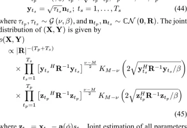
(44) where , and . The joint distribution of is given by
(45) where . Joint estimation of all parameters appears to be very complicated and hence we will proceed in two steps. At first, we assume that is known and derive the ML estimates of and . Then, is substituted for some estimate obtained from observation of only.
1) DoA Estimation With Known : Assuming that is
known, one needs to maximize with respect to and
(46) where is given by (19). Since is monotonically de-creasing, see (21), it follows that is maximized when the argument of is minimized. However,
(47) Therefore, for any is maximized when
(48) It ensues that one needs now to maximize, with respect to
(49)
Fig. 1. Comparison of the approximations of in (40) and (43). and .
with . In order to avoid calcula-tion of a modified Bessel funccalcula-tion and thus in order to simplify estimation, we propose to make use of the “large ” approx-imation of the modified Bessel function given in (37) to write
(50) This approximation results in an approximate maximum likeli-hood (AML) estimator of which consists in maximizing
(51) Note that
(52) which should be compared to the concentrated log likelihood function in the Gaussian case, as given by
(53)
A few remarks are in order about these estimates, in partic-ular about the behavior of the AML estimator in the case of un-bounded FIM, i.e., when . First, note that all estimates will be a function of
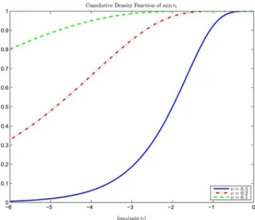
Fig. 2. Cumulative density function of . and .
where is the projection onto the orthogonal com-plement of . Compared to (53), the logarithm oper-ation in (51) will strongly emphasize those snapshots for which is small. Let us thus investigate the properties of this statistic, when evaluated at the true value of signal DOA . Using the fact that , where and is a short-hand notation for
, one has
(55) For small , it follows that, in the vicinity of , the snapshot with minimal is more or less the snapshot for which is minimum, hence the snapshot for which noise power is minimum, which makes sense. If we let , then its cumulative density function (c.d.f.) is given by
(56) which is shown in Fig. 2. Obviously, with small , the snapshot which corresponds to the minimum value of exhibits a very high signal to noise ratio and, due to the emphasizing effect of the operation in (51), the performance of the AML estimator is likely to be driven mainly by this particular snapshot. This is illustrated in Fig. 3 where we display the mean-square error (MSE) of the AML estimate which uses all snapshots and the MSE of an hypothetical AML estimator which would use only the snapshot corresponding to the minimum value of . The scenario of this simulation is described in the next section. This figure shows a marginal loss of the AML estimator using only, as compared to the full AML estimator, especially for small .
Let us thus analyze the behavior of the AML estimators. For the sake of notational convenience, let and denote the AML estimator using snapshots with -distributed noise and the AML estimator using the snapshot corresponding
Fig. 3. Mean square error of AML estimator using either all snapshots or a single snapshot corresponding to minimal . known, and
dB.
to the minimal , respectively. Observe that, when using a single snapshot , minimizing (51) is equivalent to mini-mizing the Gaussian likelihood function in (53) with . Since exhibits a high signal to noise ratio, is close to , one can make a Taylor expansion and relate the error
to the error as
(57) where is some vector that depends essentially on the deriva-tives of [36] and whose expression is not needed here. One can simply notice that would be the same with Gaussian noise and a single snapshot, since maximizing (51) or (53) is equiva-lent when one snapshot is used. This implies that
(58) Observe that is the mean-square error (MSE) that would be obtained in Gaussian noise and a single snapshot, which is about times the MSE obtained in the Gaussian case and using snapshots, and the latter is approximately the Gaussian CRB. The MSE of depends on where is the minimum value of a set of independent and identically dis-tributed (actually gamma disdis-tributed) variables. Therefore, in order to obtain , one must consider statistics of extreme values, a field that has received considerable attention for a long time, see e.g., [37]–[39]. It turns out that only asymptotic (as ) results are available and we build upon them to de-rive the rate of convergence of . First, note that
Now since is small and is large, is very small and we can approximate , which yields
(60) It follows from (60) that, asymptotically, the p.d.f. of
is approximately
(61) Using integration by parts, it follows that
(62) One can then conclude that, as goes to infinity,
(63) Therefore, in the case of , the MSE of de-creases as , a rate of convergence much faster than the usual . Note that this case corresponds to unbounded FIM. Such rates of convergence are also found with distributions pos-sessing singularities ([35], chapter 6).
As for the AML estimate obtained from snapshots, namely , its MSE is upper-bounded by that (since it uses all snapshots, including ), and is lower-bounded by the MSE that would be obtained if for , and this MSE is times the MSE of . Additionally, as said before, we have where is the Gaussian CRB using snapshots. Hence, one can bound the MSE of as
(64) As will be illustrated in the next section, the upper bound is rather tight, while the lower bound is much lower than the actual MSE.
2) Estimation of Using Secondary Data: When is not
known, then the secondary data can be used to estimate it. The maximum likelihood estimator is obtained (for )
as the solution (up to a scaling factor) to the following implicit equation [27]
(65)
can be obtained through an iterative procedure, whose convergence is guaranteed under the assumptions made [27]. In order to avoid evaluation of the modified Bessel function, one can use the large approximation of in (41) to define as the solution to the fixed-point solution
(66) Note that is more or less the well-known Tyler fixed-point estimator [40], which again can be obtained from an it-erative procedure whose convergence is guaranteed [29], [41]. The drawbacks of the two above estimators are that 1) they are suited to a distribution for the noise and 2) is required to be larger than . In order to gain robustness against these problems, a solution is to use normalized data
whose distribution is independent of that of the noise, and to use regularization. More precisely, we suggest to resort to the fol-lowing scheme [42]–[44]
(67a)
(67b)
and define since convergence of this iterative scheme has been proved [45]. The very good per-formance of this scheme has been illustrated in various appli-cations, see e.g., [43]–[47], where discussions on how to select the regularization parameter can also be found.
IV. NUMERICALSIMULATIONS
We assume a linear array of elements spaced a half-wavelength apart and we consider the simple scenario of a single source impinging from embedded in unit power -distributed noise. The covariance matrix is given by with . The exact and approxi-mate maximum likelihood estimators, which consists in maxi-mizing in (49) in (51) were implemented using the Matlab functionfminbnd, and the maximum was searched in
the interval where is the half-power beamwidth of the array. The signal waveform was gener-ated from i.i.d. Gaussian variables with power and the signal to noise ratio (SNR) is defined as . The
Fig. 4. Cramér-Rao bounds and mean square error of estimators versus with either known or estimated. dB, and .
asymptotic Gaussian CRB, multiplied by the scalar was used as the bound for -distributed noise. For the regularized covariance matrix estimator of (67), the value of
Fig. 5. Mean square error of estimators versus with either known or
estimated. dB, and .
was set to . 1000 Monte-Carlo simulations were used to evaluate the mean-square error (MSE) of the estimates.
Fig. 6. Mean square error of AML estimator in a two sources scenario with
. known, and dB.
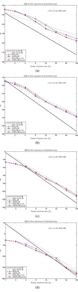
In Figs. 4 and 5 we plot the CRB (for ) or the lower and upper bounds of (25) when , as well as the MSE of the ML and AML estimators, as a function of , and compare the case where is known to the case where it is estimated from (67) with snapshots in the secondary data. The following observations can be made:
• there is almost no difference between the MLE and the AMLE, and therefore the latter should be favored since it does not require evaluating modified Bessel functions. • the MSE in the case where is known is lower than that
when is to be estimated, which is expected. However, the difference is smaller when : in other words, it seems that adaptive whitening is not so much penalizing with small while it seems more crucial for . In-deed, for small , what matters most is the fact that some snapshots are nearly noiseless, and this is more influential than obtaining a very good whitening.
• the decrease of the MSE for is roughly of the order . When , this rate is significantly increased and the MSE decreases very quickly as , as predicted by the analysis above. This rate of convergence is also ob-served in Fig. 6 where we consider a scenario with two sources at .
• the upper bound in (25) seems to provide quite a good approximation of the actual MSE, at least for large enough.
The influence of is investigated in Fig. 7, where one can observe that about is necessary for the performance with estimated to be very close to the performance for known . However, as indicated above, this is less pronounced when
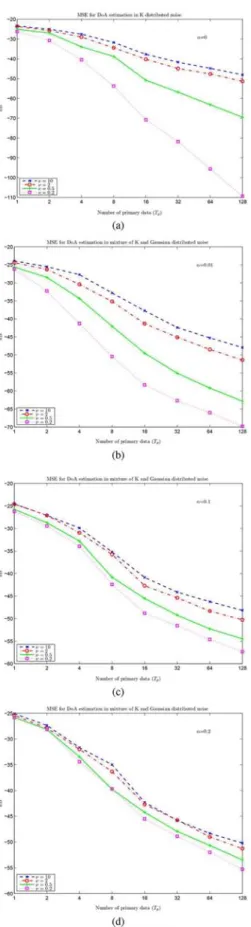
, where the difference becomes smaller with lower . Finally, we investigate whether the rate of convergence of the MLE or AMLE when varies is impacted by a small amount of Gaussian noise. More precisely, we run simulations where the data is generated as
(68) where , i.e., the noise is a mixture of -distributed noise and Gaussian distributed noise. The
covari-Fig. 7. Cramér-Rao bounds and mean square error of estimators versus . dB, and varying .
ance matrix of the noise is now
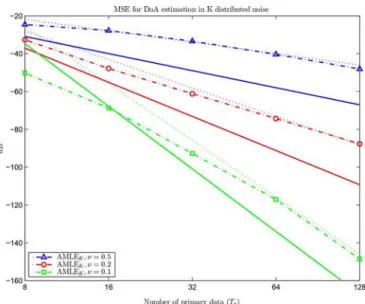
Fig. 8. Mean square error of AMLE versus in the case of a mixture of -distributed and Gaussian distributed noise. dB, and varying .
distribution with parameter and known covariance matrix . In Fig. 8, we display the MSE of the AML estimator versus and versus for different values of . Clearly, the rate of convergence of the estimator is affected by a small amount
of Gaussian noise, even when is small. This indicates that, if noise is not purely -distributed with small , we recover the usual behavior of the MSE versus .
V. CONCLUSION
In this paper we addressed the DoA estimation problem in -distributed noise using two data sets. The main result of the paper was to show that, when the shape parameter of the tex-ture Gamma distribution is below 1, the FIM is unbounded. On the other hand, for , the FIM is bounded and we derived an accurate closed-form approximation of the CRB. The max-imum likelihood estimator was derived as well as an approxi-mation, which induces non significant losses compared to the exact MLE. In the non regular case where , we derived lower and upper bounds on the mean-square error of the (A)ML estimates and we showed that the rate of convergence of these (A)ML estimates is about where is the number of snapshots.
REFERENCES
[1] H. L. Van Trees, Optimum Array Processing. New York, NY, USA: John Wiley, 2002.
[2] J. F. Böhme, “Estimation of spectral parameters of correlated signals in wavefields,” Signal Process., vol. 11, no. 4, pp. 329–337, 1986. [3] P. Stoica and A. Nehorai, “MUSIC, maximum likelihood and
Cramér-Rao bound,” IEEE Trans. Acoust., Speech, Signal Process., vol. 37, no. 5, pp. 720–741, May 1989.
[4] P. Stoica and A. Nehorai, “Performance study of conditional and unconditional direction of arrival estimation,” IEEE Trans. Acoust.,
Speech, Signal Process., vol. 38, no. 10, pp. 1793–1795, Oct. 1990.
[5] P. Stoica and A. Nehorai, “MUSIC, maximum likelihood and Cramér-Rao bound: Further results and comparisons,” IEEE Trans.
Acoust., Speech, Signal Process., vol. 38, no. 12, pp. 2140–2150, Dec.
1990.
[6] B. Friedlander and A. Weiss, “Direction finding using noise covariance modeling,” IEEE Trans. Signal Process., vol. 43, no. 7, pp. 1557–1567, July 1995.
[7] H. Ye and R. D. DeGroat, “Maximum likelihood DOA estimation and asymptotic Cramér-Rao bounds for additive unknown color noise,”
IEEE Trans. Signal Process., vol. 43, no. 4, pp. 938–949, Apr. 1992.
[8] V. Nagesha and S. M. Kay, “Maximum likelihood estimation for array processing in colored noise,” IEEE Trans. Signal Process., vol. 44, no. 2, pp. 169–180, Feb. 1996.
[9] M. Viberg, P. Stoica, and B. Ottersten, “Maximum likelihood array processing in spatially correlated noise fields using parameterized sig-nals,” IEEE Trans. Signal Process., vol. 45, no. 4, pp. 996–1004, Apr. 1997.
[10] B. Göransson and B. Ottersten, “Direction estimation in partially un-known noise fields,” IEEE Trans. Signal Process., vol. 47, no. 9, pp. 2375–2385, Sept. 1999.
[11] C. J. Coleman, “The directionality of atmospheric noise and its impact upon an HF receiving system,” in Proc. 8th Int. Conf. HF Radio Syst.
Tech., Guildford, U.K., 2000, pp. 363–366.
[12] Y. I. Abramovich, G. S. Antonio, and G. J. Frazer, “Over-the horizon radar signal-to-external noise ratio improvement in over-sampled uni-form 2D antenna arrays: Theoretical analysis of superdirective SNR gains,” in Proc. IEEE Radar Conf., Ottawa, Canada, Apr. 29–May 3, 2013, pp. 1–5.
[13] Y. I. Abramovich and G. S. Antonio, “Over-the horizon radar potential signal parameter estimation accuracy in harsh sensing environment,” in Proc. IEEE Int. Conf. Acoust., Speech, Signal Process., Florence, Italy, May 4–9, 2014, pp. 801–804.
[14] Y. I. Abramovich, N. K. Spencer, and P. Turcaj, “Two-set adaptive detection-estimation of Gaussian sources in Gaussian noise,” Signal
Process., vol. 84, no. 9, pp. 1537–1560, Sep. 2004.
[15] K. Werner and M. Jansson, “Optimal utilization of signal-free samples for array processing in unknown colored noise fields,” IEEE Trans.
Signal Process., vol. 54, no. 10, pp. 3861–3872, Oct. 2006.
[16] T. George, Handbook of Atmospherics. Boca Raton, FL, USA: CRC Press, 1982.
[17] Characteristics and Applications of Atmospheric Noise Data “Charac-teristics and applications of atmospheric noise data,”, ITU Rep. 322-3, 1983.
[18] “Radio noise,” International Communication Union Recommendation ITU-R P.372-11, Sep. 2013.
[19] E. Conte and M. Longo, “Characterisation of radar clutter as a spheri-cally invariant process,” Proc. Inst. Electr. Eng.—Radar, Sonar, Navig., vol. 134, no. 2, pp. 191–197, Apr. 1987.
[20] C. J. Baker, “Coherent K-distributed sea clutter,” in Proc. Inst. Electr.
Eng.—Radar, Sonar, Navig., Apr. 1991, vol. 138, no. 2, pp. 89–92.
[21] M. Rangaswamy, “Spherically invariant random processes for mod-eling non-Gaussian radar clutter,” in Proc. 27th Asilomar Conf., Pacific Grove, CA, USA, Nov. 1–3, 1993, pp. 1106–1110.
[22] J. B. Billingsley, A. Farina, F. Gini, M. V. Greco, and L. Verrazzani, “Statistical analyses of measured radar ground clutter data,” IEEE
Trans. Aerosp. Electron. Syst., vol. 35, no. 2, pp. 579–593, Apr. 1999.
[23] E. Conte, A. De Maio, and C. Galdi, “Statistical analysis of real clutter at different range resolutions,” IEEE Trans. Aerosp. Electron. Syst., vol. 40, no. 3, pp. 903–918, Jul. 2004.
[24] E. Conte, A. De Maio, and A. Farina, “Statistical tests for higher order analysis of radar clutter—Their analysis to L-band measured data,”
IEEE Trans. Aerosp. Electron. Syst., vol. 41, no. 1, pp. 205–218, Jan.
2005.
[25] T. W. Anderson and K.-T. Fang, “Theory and applications of ellipti-cally contoured and related distributions,” Tech. Rep. 24, Sep. 1990, Department of Statistics, Stanford University.
[26] K. T. Fang and Y. T. Zhang, Generalized Multivariate Analysis. Berlin, Germany: Springer-Verlag, 1990.
[27] E. Ollila, D. Tyler, V. Koivunen, and H. Poor, “Complex elliptically symmetric distributions: Survey, new results and applications,” IEEE
Trans. Signal Process., vol. 60, no. 11, pp. 5597–5625, Nov. 2012.
[28] K. J. Sangston, F. Gini, and M. S. Greco, “Coherent radar target detec-tion in heavy-tailed compound-Gaussian clutter,” IEEE Trans. Aerosp.
Electron. Syst., vol. 48, no. 1, pp. 64–77, Jan. 2012.
[29] F. Pascal, Y. Chitour, J.-P. Ovarlez, P. Forster, and P. Larzabal, “Covariance structure maximum-likelihood estimates in compound Gaussian noise: Existence and algorithm analysis,” IEEE Trans.
Signal Process., vol. 56, no. 1, pp. 34–48, Jan. 2008.
[30] O. Besson and Y. I. Abramovich, “On the Fisher information matrix for multivariate elliptically contoured distributions,” IEEE Signal Process.
Lett., vol. 20, no. 11, pp. 1130–1133, Nov. 2013.
[31] M. Greco and F. Gini, “Cramér-Rao lower bounds on covariance ma-trix estimation for complex elliptically symmetric distributions,” IEEE
Trans. Signal Process., vol. 61, no. 24, pp. 6401–6409, Dec. 2013.
[32] I. S. Gradshteyn and I. M. Ryzhik, Table of Integrals, Series and
Prod-ucts, ser. Alan Jeffrey Editor, 5th ed. New York, NY, USA: Aca-demic, 1994.
[33] N. El Korso, A. Renaux, and P. Forster, A. Coruña, Ed., “CRLB under -distributed observation with parameterized mean,” in Proc. 8th
IEEE Sensor Array Multichannel Signal Process. Workshop, Spain,
Jun. 22–25, 2014, pp. 461–464.
[34] A. Baricz and S. Ponnusamy, “On Turán type inequalities for modified Bessel functions,” in Proc. Amer. Math. Soc., Feb. 2013, vol. 141, no. 2, pp. 523–532.
[35] I. A. Ibragimov and R. Z. Has’minskii, Statistical Estimation
Asymp-totic Theory, ser. Application of Mathematics, A. V. Balakrishnan,
Ed. New York, NY, USA: Springer-Verlag, 1981, vol. 16.
[36] A. Renaux, P. Forster, E. Chaumette, and P. Larzabal, “On the high-SNR conditional maximum-likelihood estimator full statistical characterization,” IEEE Trans. Signal Process., vol. 54, no. 12, pp. 4840–4843, Dec. 2006.
[37] E. J. Gumbel, “Les valeurs extrêmes des distributions statistiques,”
An-nales de l’Institut Henri Poincaré, vol. 5, no. 2, pp. 115–158, 1935.
[38] B. Gnedenko, “Sur la distribution limite du terme maximum d’une série aléatoire,” Ann. Math. Statist., vol. 44, no. 3, pp. 423–453, Jul. 1943. [39] E. J. Gumbel, Statistics of Extremes. New York, NY, USA: Columbia
Univ. Press, 1958.
[40] D. E. Tyler, “A distribution-free M-estimator of multivariate scatter,”
Ann. Statist., vol. 15, no. 1, pp. 234–251, Mar. 1987.
[41] Y. Chitour and F. Pascal, “Exact maximum likelihood estimates for SIRV covariance matrix: Existence and algorithm analysis,” IEEE
Trans. Signal Process., vol. 56, no. 10, pp. 4563–4573, Oct. 2008.
[42] Y. I. Abramovich and N. K. Spencer, “Diagonally loaded normalised sample matrix inversion (LNSMI) for outlier-resistant adaptive fil-tering,” in Proc. ICASSP, Honolulu, HI, Apr. 2007, pp. 1105–1108. [43] Y. Chen, A. Wiesel, and A. O. Hero, “Robust shrinkage estimation of
high-dimensional covariance matrices,” IEEE Trans. Signal Process., vol. 59, no. 9, pp. 4097–4107, Sep. 2011.
[44] A. Wiesel, “Unified framework to regularized covariance estimation in scaled Gaussian models,” IEEE Trans. Signal Process., vol. 60, no. 1, pp. 29–38, Jan. 2012.
[45] F. Pascal, Y. Chitour, and Y. Quek, “Generalized robust shrinkage es-timator and its application to STAP detection problem,” IEEE Trans.
Signal Process., vol. 62, no. 21, pp. 5640–5651, Nov. 2014.
[46] Y. I. Abramovich and O. Besson, “Regularized covariance matrix estimation in complex elliptically symmetric distributions using the expected likelihood approach—Part 1: The oversampled case,” IEEE
Trans. Signal Process., vol. 61, no. 23, pp. 5807–5818, Dec. 2013.
[47] O. Besson and Y. I. Abramovich, “Regularized covariance matrix es-timation in complex elliptically symmetric distributions using the ex-pected likelihood approach—Part 2: The under-sampled case,” IEEE
Trans. Signal Process., vol. 61, no. 23, pp. 5819–5829, Dec. 2013.
Yuri I. Abramovich (M’96–SM’06–F’08) received
the Dipl.Eng. (Hons.) degree in radio electronics in 1967 and the Cand.Sci. degree (Ph.D. equivalent) in theoretical radio techniques in 1971, both from the Odessa Polytechnic University, Odessa (Ukraine), U.S.S.R., and in 1981, he received the D.Sc. degree in radar and navigation from the Leningrad Institute for Avionics, Leningrad (Russia), U.S.S.R.
From 1968 to 1994, he was with the Odessa State Polytechnic University, Odessa, Ukraine, as a Research Fellow, Professor, and ultimately as Vice-Chancellor of Science and Research. From 1994 to 2000, he was at the Cooperative Research Centre for Sensor Signal and Information Processing (CSSIP), Adelaide, Australia. From 2000 to 2010, he was with the Australian Defence Science and Technology Organisation (DSTO), Adelaide, as Principal Research Scientist, seconded to CSSIP until its closure in 2006. He is now with WR Systems in Fairfax, Virginia as a Principal Research Scientist. His research interests are in signal processing (particularly spatio-temporal adaptive pro-cessing, beamforming, signal detection and estimation), its application to radar (particularly over-the-horizon radar), electronic warfare, and communication. He is currently an Associate Editor of IEEE TRANSACTIONS ONAEROSPACE ANDELECTRONICSYSTEMSand previously served as Associate Editor of IEEE TRANSACTIONS ONSIGNALPROCESSINGfrom 2002 to 2005.
Olivier Besson (SM’04) received the Ph.D. degree
in signal processing from Institut National Polytech-nique Toulouse in 1992. He is currently a professor with the department of Electronics, Optronics and Signal of ISAE-Supaéro, Toulouse, France. His research interests are in statistical array processing, adaptive detection and estimation, with application to radar. Dr. Besson is a former member of the SAM technical committee of the IEEE Signal Processing Society.
Ben A. Johnson (S’04–M’09–SM’10) received a
Bachelor of Science (cum laude) degree in physics at Washington State University in 1984, a Master of Science degree in digital signal processing at University of Southern California in 1988, and a Ph.D. from the University of South Australia in 2009, focusing on application of spatio-temporal adaptive processing in HF radar. He is an LM Senior Fellow with Lockheed Martin IS&GS, as well as an adjunct research fellow at the University of South Australia.