Calibration and reliability of an alluvial aquifer model using inverse modelling and sensitivity analysis

Texte intégral

(1)Calibration and reliability of an alluvial aquifer model using inverse modelling and sensitivity analysis C. RENTIER1,2, S. BROUYERE1,2 & A. DASSARGUES2 1. National Fund for Scientific Research of Belgium Laboratoires de Géologie de l'Ingénieur, d'Hydrogéologie et de Prospection Géophysique (L.G.I.H.), University of Liège Bât. B19, B-4000 Liège, Belgium e-mail : crentier@lgih.ulg.ac.be 2. Abstract A three layer groundwater model was constructed in order to assess the discharge that is flowing through the alluvial aquifer of the Meuse River (Belgium) around the dam of Lixhe downwards from Liège. In a first approach, calibration was reached by trial-and-error. Then an inverse modelling technique, using PEST computer code, was used. Calibration was performed for two actual situations : (1) natural flow conditions and (2) pumping conditions. Results from the trial-and-error calibration and from the automatic calibration are compared. When many parameters are optimized by a calibration, such as in this case, different sets of data may produce identical results. A sensitivity analysis was performed to study the effect on the computed flow rate of a change in the parameter values such as hydraulic conductivity, recharge and conductance of the riverbed. The main objectives of such an analysis consist in determining (1) the influence of the various parameters within the aquifer on groundwater flow and heads; (2) the most sensitive parameter and (3) the reliability of the calibrated model.. INTRODUCTION The dam of Lixhe on the Meuse River, downwards from Liege (Belgium), currently exploited as a hydroelectric power station, splits the river in two reaches for which the water level difference is about 5 meters. This situation causes the groundwater flow to pass through the alluvial aquifer around the dam. This paper describes (1) the calibration of the groundwater model using a nonlinear-regression parameter estimation method to evaluate the flow rate that goes round the Lixhe’s dam and (2) the sensitivity analysis performed to quantify the reliability of the calibrated model.. CONCEPTUAL AND NUMERICAL GROUNDWATER FLOW MODEL The alluvial plain of the Meuse River is characterized by a fluvial sedimentation composed of coarse gravels at the base overlaid by gravels mixed in a sandy or silty matrix. A shale bedrock of Primary age can be considered as the impervious bottom of the alluvial aquifer except for its widely altered upper part. In order to assess the discharge that is flowing through the alluvial aquifer around Lixhe’s dam, a local three layer model was used with an upper continuous low permeability gravel unit (gravels mixed in a sandy-silty matrix), a permeable coarse gravel layer, and a bottom layer representing the altered shale unit. The 3D groundwater model was build using the GMS environment and the finitedifference MODFLOW code. The grid was 51 rows by 55 columns with cell lengths.

(2) ranging from 5 to 50 m and refined near the pumping well PRD. Where the Meuse River is fully canalized (upstream the dam) a no-flux boundary condition is chosen and constant head boundaries are chosen elsewhere (Fig. 1). On the North, East and South limits, constant head boundaries were set with values coming from extrapolation of the available head measurements. No argument can be found to justify an important piezometric variation between the three different geologic horizons, so it was decided to define the same boundary conditions for each of these layers. The Berwinne River confluence with the Meuse River is located downstream Lixhe’s dam, was simulated as a head-dependent-flow boundary.. 0m. Lixhe’s dam. 500 m. Berwinne River Pumping well PRD. Meuse River. N. Well River Constant Head. Fig. 1 Model grid and conceptual representation of the problem.. Theoretically, many parameters (referring here to any quantity being estimated) can be adjusted in order to calibrate the flow model : hydraulic conductivity, recharge, conductance coefficient of the river,... More than ever, the uniqueness of the model calibration cannot be addressed. So it was decided to set some parameters to specified values and to calibrate the model only by fitting hydraulic conductivity values of the second layer which constitutes the most permeable unit. Values of the fixed parameters were chosen based on isolated field measurements or expert opinion. Hydraulic conductivity of the first layer, which represents sandy and silty gravels, was fixed to 5.10-4 m s-1. As thickness and hydraulic conductivity of the weathered bedrock were not perfectly known, it was rather decided to work with transmissivity values. The transmissivity of this third layer was set to 10-6 m2 s-1. A uniform aquifer recharge of 200 mm year-1 was applied on top of the model. Conductance of a riverbed (CRIV) between the river and the aquifer corresponds to the hydraulic conductivity of the riverbed material (KRIV) multiplied by the length (L) and the width (W) of the river in.

(3) each cell and divided by the riverbed’s thickness (M) : CRIV = KRIV.L.W / M. The riverbed’s hydraulic conductivity was fixed to 10-7 m s-1.. PARAMETER ESTIMATION METHOD The PEST computer code, used in this study, is documented by Doherty (1994). It uses nonlinear regression to estimate parameters of groundwater flow systems. Nonlinear regression makes calibration more efficient and objective by adjusting parameters automatically, using the response of the model to changes in parameter values as a guide, until finding the values that minimize the maximum likelihood objective function φ (b) . In many circumstances, smaller values of the objective function indicate improved models. The maximum likelihood objective function is calculated as : n. φ (b) = ∑ ( wi ri ) 2. (1). i =1. where φ (b) is a np x 1 vector containing parameter values; np is the number of parameters estimated by regression; n is the number of observations (hydraulic heads for this model); wi is the weight assigned to the error in the observed value of measurement i and ri is the residual between observed and simulated values of measurement i . Weights are calculated according to procedures described by Doherty (1994) to account for measurement error in the observed values : they are inversely proportional to the standard deviation of the field or laboratory measurements to which they pertain :. wi = σ / σ i. (2). where σ is the common error standard deviation and σ i is the standard deviation of the measurement error of the i th observation (accuracy of the measurement). Parameter correlation coefficients measure the correlation between any pair of estimated parameter, that is coordinated linear changes in parameter values produce the same heads at observation locations (Poeter & Hill, 1997). These coefficients are calculated by :. ρij =. σ ij σ ii σ jj. (3). where σ ij are elements of the variance-covariance matrix C (b) for the final estimated parameters b . Correlation coefficient can range between [-1,+1]. Absolute values near 1 indicate that correlation exists between parameters. Smaller absolute values indicate less or no such correlation. When extreme correlation exists between parameters, the final estimates will depend strongly on the starting parameter values. Parameter estimates obtained through nonlinear regression are likely to be reliable if the estimates are precise and uncorrelated, and if the residuals are random and normally distributed..

(4) MODEL CALIBRATION. The model was calibrated on 12 piezometric head measurements for two actual situations : (1) natural flow conditions and (2) pumping conditions. In a first approach, calibration was reached by trial-and-error (Brouyère & Monjoie, 1998), adjustments were made manually until a reasonable match between calculated and observed heads was produced. In a second approach, an inverse modelling technique, using PEST, was used to find automatically the best match of calculated to observed heads by estimating the values of the non-fixed parameters. Both model calibrations are compared in figure 2. Some statistics as the residual mean (RM), the absolute residual mean (ARM), the residual standard deviation (RSD) and the objective function are calculated in table 1 for both natural flow and pumping conditions. Table 1 Statistics on model results for both trial-and-error and automatic calibration.. Trial-and-error calibration Natural conditions Pumping conditions Automatic calibration Natural conditions Pumping conditions. φ. (m2). RM (m). ARM (m). RSD (m). -0.003 0.031. 0.046 0.040. 0.071 0.162. 254 701. -0.001 0.039. -0.003 -0.045. 0.018 0.151. 17 352. The data to be matched are all of same type (heads) and were collected identically, so each of them was considered to have the same experimental error and therefore they were all assigned equal weights. Measurement errors were evaluated at 1 cm for every well except for the pumping well in the pumping condition where it was estimated at 5 cm. According to table 1 and figure 2, the results obtained by nonlinear regression obviously improve the calibration. All the K-values obtained by calibration for the second layer were reasonable and agreed with the measured values ; unreasonable optimized values would have indicated model error (Poeter & Hill, 1996), so their absence makes it more likely that the model accurately represents the groundwater system. In natural conditions, some of the correlation coefficient values were near unity, indicating that the corresponding estimated K-values were strongly correlated. Therefore we had to set one of these estimated K-zone to a specified value to remove the correlation. In pumping conditions, less correlation existed between estimated Kvalues, so estimation of the best fit parameters could be performed. In fact, flow observation (like pumping discharge) generally decreases the correlation between parameters that is present in cases where only head observations are available (Poeter & Hill, 1997) and so unique parameter estimates can be obtained. For the final calibration, the calculated discharge flowing through the alluvial aquifer around the dam of Lixhe in natural conditions was estimated at 624 m3 hour-1. Automatic calibration. Trial -and-error calibration 0.24. D5. 0.00 -0.12 -0.24. D7 D1 D1 1 D2 D1 0 D3 D6 PRD D8 D9. 0.12 0.00 -0.12 -0.24. D4 D5. D7 D1 D11 D3 PRD D1 0 D2 D8 D9 D6. Calculated heads (m). 0.12. (b) Residual error (m). (a). D4. Residual error (m). Natural condi tions. 0.24. 51. (e) 50 49 48.

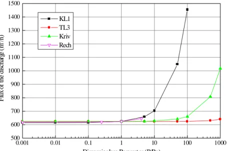
(5) Fig. 2 Graphical comparison between trial-and-error calibration and automatic calibration for natural and pumping conditions : (a),(b),(c),(d) observed heads versus residual error and (e),(f) observed versus calculated heads.. SENSITIVITY ANALYSIS. The inverse modelling technique was used to estimate the discharge groundwater flow around the Lixhe’s dam. Accuracy of the results depends on the reliability of the specified parameters (inferred from isolated measurements or expert opinion). The effect on the computed flow rate of a change in these fixed parameter values is studied by a deterministic sensitivity analysis. The main objectives of such an analysis are to determine (1) the influence of the various parameters within the aquifer system on groundwater flow estimation; (2) the most sensitive parameter and (3) the reliability of the calibrated model. The reference simulation corresponds to the case using the most likely values for the fixed parameters. The sensitivity simulations are deterministic in that only one parameter value is changed for each simulation, all other parameters are kept at the baseline values. Hydraulic conductivity of the first layer (KL1), equal in the reference case to 5.10-4 m s-1, was varied from 5.10-7 to 5.10-2 m s-1. From a reference value of 10-6 m2 s-1, the variation range of the third layer’s transmissivity (TL3) was 10-9 to 10-3 m2 s-1. Hydraulic conductivity of the riverbed KRIV (10-7 m2 s-1) was varied from 10-10 to 10-4 m2 s-1. Finally the recharge (Rech) of 200 mm year-1 ranged from 0 mm year-1 (supposing no infiltration and total surface runoff) to 800 mm year-1 (supposing total recharging infiltration, no evapotranspiration and no surface runoff). The corresponding fluxes are shown graphically in Figure 3. It can be observed (Fig. 3) that for each parameter there is a threshold (P/P0 = 1 for KL1 and Rech, P/P0 = 5 for KRIV and P/P0 = 100 for TL3) below which parameter value changes do not affect the order of magnitude of the discharge flux. In this case, the flux of discharge of the second layer (607 m3 hour-1) is quite smaller then the one calculated for the entire model (624 m3 hour-1). The constant head boundaries fixed on model limits impose a certain flux through the second layer that does not change much when the other parameters decrease. On the other hand, beyond the thresholds, the flow rate increases with the parameter values but differently depending on the.

(6) parameter. Discharge estimation is much more sensitive to KL1 and Rech than to KRIV or TL3, indicated by a larger change in discharge flux for a same ratio of change in parameter values. Sensitive but relatively certain parameters like Rech and uncertain but insensitive parameters such as TL3 do not produce significative changes in flow rate, so efforts to reduce model uncertainty should first focus on reducing the parameter uncertainty on KL1 and KRIV (more field measurements). 1500 1400. KL1 TL3 Kriv Rech. Flux of the discharge (m3/h). 1300 1200 1100 1000 900 800 700 600 500 0.001. 0.01. 0.1. 1. 10. 100. 1000. Dimensionless Parameter (P/Po). Fig. 3 Impact of errors in parameters over the estimated discharge.. CONCLUSION. In this study, a more reliable model calibration was reached by performing nonlinear regression instead of trial-and-error calibration. The sensitivity analysis showed that some uncertain parameters (KL1 and KRIV) have a significant impact on the results and should be carefully determined: further model refinements should be accomplished by integration of new data on these sensitive and uncertain parameter values, rather than trying to reduce uncertainty about less important parameters such as TL3 or Rech.. REFERENCES Brouyère, S. & Monjoie, A. (1998) Barrage de Lixhe : étude et modélisation des débits de contournement du barrage par la plaine alluviale en rive droite de la Meuse. LGIH Rapport SPE/981, 23 p (unpublished). Doherty, J. (1994) PEST. Watermark Computing, Corinda, Australia, 122 p. Poeter, E. P. & Hill, M. C. (1996) Unrealistic parameter estimates in inverse modelling : a problem or a benefit for model calibration? In : ModelCARE’96 : Calibration and Reliability in Groundwater Modelling (ed. by K. Kovar & P. van der Heijde) (Proc. Golden, Colorado, September 1996), 277-285. IAHS Publ. No. 237. Poeter, E. P. & Hill, M. C. (1997) Inverse models : a necessary next step in groundwater modelling. Ground Water 35(2), 41-52..

(7)