Mathematical methods for implicit solvation models in quantum chemistry

HAL Id: tel-01919793

https://tel.archives-ouvertes.fr/tel-01919793

HAL is a multi-disciplinary open access archive for the deposit and dissemination of sci-entific research documents, whether they are pub-lished or not. The documents may come from teaching and research institutions in France or abroad, or from public or private research centers.

L’archive ouverte pluridisciplinaire HAL, est destinée au dépôt et à la diffusion de documents scientifiques de niveau recherche, publiés ou non, émanant des établissements d’enseignement et de recherche français ou étrangers, des laboratoires publics ou privés.

Mathematical methods for implicit solvation models in

quantum chemistry

Chaoyu Quan

To cite this version:

Chaoyu Quan. Mathematical methods for implicit solvation models in quantum chemistry. Mathemat-ical Physics [math-ph]. Université Pierre et Marie Curie - Paris VI; Rheinisch-westfälische technische Hochschule (Aix-la-Chapelle, Allemagne), 2017. English. �NNT : 2017PA066587�. �tel-01919793�

Thèse de Doctorat de

l’Université Pierre et Marie Curie

Présentée et soutenue publiquement le 21 Novembre 2017 pour l’obtention du grade de

Docteur de l’Université Pierre et Marie Curie

Spécialité : Mathématiques Appliquées par

Chaoyu QUAN

sous la direction de

Yvon MADAY et Benjamin STAMM

Mathematical Methods for Implicit Solvation Models

in Quantum Chemistry

après avis des rapporteurs

M. Martin J. GANDER & M. Aihui ZHOU

devant le jury composé de

M. Eric CANCES Examinateur M. Pascal FREY Examinateur M. Martin J. GANDER Rapporteur Mme. Laura GRIGORI Examinateur M. Yvon MADAY Directeur de thèse M. Jean-Philip PIQUEMAL Examinateur M. Benjamin STAMM Directeur de thèse M. Aihui ZHOU Rapporteur

École Doctorale de Sciences Mathématiques Faculté de Mathématiques

Chaoyu QUAN :

Sorbonne Universités, UPMC Univ Paris 06, UMR 7598, Laboratoire Jacques-Louis Lions, F-75005, Paris, France.

First and foremost I would like to thank my advisors Yvon Maday and Benjamin Stamm. It has been a great honor to be their Ph.D. student. The first time that I met Yvon was in his course on the variational discretization of the elliptic partial differential equations, which was attractive and inspired me to start my researches with him. Obviously, this is one of the best decisions that I have ever made in my life. Yvon is very kind, experienced in academic researches, full of new ideas and good at seeking funding etc. To me, he himself is the best model of what a good researcher should be, which is important to encourage a beginner in the academic world like me. Benjamin is both an advisor and a friend to me. As the advisor, he has taught me many things associated with researches, such as how to think over questions in a strict way, how to use Matlab efficiently, how to write a professional article etc. As a friend, he cares about my life in Paris, including the visa, the housing, the food etc. I feel really happy to be his first Ph.D. student and appreciate all his contributions of time, ideas and patience to me.

Then, I want to thank Pascal Frey and Eric Cancès for their fruitful discussions with us on the molecular surfaces and the implicit solvation models. Pascal has pro-vided me with some good advices on meshing the molecular surfaces. Furthermore, I do appreciate his efforts on the funding of my postdoc in the CalSimLab, Univer-sité Pierre et Marie Curie. Eric has discussed with us about the implicit solvation models. In fact, the second part of my thesis is based on his work on the integral equation formulation of the polarizable continuum models and on the domain “spher-ical” decomposition method for the conductor-like screening models. Moreover, I would thank Eric for the recommendation letter for my postdoc applications.

In regards to the academic discussions, I also thank Filippo Lipparini, Louis

4

gardére, Benedetta Mennucci and Jean-Philip Piquemal. They have helped me to know more about the quantum chemistry.

Besides, I want to thank the two reviewers of my thesis for their positive opinions. In particular, thank Martin J. Gander for changing his schedule in order to join my defense in Paris. Thank Aihui Zhou for taking a long journey from Beijing to Paris and for spending much time on the visa.

In my lab, Laboratoire Jacques-Louis Lions, there are many persons that I would like to thank for their help as well as their accompany, including Carlo Marcati, Geneviève Dusson, Étienne Polack, Amaury Hayat, Rim El Dbaissy, Gabriela Lopez Ruiz, Philippe Ung, Florian Omnes, Shuyang Xiang, Long Hu, Jiamin Zhu, Yashan Xu, Can Zhang, Haisen Zhang, Chen-Yu Chiang, Helin Gong, Yangyang Cao, Shijie Dong, Hongjun Ji, Yuqing Wu etc. In addition, I want to thank my good friends Wen Sun, Xianglong Duan, Qilong Weng, Bingxiao Liu and Zicheng Qian who do mathematical researches in Paris and come from the same Chinese university as me, University of Science and Technology of China. We have spent a pleasant time together in Paris.

Finally, I would like to thank my wife and my parents who always support me to do researches, and I also want to express my best wishes to my upcoming baby who motivates me to work hard.

Introduction 9

1 The larger context . . . 9

2 Implicit solvation models . . . 11

3 Domain decomposition methods for implicit solvation models . . . 20

I

Molecular Surfaces

31

1.2 Introduction to implicit surfaces . . . 36

1.3 Implicit molecular surfaces . . . 37

1.4 Solvent accessible surface . . . 39

1.5 Solvent excluded surface . . . 50

1.6 Construction of molecular surfaces . . . 59

1.7 Numerical results . . . 63

1.8 Conclusion . . . 67

2 Meshing molecular surfaces based on analytical implicit representa-tion 69 2.1 Introduction . . . 70

6 Contents

2.2 Molecular surfaces . . . 72

2.3 Construction of molecular surfaces . . . 77

2.4 Molecular inner holes . . . 80

2.5 Meshing . . . 82

2.6 Conclusion . . . 92

II

Domain Decomposition Method for Implicit Solvation

Models

95

3.2 Solute-solvent boundary . . . 103

3.3 Dielectric permittivity function . . . 105

3.4 Problem formulation and global strategy . . . 107

3.5 Domain decomposition strategy . . . 111

3.6 Single-domain solvers . . . 112

3.7 Numerical results . . . 119

3.8 Conclusion . . . 130

4 Domain Decomposition Method for the Poisson-Boltzmann Solva-tion Model 131 4.1 Introduction . . . 132 4.2 PB solvation model . . . 137 4.3 Problem transformation . . . 139 4.4 Strategy . . . 142 4.5 Single-domain solvers . . . 145

4.6 Global linear system . . . 148

4.7 Numerical results . . . 154

4.8 Conclusion . . . 158

Appendices 160

A Proof of Theorem 1.5.1 161

B Advancing-front algorithm for a spherical patch 165

C Appendices in Chapter 3 167 C.1 Well-posedness of (3.6.7) . . . 167 C.2 Computation of _∂θ∂Y_ℓm and _∂φ∂ Y_ℓm . . . 169 C.3 Computation of f (x) in (3.6.6) . . . 170 D Computation of C1, C2, F0 173 Bibliography 186

1

The larger context

Quantum chemistry aims at understanding the properties (such as spectroscopic observables, equilibrium geometry of the ground state or reactivity) of matter through the modeling of its behavior at a molecular scale [23, 24], where matter is described as an assembly of nuclei and electrons. This problem is known as the many-body prob-lem and its solution, the wave function Ψ, is described by the Schrödinger equation in its time-dependent

i_∂t∂Ψ(t) = HΨ(t), (1.1) or time-independent form

HΨ = EΨ, (1.2)

where H denotes the Hamiltonian of the molecular system under consideration and the constant E is the energy of the stationary state Ψ. The above two equations are very high dimensional differential equations whose solution can not even be ap-proximated for a small molecule directly. To make the problem more tractable, the nuclei structure computation and the electronic structure computation are usually considered separately, as the mass of a nuclei is several magnitudes heavier than the one of an electron (known as the Born-Oppenheimer approximation).

In fact, most physical and chemical phenomena of interest in chemistry and biol-ogy take place in the liquid phase, and it is relevant and crucial to model the solvent in these processes. The typical situation is that a solute (biological protein for exam-ple) is surrounded by the solvent. To describe the solvent effects on the solute, two approaches are commonly-used. The first one is to use an explicit solvation model, in which the simulated chemical system is composed of the solute molecule and a large number of explicit solvent molecules. The second one is to use an implicit solvation model (or continuum solvation model), in which the solute molecule is embedded in a cavity surrounded by a continuous medium representing the solvent, i.e., the average response of the solvent molecules over the phase-space of the solvent molecules in the sense of statistical mechanics. Comparing to the explicit solvation model, the com-putation of implicit solvation model is usually much less expensive in comcom-putational time, see [21, 109, 82] for an overview of the implicit solvation model.

10 1. The larger context

In the implicit solvation model, the solvent is usually treated as a polarizable continuum with a specific dielectric permittivity. Embedding the solute molecule in the continuous solvent, the solute’s charge distribution interacts with the continuous dielectric field and polarizes the surrounding medium, which in turn causes a change in the polarization on the solute. This defines the reaction potential, a response to the presence of the continuous environment. In quantum chemistry, where charge distributions come from ab initio methods, such as the Hartree-Fock (HF) electronic functionals or the Density Functional Theory (DFT), the implicit solvent models represent the solvent as a perturbation to the solute Hamiltonian in the following way [83, 109]:

H = HM_+HMS_{, (1.3)}

where HM _{is the Hamiltonian of the solute molecule M and H}MS _{is the interaction}

between the solute M and the solvent S.

Actually, HMS _{is a sum of different interaction operators, each of which is related}

to an interaction with a different physical origin. In the standard implicit solvation model, four interaction operators are usually used to describe the solute-solvent in-teraction [84, 83]. This gives thus four contribution terms to the solvation energy. Supplemented by a fifth describing contribution due to thermal motions of the molec-ular framework, the solvation energy G of M is written in the following form

G = Gcav+ Gel+ Gdis+ Grep+ Gtm, (1.4)

where the five terms on the right side represent respectively the cavitation, the elec-trostatic contribution, the dispersion, the repulsion and the thermal motion [83].

One main topic of this thesis is the computation of the electrostatic contribution

Gel, a crucial issue in the calculation of solvation free energy, which involves solving

a partial differential equation (PDE). To be precise, the electrostatic potential ψ of an implicit solvation model is characterized as follows

−∇ · ε(x)∇ψ(x) = 4πρ(x), in R3_{, (1.5)}

where ψ(x) ∼ _|x|1 as |x| → ∞. Here, ε(x) represents the space-dependent dielectric constant and ρ(x) represents the charge distribution of the solvation system. The electrostatic contribution Gel to the solvation energy, also denoted by Es in this

thesis, is given by Gel = Es= 1 2 ∫ R3ρ(x) (ψ(x)− ψ0(x)) dx, (1.6) where ψ0(x) = ∫ R3 ρ(x′) |x − x′_|dx′ (1.7)

For the sake of simplicity, it is usually assumed that the solute’s charge distribution function ρM(part of the whole charge distribution ρ) is supported in the solute cavity

Ω and is presented by the sum of M point charges in the form of

ρM(x) =

M

∑

i=1

qiδ(x− xi), (1.8)

where M is the number of solute atoms, qi represents the charge carried on the ith

atom with center xi, δ is the Dirac delta function. As a consequence, when the solvent

does not contain any ion, we have ρ = ρM and therefore, ψ0 can be derived easily.

In this thesis, we will develop two Schwarz domain decomposition methods for solving the PDEs of the form (1.5) for two implicit solvation models. But before that, we first see some of our achievements on the characterization of the solute-solvent interface, especially the so-called “smooth” molecular surface (or the solvent excluded surface). The solute-solvent interface, which determines both the solute cavity and the solvent region, plays a fundamental role in an implicit solvation model.

For the sake of completeness, the following part of introduction might be repeated latter in Chapter 1–4. If the reader wants to get a general idea of this thesis as well as its contribution, it is helpful to read this introduction. If the reader is only interested in a particular part, each chapter can be read directly.

2

Implicit solvation models

In this section, we focus on introducing some basic notations of implicit solva-tion models. We first introduce the solute cavity determined by the solute-solvent boundary, which is a fundamental concept of an implicit solvation model. Then, we introduce different kinds of implicit solvation models, classified by different physical laws describing the solute-solvent interaction. Briefly speaking, an implicit solvation model consists of a suitable solute cavity and a specific physical law.

2.1

Solute-solvent boundary: solute cavities

In an implicit solvation model, the solute molecule is embedded in a cavity (the solute cavity), denoted by Ω, surrounded by a continuous medium representing the solvent on a macroscopic scale. The definition of the solute cavity is not an in-trinsic property of the solute molecule. As a consequence, determining a suitable solute-solvent boundary is important. It builds an interface between the solute and the solvent respectively between the atomistic and the continuum description of the physical model. Physically speaking, the solute cavity, i.e., the region enclosed by the solute-solvent boundary, occupies the space of the solute molecule where the

sol-12 2. Implicit solvation models

Figure 1: Schematic diagram of the VdW-surface (green), the SAS (blue) and the SES (red).

vent molecules have no access. Therefore, a precise understanding and modeling of the nature of the solute-solvent boundary is essential. In fact, there are several well-established molecular surfaces that are usually chosen as the solute-solvent boundary: the van der Waals (VdW) surface, the Solvent Accessible Surface (SAS) and the Sol-vent Excluded Surface (SES).

2.1.1 Molecular surfaces

In the simplest model, atoms of a molecule are represented by VdW-balls with VdW-radii which are experimentally fitted, given the underlying chemical element, for example, the UFF radii [97]. As a consequence, the VdW-surface is defined as the topological boundary of the union of all VdW-balls.

In addition, the SAS and the SES were first introduced by Lee & Richards in the 1970s [67, 99], where the solvent molecules surrounding a solute molecule are reduced to spherical probes [109]. The SAS of a solute molecule is defined by rolling the center of an idealized spherical probe over the solute molecule, that is, the surface enclosing the region in which the center of a spherical probe can not enter. The SES is also called “the smooth molecular surface” or “the Connolly surface”, due to Connolly’s fundamental work [30]. It is defined by the same spherical probe rolling over the molecule, but now one considers the surface enclosing the region in which a spherical probe can not access. In other words, the SES is the boundary of the union of all possible probes that do not intersect the VdW-balls of the solute molecule, see Figure 1 for a 2D schematic diagram of different molecular surfaces. Indeed, the SES can be considered to be the prototype for the computational study of molecular surfaces.

The definition of VdW-surface is based on the model that each atom has a specific radius around the atom center. However, the definition of the VdW-surface has ignored the size and shape of the surrounding solvent molecules in solvation models. The definition of SAS has taken this into account by modeling them by idealized

Figure 2: 3D schematic of the SES illustrating the convex spherical patches (red), the toroidal patches (yellow) and the concave spherical patches (blue).

spherical probes with a certain probe radius. The definition of the SES is different from the SAS in the sense that not the probe center traces out the desired surface, but the surface of the probe. In the application of docking [76], the SES will not lead to the overlapping of neighboring surfaces since the SES does not inflate the atom radii but the SAS will.

Sometimes, the SAS can be non-connected: it can be composed of several separate surfaces. We call the outmost surface as the exterior Solvent Accessible Surface (eSAS) and the union of all separated surfaces as the complete Solvent Accessible Surface (cSAS), see Chapter 1 for details. Correspondingly, we will also propose the concept of the complete Solvent Excluded Surface (cSES) and the exterior Solvent Excluded Surface (eSES).

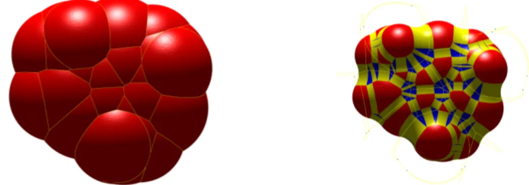
Both the VdW-surface and the SAS are composed of three parts: open spher-ical patches, open circular arcs (or circles) and intersection points (formed by the intersection of three or more spheres). Their geometric features are therefore easier to understand. The SES can be divided into three corresponding types of patches as presented in Connolly’s work [30]: convex spherical patches, toroidal patches and concave spherical patches, see Figure 2 for an illustration. Any point on a convex spherical patch of the SES has a closest point to the SAS on a spherical patch. Sim-ilarly, any point on a toroidal patch of the SES has a closest point to the SAS on a circular arc, and any point on a concave patch has a closest point to the SAS which is an intersection point.

Despite that the whole SES is smooth almost everywhere, self-intersections among different SES-patches can occur and often cause SES-singularities. This singularity problem has led to difficulty in associated researches on the SES, for example, the failure of SES meshing algorithms and the imprecise calculation of molecular areas or volumes, or has been circumvented by approximate techniques [28]. In 1996, Sanner treated some special cases of SES-singularity in his MSMS (Michel Sanner’s Molecular Surface) package for the analytical calculation of molecular areas and volumes, and the triangulation of molecular surfaces [102]. Nevertheless, to our knowledge, the complete characterization of the SES-singularities remains unsolved despite of a large

14 2. Implicit solvation models

number of contributions in literature [30, 102, 73, 52].

In this thesis, we will present a computable method to represent implicitly the molecular surfaces. We suppose that the solute molecule is composed of M atoms and the jth atom has a center cj and a VdW radius rj. The solvent probe radius is

denoted by rp. Thus, we can denote by fsas the signed distance function to the SAS

(negative inside the SAS and positive outside the SAS) as follows

fsas(p) = {

−∥p − xp

sas∥ if p lies inside the SAS,

∥p − xp

sas∥ if p lies outside the SAS,

(2.1)

where xp

sas denotes a closest point on the SAS to p. Note that there might exist more

than one closest point on the SAS and in this case xp

sas is chosen as one of them. The

implicit functions of the SAS (denoted by Γsas) and the SES (denoted by Γses) are

consequently deduced as follows

Γsas = fsas−1(0) and Γses = fsas−1(−rp),

which characterize mathematically these two molecular surfaces. However, the chal-lenge is that xp

sas is not easy to compute because the shape of the molecule can be as

complicated as possible.

In Chapter 1 of Part I, an efficient method for computing analytically the func-tion value of fsas will be proposed, which therefore gives a complete characterization

of the SES. In fact, it is based on three equivalence statements, which induces a nonoverlapping partition of R3_{. In addition, we redefine different types of}

SES-patches mathematically so that the SES-singularities will be characterized explicitly and no self-interaction will occur. By applying the Gauss-Bonnet theorem [35] and the Gauss-Green theorem [38], we will give an explicit formula of calculating analyti-cally all the molecular areas and volumes, in particular for the SES. These quantities are useful in many protein models, such as describing the hydration effects [100, 19]. Furthermore, the complete characterization of different molecular surfaces will allow us to visualize them more precisely.

2.1.2 Molecular visualization

Molecular visualization is helpful for researchers to understand the geometrical structure of a molecule and to illustrate charge distributions on molecular surfaces. This topic is of course intrinsically linked to the notion of a solute cavity.

Since the VdW surface and the SAS are topologically simple, it is more challenging to visualize the SES (the so-called “smooth” molecular surface). As mentioned in the above section, Sanner proposed the reduced surfaces and then the MSMS algorithm [102] for computing an (in fact approximately) analytical representation of the SES. In addition, this algorithm also provides a triangulation of the SES with a

user-Figure 3: The SES of three balls having the self-intersection problem (left, triangu-lation provided by the MSMS-algorithm) and the realistic SES (right, triangutriangu-lation provided by our algorithm).

specified density of vertices and therefore the molecular visualization based on this triangulation is feasible. Despite of the self-intersection problem among different SES-patches (see Figure 3 for an example where self-intersection occurs), the MSMS is still one of the most widely-used packages for molecular visualization. Besides, there are many other contributions on the molecular visualization [64, 89, 59], the visualization of molecular dynamics [55, 61], the Eulerian representation of SESs [73], the high-quality mesh generation of molecular surfaces [65] and so on.

Benefitting from the complete characterization of the SES for the first time (see Chapter 1), we are now able to develop a piecewise meshing algorithm for molecular surfaces which avoids the self-intersection between SES-patches. In Chapter 2 of Part I, we will first give a detailed strategy for constructing the data structures of molecu-lar surfaces, thanks to this analytical characterization. Then, a meshing algorithm for molecular surfaces, especially the SES, is developed, combining an advancing-front algorithm with the pre-computed data structures. The explicit characterization of all singularities resolves the issue of self-intersection that is experienced due to singu-larities as they can be computed prior to the meshing of the surface. This, in turn, allows the possibilities of meshing the SES exactly, in the sense that each vertex of the mesh lies exactly on the surface. Here, we emphasize that this is only possible due to the above-developed analysis of the molecular surfaces and it is not the case for the existing meshing algorithms. In addition, we propose an algorithm for filling molecular inner holes with virtual atoms for the reason that the appearance of these inner holes is not always justified in the solute cavity of the implicit solvation models, as this would mean that the solvent is present in these inner holes.

So far, we have introduced our achievements on the solute-solvent interface, in-cluding the complete characterization of molecular surfaces and the molecular visual-ization. Next, we will introduce different physical laws that describe the electrostatic potential of the implicit solvation model in different ways.

16 2. Implicit solvation models

2.2

Solute-solvent interaction: physical laws

Based on a suitable choice of solute-solvent boundary (interface), the implicit sol-vation model divides the whole space into the solute cavity and the solvent region. Further, the solvent is characterized in terms of its macroscopic physical properties, such as the dielectric permittivity and the ionic strength. Different types of implicit solvation model are consequently constructed as follows, based on different physical laws to model the electrostatic potential of the solute-solvent interaction: the Polar-izable Continuum Model (PCM), the COnductor-like Screen MOdel (COSMO) and the Poisson-Boltzmann (PB) solvation model.

2.2.1 Polarizable continuum model

The polarizable continuum model (PCM) [26, 109] is a widely-used type of implicit solvation model in computational chemistry to model solvation effects, in which the solvent is represented by a polarizable continuum. This implies that there is no charge in the solvent region and the charge distribution of the solvation system is the solute charge distribution ρM supported in the solute cavity. In the classical PCM with a

solute cavity Ω, the space-dependent dielectric permittivity ε(x) is defined as (see the right of Figure 4)

ε(x) =

{

1 x∈ Ω,

εs x∈ Ωc :=R3\Ω,

(2.2)

where εs is the (bulk) solvent dielectric constant and ε(x) has a jump on the

solute-solvent boundary Γ := ∂Ω.

With the above dielectric permittivity (2.2), the PDE (1.5) of the electrostatic potential ψ can be rewritten as

             −∆ψ = 4πρM, in Ω, −∆ψ = 0, in Ωc, [ψ] = 0, on Γ, [∂n(εψ)] = 0, on Γ, (2.3)

where n denotes the unit normal vector pointing outwards with respect to Ω, [ψ] and [∂n(εψ)] respectively denote the jump (inside Ω minus outside) of ψ and the jump of

the normal derivative of εψ on Γ. An integral equation formalism (IEF) [22, 81, 26] of this equation was proposed by E. Cancès, B. Mennucci and J. Tomasi, which has been the default PCM formulation in Gaussian [44]. This formalism transforms the original problem defined in the 3D space equivalently to an integral equation on the dielectric boundary and therefore the computational cost can be greatly reduced.

Figure 4: 2D schematic diagrams of the classical PCM (left) and the COSMO (right).

2.2.2 Conductor-like screening model

A reduced version of PCM is also popular in quantum chemistry, that is, the COnductor-like Screen MOdel (COSMO) [109], in which the solvent continuum is assumed to be conductor-like (see the right of Figure 4), i.e., one takes εs =∞ in Eq.

(2.2). That means that the dielectric permittivity function ε(x) is taken as

ε(x) =

{

1 x∈ Ω,

∞ x ∈ Ωc

. (2.4)

This reduced model is usually employed to approximate the PCM when the solvent dielectric permittivity εs is relatively large, for example, the (relative) dielectric

per-mittivity of water is εs= 78.4 at room temperature (25◦C).

In this case, the original PDE (1.5) of the electrostatic potential is simply a Pois-son equation defined on a bounded domain with a homogeneous Dirichlet boundary

condition _{

−∆ψ(x) = 4πρM(x), in Ω,

ψ(x) = 0, on Γ. (2.5)

Here, the electrostatic potential ψ vanishes on the solute-solvent boundary Γ because the solvent is idealized as perfect conductor and consequently there is no electric field in the solvent region.

Comparing to the PCM defined in R3_{, the COSMO is only a problem defined}

on the bounded domain Ω, which is consequently easier. As assumed, the charge distribution ρM of the solute molecule is already known. For calculating the

sol-vent effects with a finite dielectric constant εs, the electrostatic contribution to the

solvation energy Es _{is usually approximated by}

18 2. Implicit solvation models

where Es

∞is the electrostatic contribution to the solvation energy computed from the

COSMO by solving the PDE (2.5) and the factor f (εs) is empirically given by

f (εs) =

εs− 1

εs+ x

,

with x usually set to 0.5 based on theoretical arguments.

2.2.3 PB solvation model

The properties of numerous charged bio-molecules and their complexes with other molecules are dependent on not only the polarizable effects of the environment, but also on the ionic effects. In this case, the Poisson-Boltzmann (PB) solvation model [116, 86] takes into account both the solvent dielectric permittivity and the ionic strength, which is now widely-used. In such a model, the solvent is seen as a polar-izable continuum containing ions. The solvent dielectric permittivity is defined by (2.2) in the PCM and the movement of ions in solution is accounted for by Boltz-mann statistics. That is to say, the BoltzBoltz-mann equation is used to calculate the local density ci of the i-th type of ion as follows

ci = c∞i e

−Wi

kBT_{, (2.6)}

where c∞_i is the bulk ion concentration at an infinite distance from the solute molecule,

Wi is the work required to move the ion to the position from an infinitely far distance,

kB is the Boltzmann constant, T is the temperature in Kelvins (K). Combining (1.5),

(1.8) and (2.6), we derive the Poisson-Boltzmann equation as follows (see [40])

−∇ · [ε(x)∇ψ(x)] = 4πρM(x) + ∑ i ziec∞i e −zieψ(x) kBT _χΩc(x), (2.7)

where zie is the charge of the i-th type of ion, e is the elementary charge and χΩc is the characteristic function of the solvent region Ωc_.

In the PB solvation model with 1 : 1 electrolyte, there are two types of ions respectively with charge +e and −e (see Figure 5). With the assumption that ψ satisfies the low potential condition, i.e.,  eψ

kBT

 ≪ 1, the above Poisson-Boltzmann

equation can be linearized to (see [86] for this form)

−∇ · [ε(x)∇ψ(x)] + ¯κ(x)2

ψ(x) = 4πρM(x), (2.8)

which ψ is determined by the spatial dielectric permittivity function ε(x), the modi-fied Debye-Hückel parameter ¯κ(x) and the solute’s charge distribution function ρM(x).

Figure 5: 2D schematic diagrams of the Poisson-Boltzmann solvation model.

Poisson-Boltzmann equation can still be linearized to the same form (2.8).

The dielectric permittivity function is defined in the classical way

ε(x) =

{

1 x∈ Ω,

εs x∈ Ωc,

(2.9)

where εs is the solvent dielectric constant as previous. The modified Debye-Hückel

parameter is taken as ¯ κ(x) = { 0 in Ω, √ εsκ in Ωc, (2.10)

where κ is the Debye-Hückel screening constant representing the attenuation of in-teractions due to the presence of ions in the solvent region, which is related to the ionic strength I of the aqueous salt solution according to

κ2 = 8πe

2_N AI

1000εskBT

, (2.11)

where NA is the Avogadro constant.

In summary, we have presented in this part three types of physical law for the implicit solvation model, in three different cases of solvent: the polarizable continuum (PCM), the conductor-like continuum (COSMO) and the polarizable continuum con-taining ions (PB solvation model). In the following part, we introduce a particular kind of domain decomposition method for solving the electrostatic problem of these implicit solvation models.

20 3. Domain decomposition methods for implicit solvation models

3

Domain decomposition methods for implicit

sol-vation models

Implicit solvation models are widely-used in the chemistry community, but little interaction with applied mathematics can be observed despite the fact that solutions to partial differential equations need to be approximated. The underlying physical law is provided by electrostatic interaction involving elliptic operators.

In this section, we first introduce two state-of-art Schwarz domain decomposition (dd) methods respectively for solving the COSMO and the PCM: the ddCOSMO and the ddPCM. Then, we introduce two new Schwarz domain decomposition methods respectively for solving an SES-based PCM and the PB solvation model, which are contributions of this thesis. The methods generally consist of two steps:

[1] if the electrostatic problem is defined on an unbounded domain, transform the original problem equivalently to problems that are defined on a bounded domain and might be coupled by a non-local condition;

[2] develop a classical Schwarz domain decomposition method that decomposes the bounded domain into balls and only solve local coupled sub-problems restricted to balls.

For the SES-based PCM, we will first construct the model and then propose the corresponding domain decomposition method for solving it, called the ddPCM-SES method. Further, for the PB solvation model which is already established in Section 2.2.3, we will propose a domain decomposition method for solving it, which is called the ddLPB method.

3.1

ddCOSMO

To solve the electrostatic problem of the COSMO, the finite element method or the finite difference method can be used. However, the computational cost is too expensive for a large realistic molecule. In particular, meshing the solute cavity Ω of a complicated molecule is already too costly. The state-of-art COSMO solver is the ddCOSMO [25, 72, 69], a Schwarz domain decomposition method [96, 107] developed for solving the COSMO in the past several years, which has attracted much attention due to its impressive efficiency, that is, it performs about two orders of magnitude faster than other equivalent methods [69].

The crucial part consists in decomposing the domain into a union of balls and solving only each sub-problem restricted to a ball. Let Ω be the VdW-cavity or the

SAS-cavity, meaning that Ω is a union of overlapping balls in the following form Ω = M ∪ j=1 Ωj, Ωj = Brj(xj), (3.1)

where each Ωj denotes the j-th atomic VdW-ball (or SAS-ball) with center xj and

radius rj.

We then homogenize the COSMO equation (2.5) by defining

ψ0 = M ∑ i=1 qi |x − xi| , (3.2)

which satisfies−∆ψ0 = 4πρM(x) in R3. Here, ρMis given by Eq. (1.8). The reaction

potential ψr := ψ− ψ0 satisfies consequently the following Laplace equation with the

Dirichlet boundary condition

{

−∆ψr = 0, in Ω,

ψr =−ψ0, on Γ.

(3.3)

The reaction potential is indeed the electrostatic potential that is additionally created by the pressure of the solvent with respect to vacuum.

Using the Schwarz decomposition of Ω, this Laplace equation can be recast as the following group of coupled sub-equations, each restricted to Ωj:

{ −∆ψr|Ωj = 0 in Ωj, ψr|Γj = ϕr,j on Γj, (3.4) where Γj = ∂Ωj and ϕr,j = { ψ_r on Γi_j, − ψ0 on Γej. (3.5) Here, Γe

j is the external part of Γj not contained in any other ball Ωi (i ̸= j), i.e.,

Γe

j = Γ∩ Γj; Γij is the internal part of Γj, i.e., Γij = Ω∩ Γj (see Figure 6 for the

illustration of notations). In addition, ψ_r is defined as

ψ_r(x) = 1 |N (j, x)| ∑ i∈N (j,x) ψr|Ωi(x), ∀x ∈ Γ i j, (3.6)

where N (j, x) represents the index set of all balls such that x ∈ Ωi. In fact, for a

fixed point x ∈ Γi

j, ψr(x) is the average value of ψr|Ωi(x) obtained by solving the

local Laplace equation in the neighboring Ωi.

For each sub-equation (3.4)–(3.5) in a ball, the spherical harmonics can conse-quently be used as basis functions to solve it numerically. An iterative solver is

22 3. Domain decomposition methods for implicit solvation models

Figure 6: 2D schematic diagram of Γi

j (red) and Γej (blue) associated with Ωj.

then applied to solve the coupled sub-equations. For instance, the idea of the Ja-cobi algorithm is to solve each local problem based on the boundary condition of the neighboring solutions derived from the previous iteration. During this iterative procedure, the computed value of ψr|Γi

j is updated step by step and finally converges

to the exact value.

3.2

ddPCM

Latter on, a similar Schwarz domain decomposition method for solving the clas-sical PCM with the PDE (1.5) of electrostatic potential and the definition (2.2) of

ε(x) was proposed in [108] (called ddPCM, see also website [70]), which is based on

the integral equation formalism (IEF) of PCM [26].

Let Ω be again the VdW-cavity or the SAS-cavity in the form of Eq. (3.1). By defining the same reaction potential ψr as in the ddCOSMO, we derive the following

PDE according to Eq. (2.3)

             −∆ψr= 0, in Ω, −∆ψr= 0, in Ωc, [ψr] = 0, on Γ, [∂n(εψr)] = (εs− 1)∂nψ0, on Γ,

The idea of the ddPCM is to first transform the problem defined in the whole space R3 _{equivalently to the IEF-PCM equation of an unknown surface charge density}

σ∈ H−12(Γ) as follows

RεSσ = −R∞ψ0, on Γ, (3.7)

where S is the single-layer operator on Γ defined by

Sσ(x) := ∫ Γ σ(y) 4π|x − y|, ∀x ∈ Γ, σ ∈ H −1 2(Γ), (3.8)

the two operatorsRεandR∞are defined using the double-layer operatorD as follows Rε:= ε + 1 2(ε− 1)− D, R∞ := 1 2− D, (3.9) and Dσ(x) :=∫ Γ Ç ∇y 1 4π|x − y| · ny å σ(y), ∀x ∈ Γ, σ ∈ H−12(Γ). (3.10)

Here, ny denotes the unit normal vector at y on Γ. Then, to solve the IEF-PCM

equation (3.7), two steps are taken, including solving the following equation of an auxiliary function Φ

RεΦ =−R∞ψ0, (3.11)

and then the following equation of σ

Sσ = Φ. (3.12)

In the above two equations, the second one is equivalent to the Laplace equation of the COSMO and therefore, can be solved by the ddCOSMO solver. Solving the first equation involves decomposing the solute cavity Ω into balls and solving a group of sub-equation each restricted to a ball. To do this, a similar Schwarz decomposition method to the ddCOSMO is applied, see details in [108].

Both the ddCOSMO and the ddPCM fully take advantage of the geometrical structure of the VdW-cavity or SAS-cavity, i.e., the union of balls. These two methods give a fast resolution of respestively the COSMO and the classical PCM. Then, we would like to generalize them to an SES-based PCM and the PB solvation model.

3.3

ddPCM-SES

As mentioned, the previous two methods (ddCOSMO and ddPCM) are based on the VdW-cavity or the SAS-cavity, due to their simpler geometrical structure and easier computation. However, this might not be physically appropriate and the choice of the cavity is indeed important as pointed out in [110, Section II. C.]: The shape

and size of the cavity are critical factors in the elaboration of a method. An ideal cavity should reproduce the shape of the solute M, with the inclusion of the whole charge distribution ρM and with the exclusion of empty spaces which can be filled by

the solvent continuous distribution. If the cavity is too large the solvation effects are

damped; if it is too small serious errors may arise in the evaluation of the interaction energy for the portions of ρM (atoms or bonds) near the solute-solvent boundary.

The SES-cavity, the region enclosed by the SES, is thought to be a more appropri-ate choice of solute cavity, since it has a stronger physical meaning in the sense that it represents the region where solvent molecules (represented by idealized spheres) can

24 3. Domain decomposition methods for implicit solvation models

not touch. As a consequence, we would like to study the possibility of constructing and then solving an SES-based solvation model, such as an SES-based PCM.

3.3.1 SES-based PCM

In some chemical calculations, it has been confirmed that taking the SES-cavity Ωses into account can yield more accurate results, such as in [98, 91]. The shape of

the cavity is represented by the dielectric permittivity function which in this case equals to one (the dielectric permittivity of vacuum) within the SES-cavity.

In the classical PCM, the permittivity function ε(x) in the form of (2.2) is dis-continuous and equals to the bulk solvent dielectric permittivity outside the solute cavity. A solver for such an SES-based PCM has been proposed in [50, 17], using the integral equation formulation of PCM and an efficient mesh generator of the SES. However, it has been argued that treating the solvent dielectric permittivity as con-stant is not sufficient and as a remedy, continuous permittivity functions εs(x) have

been proposed [47, 13], based on the VdW-cavity or the SAS-cavity. But a method containing a continuous permittivity function based on the SES-cavity does not ex-ist, to our knowledge. We are convinced that introducing the SES-based continuous permittivity function is the next logical step to further refine the PCM.

In our model, we assume that the dielectric permittivity in the region Ω_∞far away from the solute molecule is equal to the bulk solvent dielectric permittivity εs, which is

a reasonable assumption since at the position far from the solute molecule, the solvent molecules are influenced little by the solute molecule. Between the solute cavity and Ω_∞, an intermediate dielectric boundary layer (the switching region) L := Ωc_∞∩ Ωc_ses is constucted, to obtain a continuous dielectric permittivity function ε(x) of the following form (see the left of Figure 7)

ε(x) =        1 x∈ Ωses, εs(x) x∈ L, εs x∈ Ω∞. (3.13)

See Figure 8 for an example of ε(x), where ε(x) is a distance-dependent function. The “distance” here represents the signed distance to the SAS, denoted by fsas, which

also characterizes the SES-cavity as follows

Ωses={x ∈ R3 : fsas(x) <−rp},

where rp represents the probe radius. In addition, the bulk solvent region Ω∞ is

characterized as

Ω_∞ ={x ∈ R3 : fsas(x) > r0},

where r0 is a positive constant. We then deduce that ψ of Eq. (1.5) is harmonic in

Figure 7: 2D schematic diagrams of the SES-based PCM.

To solve the electrostatic problem of this SES-based PCM, one shall solve Eq. (1.5) with a space-dependent parameter ε(x) in the form of (3.13).

3.3.2 Doman decomposition method for the SES-based PCM

According to the equation (1.5) together with the definition (3.13) of ε(x), we consider the PDE for the SES-based model in the following general form

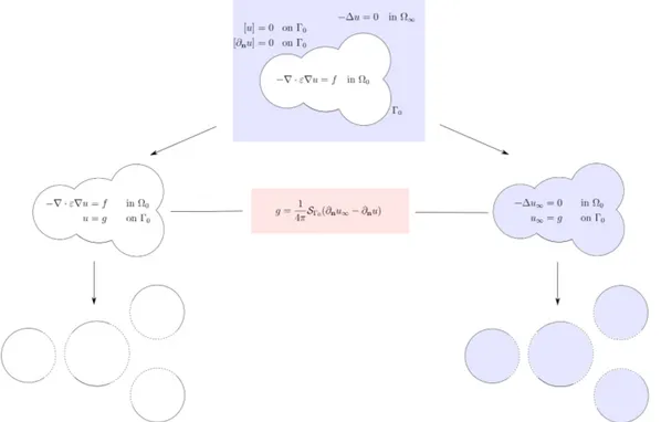
             −∇ · ε∇u = f, in Ω0, −∆u = 0, in Ω∞, [u] = 0, on Γ0, [∂nu] = 0, on Γ0,

where the bounded domain Ω0 and the unbounded domain Ω∞are complementary in

R3_{, [u] and [∂}

nu] denote the jump of u respectively its normal derivative on Γ0 := ∂Ω0.

The scheme of a two-step domain decomposition method for the SES-based PCM (called the ddPCM-SES) is illustrated in Figure 9. The unbounded problem defined inR3 _{is first transformed into two coupled problems both defined on Ω}

0 ® −∇ · ε∇u = f, in Ω0, u = g, on Γ0, and ® −∆u∞= 0, in Ω0, u_∞= g, on Γ0, (3.14)

where the coupling condition arises through the auxiliary variable g defined as

g = 1

4πSΓ0(∂nu∞− ∂nu), on Γ0.

26 3. Domain decomposition methods for implicit solvation models

Figure 8: Schematic diagram of the dielectric permittivity function ε(x) with respect to fsas. The dielectric boundary layer L (switching region) is bounded by two dashed

lines (red), i.e., the region where −rp ≤ fsas ≤ r0.

Laplace equation, SΓ0σ(x) := ∫ Γ0 σ(y) 4π|x − y|, ∀x ∈ Γ0, σ∈ H −1 2(Γ₀). (3.15)

The bounded domain Ω0 is taken as a union of balls, inspired by the geometrical

structure of the solute molecule. Since Ω0 consists of a union of balls, we propose to

further apply a classical domain decomposition algorithm in order to solve the two problems (3.14) by only solving local sub-problems restricted to balls.

As a consequence, a Laplace solver and a Generalized Poisson (GP) solver are developed respectively for solving the Laplace equation and the GP equation in each ball, which allows us to use the spherical harmonics as basis functions in the angular direction to propose an efficient spectral method within each ball. It is important to notice that this algorithm does not require any meshing and only involves problems in balls that are coupled to each other within the domain decomposition paradigm.

In Chapter 3 of Part II, we will present the details of this Schwarz domain decom-position method for the SES-based PCM. We will first remind different solute-solvent boundaries including the VdW surface, the SAS and the SES. We will also provide more details on the construction of the continuous dielectric permittivity function

ε(x) of PCM, ensuring that the SES-cavity always has the dielectric constant of

vac-uum as explained above. Then, we will present the problem formulation of the PCM as well as its equivalent transformation, and therefore, a global strategy for solving the problem. Later, we will introduce the scheme of the domain decomposition method for solving the associated partial differential equations iteratively. This requires to

Figure 9: Schematic diagram of the domain decomposition method for the SES-based PCM (ddPCM-SES).

develop the Laplace solver and the GP-solver in a ball, which are presented. After that, we will give a series of numerical results of the proposed method.

3.4

ddLPB

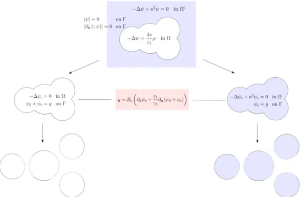
For the sake of simplicity, we focus on solving the linearized Poisson-Boltzmann equation (2.8) defined in R3_{. This problem can be divided into a Poisson equation}

defined in the bounded solute cavity Ω and a homogeneous screened Poisson (HSP) equation defined in the unbounded solvent region Ωc _{as follows}

{

− ∆ψ(x) = 4πρM(x) in Ω,

− ∆ψ(x) + κ2_{ψ(x) = 0 in Ω}c_, (3.16)

combined with two classical jump-conditions

{

[ψ] = 0 on Γ, [∂n(ε ψ)] = 0 on Γ.

(3.17)

Here, κ is the Debye-Hückel screening constant. We remind that the solute cavity Ω in the context of the PB equation consists of a union of balls (i.e., we take the VdW-cavity or the SAS-cavity due to the simple geometry).

28 3. Domain decomposition methods for implicit solvation models

The scheme of a two-step domain decomposition method for the PB solvation model (called the ddLPB method) is illustrated in Figure 10. As in the ddCOSMO, we first homogenize the Poisson equation (3.16), using ψ0 defined by (3.2). The

reaction potential ψr:= ψ− ψ0 satisfies the following Laplace equation {

−∆ψr = 0, in Ω,

ψ0+ ψr = g, on Γ.

(3.18)

Further, we use the integral equation formulation to represent the electrostatic po-tential ψ|Ωc in the solvent region, which simultaneously gives the potential ψ_e of an extended screened Poisson equation in the solute cavity (this is an interior Dirichlet

problem) _{

−∆ψe(x) + κ2ψe(x) = 0, in Ω,

ψe = g, on Γ,

(3.19)

where ψe satisfies the same HSP equation as ψ|Ωc with the same Dirichlet boundary condition on Γ, but defined in Ω. The coupling condition between ψr and ψe arises

through an auxiliary variable g defined as

g =Sκ Ç ∂nψe− 1 εs ∂n(ψ0+ ψr) å , on Γ, (3.20)

where Sκ is another single-layer potential defined as

Sκσ(x) := ∫ Γ e−κ|x−y|σ(y) 4π|x − y| , ∀x ∈ Γ, σ ∈ H −1 2(Γ). (3.21)

At this moment, the initial problem has been transformed equivalently into two cou-pled problems (3.18)–(3.19) both defined on the bounded domain Ω with a coupling condition (3.20). Taking advantage of the fact that Ω is a union of overlapping balls, the Schwarz domain decomposition can be applied to solve these two equations by respectively solving a group of coupled sub-problems each defined on a ball.

Ultimately, a Laplace solver and a HSP solver are developed respectively for solv-ing the Laplace equation and the HSP equation in each ball, which allows us to use the spherical harmonics as basis functions in the spherical direction to propose an efficient spectral method within each ball. Similar to the ddCOSMO, the ddPCM and the ddPCM-SES, the ddLPB does not require any meshing and only involves problems in balls that are coupled to each other.

Remark 3.1. The ddPCM-SES method and the ddLPB method are inspired by

the previous ddCOSMO method and ddPCM method which run impressively fast. The ddLPB has the same computational complexity as the ddPCM.

In Chapter 4 of Part II, we will present the details about this Schwarz domain decomposition method for the PB solvation model. We will first introduce different

Figure 10: Schematic diagram of the domain decomposition method for the PB sol-vation model (ddLPB). Here, ε1 = 1 and ε2 = εs.

definitions of the solute-solvent boundary as in Chapter 3 and also the Poisson-Boltzmann equation defined in the whole space in the case where the solvent is an ionic solution. Then, we will transform equivalently the original Poisson-Boltzmann defined in R3 to two coupled equations both defined on the bounded solute cavity. Next, we will present the global strategy for solving these two coupled equations, using the domain decomposition method. The domain decomposition scheme requires to develop two single-domain solvers respectively for the Laplace equation and the HSP equation defined in a ball. After that, we will give a reformulation of the coupling conditions that should be discretized and consequently derive a global linear system to be solved. We will also present a series of numerical tests about the calculation of the electrostatic contribution to the solvation energy using the ddLPB method.

Molecular Surfaces

Mathematical analysis and

calculation of molecular surfaces

Contents

1.1 Introduction . . . 34 1.1.1 Previous Work . . . 35 1.1.2 Contribution . . . 35 1.1.3 Outline . . . 36 1.2 Introduction to implicit surfaces . . . 36 1.3 Implicit molecular surfaces . . . 37 1.4 Solvent accessible surface . . . 39 1.4.1 Mathematical definitions . . . 39 1.4.2 Equivalence statements . . . 41 1.4.3 New Voronoi-type diagram . . . 47 1.4.4 SAS-area and SAS-volume . . . 49 1.5 Solvent excluded surface . . . 50 1.5.1 Mathematical definitions . . . 51 1.5.2 SES-singularities . . . 53 1.5.3 SES-area and SES-volume . . . 56 1.6 Construction of molecular surfaces . . . 59 1.6.1 Construction of the cSAS and the eSAS . . . 60 1.6.2 Binary tree to construct spherical patches . . . 60 1.6.3 Interior of a loop . . . 62 1.6.4 Construction of the cSES and the eSES . . . 62 1.7 Numerical results . . . 63

34 1.1. Introduction

1.7.1 A system of two atoms . . . 63 1.7.2 Molecular areas and volumes . . . 64 1.7.3 Comparison with the MSMS-algorithm . . . 64 1.7.4 Computational cost . . . 67 1.8 Conclusion . . . 67

This chapter has been published as a journal paper [93]. As mentioned in the introduction of this thesis, we present in this chapter a complete characterization of the Solvent Excluded Surface (SES) for molecular systems, including a complete characterization of singularities of the surface. The theory is based on an implicit representation of the SES, which, in turn, is based on the signed distance function to the Solvent Accessible Surface (SAS). All proofs are constructive so that the theory allows for efficient algorithms in order to compute the area of the SES and the volume of the SES-cavity, or to visualize the surface. Further, we propose to refine the notion of SAS and SES in order to take inner holes in a solute molecule into account or not.

1.1

Introduction

As mentioned in Section 1 of the introduction of this thesis, the majority of chemically relevant reactions take place in the liquid phase and the effect of the environment (solvent) is important and should be considered in various chemical computations. The implicit solvation model (or continuum solvation model) is a model in which the effect of the solvent molecules on the solute are described by a continuous model [109]. In continuum solvation continuum models, the notion of molecular cavity and molecular surface is a fundamental part of the model. The molecular cavity occupies the space of the solute molecule where a solvent molecule cannot touch and the molecular surface, the boundary of the corresponding cavity, builds the interface between the solute and the solvent.

A precise understanding of the nature of the surface is essential for the implicit sol-vation model and as a consequence for running numerical computations. The van der Waals (VdW) surface, the Solvent Accessible Surface (SAS) and the Solvent Excluded Surface (SES) are well-established concepts. The VdW surface is more generally used in chemical calculations, such as in the recent developments [25, 72] for example, of numerical approximations to the COnductor-like Screening MOdel (COSMO) due to the simplicity of the cavity. Since the VdW surface is the topological boundary of the union of spheres, the geometric features are therefore easier to understand. However, the SES, which is considered to be a more precise description of the cavity, is more complicated and its analytical characterization remains unsatisfying despite a large number of contributions in literature.

1.1.1

Previous Work

In quantum chemistry, atoms of a molecule can be represented by VdW-balls with VdW-radii obtained from experiments [97]. The VdW surface of a solute molecule is consequently defined as the topological boundary of the union of all VdW-balls. For a given solute molecule, its SAS and the corresponding SES were first introduced by Lee & Richards in the 1970s [67, 99], where the solvent molecules surrounding a solute molecule are reduced to spherical probes [109]. The SES is also called “the smooth molecular surface” or “the Connolly surface”, due to Connolly’s fundamental work [30]. He has divided the SES into three types of patches: convex spherical patches, saddle-shaped toroidal patches and concave spherical triangles. But the self-intersection among different patches in this division often causes singularities de-spite that the whole SES is smooth almost everywhere. This singularity problem has led to difficulty in many associated researches on the SES, for example, failure of SES meshing algorithms and imprecise calculation of molecular areas or volumes, or has been circumvented by approximate techniques [28]. In 1996, Sanner treated some special singularity cases in his MSMS (Michel Sanner’s Molecular Surface) soft-ware for meshing molecular surfaces [102]. However, to our knowledge, the complete characterization of the singularities of the SES remains unsolved.

1.1.2

Contribution

In this chapter, we will characterize the above molecular surfaces with implicit functions, as well as provide explicit formulas to compute analytically the area of molecular surfaces and the volume of molecular cavities. We first propose a method to compute the signed distance function to the SAS, based on three equivalence statements which also induce a new partition ofR3. As a consequence, a computable implicit function of the corresponding SES is given from the relatively simple relation-ship between the SES and the SAS. Furthermore, we will redefine different types of SES patches mathematically so that the singularities will be characterized explicitly. Besides, by applying the Gauss-Bonnet theorem [35] and the Gauss-Green theorem [38], we succeed to calculate analytically all the molecular areas and volumes, in par-ticular for the SES. These quantities are thought to be useful in protein modeling, such as describing the hydration effects [100, 19].

In addition, we will refine the notion of SAS and SES by considering the possible inner holes in the solute molecule yielding the notions of the complete SAS (cSAS) and the corresponding complete SES (cSES). To distinguish them, we call respectively the previous SAS and the previous SES as the exterior SAS (eSAS) and the exterior SES (eSES). A method with binary tree to construct all these new molecular surfaces will also be proposed in this chapter in order to provide a computationally efficient method.

36 1.2. Introduction to implicit surfaces

1.1.3

Outline

We first introduce the concepts of implicit surfaces in the second section and the implicit functions of molecular surfaces are given in the third section. In the fourth section, we present two more precise definitions about the SAS, either by taking the inner holes of the solute molecule considered into account or not. Then, based on three equivalence statements that are developed, we propose a computable method to calculate the signed distance function from any point to the SAS analytically. In this process, a new Voronoi-type diagram for the SAS-cavity is given which allows us to calculate analytically the area of the SAS and the volume inside the SAS. In the fifth section, a computable implicit function of the SES is deduced directly from the signed distance function to the SAS and according to the new Voronoi-type diagram, all SES-singularities are characterized. Still within this section, the formulas of calculating the area of the SES and the volume inside the SES will be provided. In the sixth section, we explain how to construct the SAS (cSAS and eSAS) and the SES (cSES and eSES) for a given solute molecule considering the possible inner holes. Numerical results are illustrated in the seventh section and finally, we provide some conclusions of this chapter in the last section.

1.2

Introduction to implicit surfaces

We start with presenting the definition of implicit surfaces [112]. In a very general context, a subset O ⊂ Rn _{is called an implicit object if there exists a real-valued}

function f : U → Rk _withO ⊂ U ⊂ Rn_{, and a subset V} ⊂ Rk_{, such that}O = f−1_{(V ).}

That is,

O = {p ∈ U : f(p) ∈ V }.

The above definition of an implicit object is broad enough to include a large family of subsets of the space. In this chapter, we consider the simple case where U =R3_{, V =}

{0} and f : R3 → R is a real-valued function. As a consequence, an implicit object is

represented as a zero-level setO = f−1(0), which is also called an implicit surf ace in R3_{, and the function f is called an implicit f unction of the implicit surface. Notice}

that there are various implicit functions to represent one surface in the form of a zero-level set.

The signed distance function fS of a closed bounded oriented surface S in R3,

determines the distance from a given point p ∈ Rn to the surface S, with the sign determined by whether p lies inside S or not. That is to say,

fS(p) =      − inf x∈S∥p − x∥ if p lies inside S, inf x∈S∥p − x∥ if p lies outside S. (1.2.1)

Figure 1: This is a 2-dimension (2D) schematics of the SAS and the SES, both defined by a spherical probe in orange rolling over the molecule atoms in dark blue.

This is naturally an implicit function of S.

1.3

Implicit molecular surfaces

In quantum chemistry, atoms of a molecule are represented by VdW-balls with VdW radii which are experimentally fitted, given the underlying chemical element [97]. As a consequence and mathematically speaking, the VdW surface is defined as the topological boundary of the union of all VdW-balls. Besides, the SAS of a solute molecule is defined by the center of an idealized spherical probe rolling over the solute molecule, that is, the surface enclosing the region in which the center of a spherical probe can not enter. Finally, the SES is defined by the same spherical probe rolling over the solute VdW-cavity, that is, the surface enclosing the region in which a spherical probe can access. In other words, the SES is the boundary of the union of all spherical probes that do not intersect the VdW-balls of the solute molecule, see Figure 1 for a graphical illustration.

We denote by M the number of atoms in a solute molecule, by ci ∈ R3and ri ∈ R+

the center and the radius of the i-th VdW atom. The open ball with center ci and

radius ri is called the i-th VdW-ball. The van der Waals surface can consequently be

represented as an implicit surface f_vdw−1 (0) with the following implicit function:

fvdw(p) = min

i=1,...,M{∥p − ci∥2− ri}, ∀p ∈ R

3_{. (1.3.1)}

Similarly, the open ball with center ci and radius ri+ rpis called the i-th SAS-ball

denoted by Bi, where rp is the radius of the idealized spherical probe. Furthermore,

we denote by Si the i-th SAS-sphere corresponding to Bi, that is, Si = ∂Bi. Similar

38 1.3. Implicit molecular surfaces

the following implicit function:

e

fsas(p) = fvdw(p)− rp = min

i=1,...,M{∥p − ci∥2− ri− rp}, ∀p ∈ R

3

. (1.3.2)

We notice that the above implicit function of the SAS is simple to compute. It seems nevertheless hopeless to us to further obtain an implicit function of the SES if constructing upon this simple implicit function fesas(p) which is not a distance

function. On the other hand, having the signed distance function, see (1.2.1), at hand would allow the construction of an implicit function for the SES due to the geometrical relationship between the SAS and the SES.

Indeed, according to the fact that any point on the SES has signed distance −rp

to the SAS, an implicit function of the SES is obtained directly as:

fses(p) = fsas(p) + rp, (1.3.3)

which motivates the choice of using the signed distance function to represent the SAS. From the above formula, the SES can be represented by a level set f_sas−1(−rp),

associated with the signed distance function fsas to the SAS. Therefore, the key point

becomes how to compute the signed distance fsas(p) from a point p∈ R3 to the SAS.

Generally speaking, given a general surface S ⊂ R3 _{and any arbitrary point p}∈ R3_,

it is difficult to compute the signed distance from p to S. However, considering that the SAS is a special surface formed by the union of SAS-spheres, this computation can be done analytically.

We state a remark about another implicit function to characterize the SES, pro-posed by Pomelli and Tomasi [90]. In [89], this function can be written as:

e

fses(p) = min

1≤i<j<k≤Mfijk(p), ∀p ∈ R 3

, _(1.3.4)

where fijkrepresents the signed distance function to the SES of the i-th, j-th and k-th

VdW atom. However, this representation might fail sometimes, see two representative 2D examples in Figure 2. Indeed, the formula (1.3.4) for each molecule in Figure 2 can be rewritten as:

e

fses(p) = min

1≤i<j≤3fi,j(p), ∀p ∈ R 2_,

(1.3.5)

where fi,j represents the signed distance function to the SES of the i-th and the j-th

VdW atom. However, each molecular cavity defined by {p ∈ R2 _{: f}e

ses(p) ≤ 0} has

excluded the region in grey inside the real SES.

Further, the region enclosed by the van der Waals surface is called the VdW-cavity, that is, any point p in the VdW-cavity satisfies fvdw(p) ≤ 0. More generally,

we call the region enclosed by a molecular surface as the corresponding molecular cavity. As a consequence, the region enclosed by the SAS is called the SAS-cavity,

Figure 2: The above figures illustrate two SESs of two artificial molecules respectively containing three atoms. In each of them, f1,2 denotes the signed distance function to

the SES of the 1st and the 2nd atoms which is depicted with dashed red curves (f2,3

and f1,3 are similar).

and the region enclosed by the SES is called the SES-cavity. Similarly, any point p in the SAS-cavity satisfies fsas(p) ≤ 0, and any point p in the SES-cavity satisfies

fses(p)≤ 0.

1.4

Solvent accessible surface

In the framework of continuum solvation models, using the VdW-cavity as the solvent molecular cavity has the characteristic that its definition does not depend in any way on characteristics of the solvent. In other words, the above-mentioned VdW surface has ignored the size and shape of the solvent molecules, while the definition of the SAS includes some of these characteristics. In the following, we first provide two more precise mathematical definitions of the SAS considering possible inner holes of a solute molecule. After that, we will provide a formula for the signed distance function to the SAS, which is indeed based on three equivalence statements, providing explicitly a closest point on the SAS to any point in R3_{. In this process,}

a new Voronoi-type diagram will be proposed to make a partition of the space R3_,

which, in turn, will also be used to calculate the exact volume of the SAS-cavity.

1.4.1

Mathematical definitions

In [67], the SAS is defined by the set of the centers of the spherical probe when rolling over the VdW surface of the molecule. At first glance, one could think that it can equivalently be seen as the topological boundary of the union of all SAS-balls of the molecule. However, we notice that there might exist some inner holes inside the molecules where a solvent molecule can not be present. As a consequence, the SAS may or may not be composed of several separate surfaces, see Figure 3 for a