Applied math in geophysical fluids: partially
trapped wave problems and mining plumes.
by
Andrew Joseph Rzeznik
B.S., Cornell University (2013)
Submitted to the Department of Mathematics
in partial fulfillment of the requirements for the degree of
Doctor of Philosophy
at the
MASSACHUSETTS INSTITUTE OF TECHNOLOGY
September 2018
@
Massachusetts Institute of Technology 2018. All rights reserved.
Signature redacted
A uthor ..
...
Department of Mathematics
August 7, 2018
Signature redacted
C ertified by ...
...
Rodolfo R. Rosales
Professor of Applied Mathematics
Thesis Supervisor
Signature redacted
A ccepted by ...
...
Jonathan Kelner
Chairman, Department Committee on Graduate Theses
MASSACHUSETS INSTITUTE OF TECHNOWGY
OCT. 0 2 2 018
MITLibraries
77 Massachusetts Avenue
Cambridge, MA 02139 http://Iibraries.mit.edu/ask
DISCLAIMER NOTICE
Due to the condition of the original material, there are unavoidable
flaws in this reproduction. We have made every effort possible to
provide you with the best copy available.
Thank you.
The images contained in this document are of the
best quality available.
Applied math in geophysical fluids: partially trapped wave
problems and mining plumes.
by
Andrew Joseph Rzeznik
Submitted to the Department of Mathematics on August 7, 2018, in partial fulfillment of the
requirements for the degree of Doctor of Philosophy
Abstract
The first portion of this work focuses on leaky modes in the atmospheric sciences. Leaky modes (related to quasi-modes, scattering resonances, and the singularity ex-pansion method) are discrete, oscillatory and decaying modes that arise in conserva-tive systems where waves are partially trapped. By replacing the infinite domain with a finite domain and appropriate boundary conditions it is possible in many cases to construct a complete basis for the solution in terms of these modes. Formulating such effective boundary conditions requires a notion of the direction of propagation of the waves. For this purpose we introduce a generalization of the concept of group speed for exponentially decaying but conservative waves. This is found via an extended modulation argument and a generalization of Whitham's Average Lagrangian theory. The theory also shows that a close relationship exists between the branch cuts of the dispersion relation and the propagation direction, and is used to create spectral decompositions for simple problems in internal gravity waves.
The last chapter considers deep-sea nodule mining operations, which potentially involve plans for discharge plumes to be released into the water column by surface operation vessels. We consider the effects of non-uniform, realistic stratifications with vertical shear on forced compressible plumes. The plume model is developed to ac-count for the influence of thermal conduction through the discharge pipe and an initial adjustment phase. We investigate the substantial role of compressibility, for which a dimensionless number is introduced to determine its importance compared to that of the background stratification. Our results show that (i) small-scale stratification features can have a significant impact, (ii) in a static ambient there exists a discharge flow rate that minimizes the plume vertical extent, (iii) the ambient velocity profile plays an important role in determining the final plume scale and dilution factor, and (iv) for a typical plume the dilution factor is expected to be several hundred to a thousand.
Thesis Supervisor: Rodolfo R. Rosales Title: Professor of Applied Mathematics
Acknowledgments
This work was supported by NSF grant DMS-1318942, and the Hertz Foundation. Specific to the work on Mining plumes, the stratification data data were collected
and made freely available by the International Argo Program and the national
pro-grams that contribute to it. (http://www.argo.ucsd.edu, http://argo.jcommops.org).
The Argo Program is part of the Global Ocean Observing System. The work on
min-ing plumes was also supported by an MIT Environmental Solutions Initiative seed
grant.
A special thanks to my parents George and Alicja for everything they have done
for me, and to my wife Catherine Howland for being the best partner in life one could
Contents
1 Introduction
1.1 Motivation and description of the research . . . .
1.1.1 Complete Basis of Solutions . . . .
1.1.2 Generalized Group Speed . . . .
1.1.3 Application to Internal Gravity Waves . . . .
1.1.4 Numerical Techniques: Spectral Methods . . . .
1.1.5 M ining Plum es . . . .
1.2 Related and Prior Work . . . .
1.2.1 The mathematical theory of scattering resonances (TSR)
1.2.2 The singularity expansion method (SEM) . . . .
1.2.3 Quasi-Normal Modes . . . .
2 Leaky Modes
2.1 Introduction . . . .
2.1.1 A simple example: the two-speed wave equation
2.1.2 Discrete leaky modes . . . .
2.1.3 Continuous spectrum and natural boundaries
2.1.4 The case with no wave-speed jump . . . .
2.2 A not-so-simple example . . . .
2.3 Branch Cuts and the Complex Dispersion Relation . .
2.4 Energy propagation direction for CEW . . . .
2.5 Application: the two-speed Klein-Gordon . . . .
2.5.1 The Effective Boundary Condition (EBC) . . .
15 . . . 15 . . . 18 . . . 20 . . . 22 . . . 22 . . . 23 . . . 23 . . . 23 . . . 25 . . . 27 29 . . . . 29 . . . . 32 . . . . 35 . . . . 37 . . . . 39 . . . . 40 . . . . 41 . . . . 44 . . . . 46 . . . . 46
2.5.2 The Green's function for the reduced problem . . . . 48
2.5.3 Poles and quasi-modes . . . . 49
2.5.4 Branch cuts and natural boundaries . . . . 50
2.6 Internal Gravity Waves . . . . 52
2.7 Relation to Normal Operators . . . . 54
2.8 Conclusions . . . . 55
3 Group Velocity for Complex Exponential Waves 57 3.1 Introduction . . . . 57
3.1.1 Classical group speed derivation . . . . 58
3.1.2 Whitham's Averaged Lagrangian Theory . . . . 60
3.1.3 Dispersion relation for complex exponentials . . . . 61
3.2 Group speed in the Multi-dimensional case . . . . 62
3.2.1 Modulation Method . . . .. 64
3.2.2 Averaged Lagrangian Method . . . . 67
3.3 Exam ples . . . .. . . . 71
3.3.1 Klein-Gordon Group Speed . . . . 71
4 Mining Plumes 83 4.1 Introduction . . . . 83
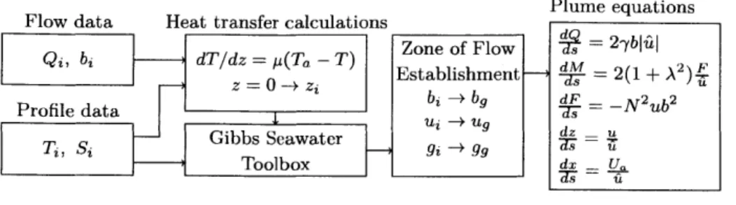
4.2 Plume model . . . . 88
4.2.1 Axisymmetric model equations . . . . 88
4.2.2 Zone of flow establishment . . . . 92
4.2.3 Compressibility and Thermodynamic considerations . . . . 93
4.2.4 Plume parameters and initial conditions . . . . 97
4.2.5 Practical pipe flow considerations . . . . 101
4.3 R esults . . . . 105
4.3.1 uniform stratification results . . . . 105
5 Conclusion and discussion
5.1 Ocean Gravity W aves . . . . 115 5.2 M ining plum es . . . . .. . . . . 116
A Green's functions for the simple two-speed wave equation
119
B Leaky mode expansion for an atmospheric toy model
121
List of Figures
1-1 The first few modes for the two-speed wave equation . . . . 19
1-2 Location of the spectrum (poles/discrete and branch cuts/continuous) for a few simple examples of interests in applications . . . . 26
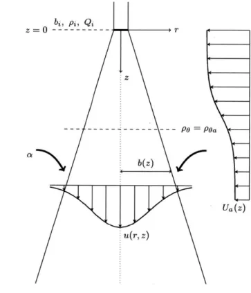
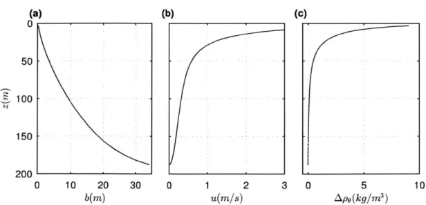
4-1 Schematic illustrating the axisymmetric plume model . . . . 88
4-2 The potential density and derivative along with the ambient velocity, for an example averaged ocean stratification . . . . 97
4-3 Schematic of the solution process for the plume calculation . . . . 103
4-4 Temperature and density anomalies for an example plume . . . . 104
4-5 A-dimensional solution for a plume with a uniform stratification . . . 105
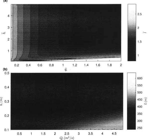
4-6 Plots of plume vertical extent compared to the initial flow rate and radius for a uniform stratification . . . . 107
4-7 Dimensional solution for an example plume . . . . 108
4-8 Plume extent as a function of various parameters . . . . 109
4-9 Plume vertical extent and final absolute depth, as functions of the release depth . . . . 111
4-10 Plume end parameters as functions of the release depth . . . 111
4-11 Plume end parameters vs. ambient background velocity . . . . 112
List of Tables
Chapter 1
Introduction
1.1
Motivation and description of the research
The main interest of the first portion of this thesis is investigating problems where
(linear) dispersive, conservative, waves are trapped by a partially reflecting boundary, beyond which they are allowed to radiate to infinity. Such problems are very common
throughout the physical sciences. A common example is that of light rays in a piece
of glass (or in an optical fiber), which can be either partially or completely reflected
at the glass-air interface - depending on the incidence angle. However, problems
like this are not exclusive to electromagnetic waves. Acoustic systems can also
ex-hibit partial trapping at boundaries, such as sound waves reverberating in a tuning
fork, while also escaping into the surrounding air. Likewise, internal gravity waves in
geophysical systems can be trapped through partially reflecting boundaries - e.g., atmospheric internal waves in the troposphere; see section 1.1.3. In many such
sys-tems, one may only care about what occurs within the partially reflecting boundaries, with the solution in the external region (the outside media for a wave-guide or the
stratosphere for atmospheric internal waves). This then raises the natural question:
can one pose appropriate "Effective boundary conditions" (EBC) at these boundaries, to reduce the problem to a finite domain? Further: what is the behavior of the result-ing "reduced" system? In particular, how is the spectrum (discrete or continuous) of the problem related to the presence of a partially reflecting boundary?
Formulation of an EBC requires first a Reflection-Transmission Coefficient (RTC) calculation at the boundary, with the EBC then defined so as to reproduce the so obtained Reflection Coefficient without the outside media. The crucial step in a RTC calculation is knowing in which direction the waves propagate. In classical dispersive wave theory this is provided by the group velocity. However, due to the energy loss through the boundaries, the solutions in the finite region will generally decay in time, and cannot be properly expanded in terms of purely sinusoidal waves, I as the classical dispersive wave theory assumes. Hence the classical notion of group speed cannot be used, and a generalization is needed - for more details see subsection 1.1.2.
This thesis derives a generalization to the notion of group speed appropriate for conservative systems which lose energy to infinity at partially reflecting boundaries. This generalized group velocity theory is developed using both modulation theory, and an adaptation of Whitham's Average Lagrangian theory [81]. The theory is used to formulate EBC. We show that the natural way to pose the EBC is through the Laplace Transform formulation of the problem. Using the EBC, the Green's function for the Laplace Transform (i.e.: the resolvent operator) can be constructed. Through the inverse Laplace Transform formula, the singularities of this Green function lead to a spectral decomposition for the reduced problem: the Leaky Spectrum. In particular, when only poles occur, a Leaky Modes expansion of the solution can be obtained. The modes are called "leaky" because they naturally incorporate the energy loss at the boundary, and exhibit exponential decay in time. An application example, internal waves in the troposphere, is developed in detail - see chapter 2.
For a concrete, simple, initial example, consider the initial value problem for the wave equation on an infinite line, x E R,
utt
-
uXX + V(x) u = 0, u(x, 0)
=f(x),
(1.1)
where both the potential and the initial conditions are compact: V E C (R) and
1 To be precise: almost anything can be expanded in terms of sinusoidals (i.e.: Fourier series). But the convergence of such expansions near the boundary would be extremely poor, because such solutions would not satisfy the proper radiation conditions. Hence trying to use such solutions to formulate EBC is a highly unreliable process.
f E CO (R). The Laplace Transform, via its inversion formula, provides a spectral formula for the general solution to this problem (integral/sum over the singularities
of the transform in the complex plane). In order to avoid having to switch back-and-forth between the frequency A and the Laplace variable s, related by
s = -i A, (1.2)
the (fully equivalent) "one-sided" (time) Fourier Transform
00
is often used. Then the problem above takes the form
(-2
+ V(x) -A
2)i = g(x), VE
C, (R), xE
R, (1.4)with the radiation condition
S=RtgAx for sg X > XO, (1.5)
where s9 = 1, and x0 > 0 is some constant. This condition ensures that beyond
some compact region only waves radiating away to infinite are present.
For the problem above (both in ID and in the analog multi-dimensional problem)
it has been rigorously shown that the asymptotic t -> oc behavior can be described
as a sum of a discrete set of modes, each with complex frequency leading to both
decay and oscillation in time [42].
Systems which are locally conservative, but radiate energy away to infinity, arise
in many scattering problems, as well as in some situations which traditionally would
not be considered scattering problems. This thesis attempts to bring these separate
applications into a single consistent framework, and adds to the theory several
numer-ical and analytnumer-ical results. On the analytnumer-ical side it is shown that for many cases the
series is not just a long-time asymptotic approximation, but exact for all time when
suitable written. Furthermore, the theory is generalized beyond dispersion-less wave
general dispersive systems. This, specifically, for problems where there is a boundary
beyond which the system is a linear, dispersive, constant coefficients pde. It is then
shown that the construction of a proper scattering solution is best done through the
use of a complex group velocity, which ensures that the proper radiation condition at
the boundaries is satisfied. Applications are considered in geophysical fluid dynamics, where there have been minimal attempts to use scattering expansion techniques, but
where there are many problems which naturally fall into their domain.
1.1.1
Complete Basis of Solutions
One of the objectives of the work in this thesis is the formulation of Effective
Bound-ary Conditions (EBC) for dispersive/conservative problems with partially reflecting boundaries beyond which the waves radiate to infinity, and never return. This then
reduces the problem to one which can be solved in the region of physical interest
only. For many such reduced systems a complete basis of solutions can be found. A
simple example is that of the two-speed wave equation (i.e.: c2
is one constant for
0 < x < 1, a different constant for 1 < x < oc, and Dirichlet BC apply at x = 0).
Figure 1-1 shows the first five modes of the complete basis (here the spectrum is
purely discrete) for this example. Other examples arise in models of the atmosphere see chapter 2. The irrotational internal wave equation with a "leaky boundary"
exhibits behavior somewhat similar to the two-wave equation, while the addition of
rotation requires continuous spectrum - which arises from the contributions from a branch cut. This second example is similar in this respect to the Klein-Gordon
equation with a piece-wise constant potential.
Remark 1.1 [Relationship between branch cuts and the generalized group speed]. The prior paragraph requires some clarification: generally the location of a branch cut is not uniquely determined. On the other hand, the following
loca-tions are uniquely determined: (a) (complex) wave-frequencies corresponding to a
vanishing group speed; (b) continuous spectrum; and (c) (complex) wave-frequencies
06
-0-4
0-2
-0.2
0 0.1 0.2 0.3 0-4 0.5 0.6 0.7 0.8 0.9 1
Figure 1-1: The first few modes for the two-speed wave equation, described in the text. For two constant speeds (one inside and one outside the domain) they are given by general hyperbolic trigonometric functions, which are the natural complex-wavenumber analog to the sine and cosine modes that arise for 1-D constant coefficient
conservative problems.
locations coincide, and they also determine the appropriate place where the branch
cut for the Green's function of the resolvent operator must be placed.
44
It is important to note that the spectral theory for the solutions mentioned above is
valid only for the reduced problem. That is, it can be used to represent the solutions only up to the boundary where the EBC are imposed, but not beyond - in fact, the
eigenmodes typically blow up as jx -+ oc, so that the basis does not make physical
sense beyond the effective boundary. Furthermore: the reduced problem is, typically, not normal (because of the nature of the EBC, which are both non-local, and include
time dependence). Yet, through the use of the Green's function for the Laplace
Transform of the problem, and its inversion formula, a spectral representation can be
obtained.
Remark 1.2 [Partial containment is crucial]. In order to actually get leaky modes a region of space from which the energy leaks, but only partially, is crucial. A
"trans-parent" boundary does not work. In particular, this means that one cannot
"artifi-cially" impose a boundary somewhere (such as is done in numerical computations to
reduce an infinite domain to a finite one), and expect to get a base of leaky modes.2 2This is somewhat unfortunate, because it means that there is no readily available set of functions that could make the calculation more efficient or accurate.
The boundaries, if there, are physical features of the problem itself.
To understand why this is so, consider that a leaky mode, by it very nature, must decay, and do so exponential. A wave bouncing back and forth in a box, losing some fraction of its energy at every bounce, will produce exponential decay. Of course, to get an actual "mode" more is needed: the bounces must be coherent, so that the space configuration repeats after each cycle. On the other hand, if there is no box (transparent boundaries), then the wave just exits and is gone.
This argument is, of course, not a proof. Hence there exists the possibility of some special case where the statement made here might fail.
4
1.1.2
Generalized Group Speed
In order to formulate an Effective Boundary Condition (EBC), the direction of propa-gation for the information/energy is needed. For hyperbolic problems this follows from the characteristics. For dispersive systems the question becomes more complicated, as it must be addressed "wave-by-wave". When the solution can be decomposed into
sinusoidal waves e (kiwt) (with k and w = w(k) real), the classical notion of group
speed, ' = Vk w, provides the answer. However, the systems of interest to us (even
though conservative) have decay due to the energy losses through the boundaries. Hence the solutions to the reduced equations (inside the boundaries at which the EBC apply) cannot be decomposed in terms of exponentials with a real wave-number and a real wave-frequency. Instead "Complex Exponential Waves" (CEW) are needed, proportional to
e:+s
,(1.6)where d is a complex vector, and s is a complex number - related to d through a complex dispersion relation. ' Thus a generalization of the notion of group speed to
solutions of the form in (1.6) is needed. This is done in this thesis, where we show
that the correct object is the generalized group speed, c , defined below.
The generalized group speed,
c.
3
The use of the notation s for the generalized frequency is not accidental. The expression in (1.6) arises naturally when the solutions are written in terms of an inverse Laplace Transform.
If Re(d) 0, then (because the system is dispersive) s is purely imaginary, and (1.6)
has the form eZi k-'V (with
i
and w = w(k) real). Hence the classical theory applies and C' = Vk w. Thus, assume Re(d) $ 0, and write: d= mn
+
i k and s = - - LO where {m, h , k, , w} are real, h is a unit vector and m 4 0. Thenand ()'= (Vk ) , (1.7)
m
where I is used to indicate the component orthogonal to ft. Note now that
1. These formulas are consistent with the classical group speed, and reduce to
them when m -> 0. This is clear for (' )1, and a simple calculation in chapter
3 shows that the same is true for h -Cg.
2. The formula for (')- suggests that this component is the same as in the classical case. But it is not, because here L = w (Re(d), k), and V is taken at a point where Re(d) $0.
3. The CEW in (1.6) has the form emti+Ot+iO, where 0 = k - - o t. Thus it is an oscillatory sinusoidal wave, with an exponential envelope emflx+at propagating at speed -- /m along the direction given by h.
Remark 1.3 [Dissipative media]. Ascertaining the direction of propagation of in-formation/energy for waves in dissipative media is a related research area [68, 26].
Here real frequencies naturally lead to complex wave-numbers and, vice versa.
How-ever, the two problems are different (both physically, and mathematically). In this
second problem the waves lose energy to the media (e.g.: wave energy gets converted
into heat). Further, for a sufficiently large dissipation, propagation ceases. By
con-trast, in our problem some energy leaves the system through the boundary, but there
are no losses inside the system, and propagation is not hampered. Furthermore, both
the wave-number and the wave-frequency are complex simultaneously - the only exception being the evanescent waves, which exactly correspond to the distinguished
1.1.3
Application to Internal Gravity Waves
A main goal of this thesis is to apply the methods described above (effective boundary conditions, generalized group velocity, and leaky modes) to problems in geophysical fluid dynamics, in particular to those dealing with internal gravity waves. While there has been some research on using radiation boundary conditions in geophysical fluids [531, there has been little research into analyzing the spectrums that arise from such conditions. The first application of leaky modes occurred in
[131,
where it was termed a leaky-lid expansion for eigenmodes of internal waves in the troposphere. The rapid change in the stratification gradient between the troposphere and the stratosphere, combined with the fact that essentially no internal atmospheric waves are reflected back into the troposphere from the stratosphere, allows the formulation of EBC. The only other work using such methods is179],
where initial atmospheric tsunami waves were projected onto leaky modes in order to analyze their transient decay in time with appropriate radiative boundary conditions. As far as the author is aware, the work cited above is the only work in atmospheric research using Effective Boundary Conditions, Leaky modes, or related methods. In this thesis we both (i) extend this work, to produce a more rigorous and general framework, and (ii) use the techniques on further applications, which are beyond prior developments, as they include branch cuts - branch cuts are the reason the work in [131 had limited success in dealing with the (very important) effects from rotation.1.1.4
Numerical Techniques: Spectral Methods
The leaky modes expansions (more generally, leaky spectral representations) provide a way to write the exact solution to a problem inside the boundaries at which the EBC apply. This gives rise to the question: Is it possible to use these representations
as the basis for a spectral method? Of course, one can argue that we can produce
explicit leaky spectral representations for relatively simple problems only (e.g.: piece-wise constant coefficients on simple geometries). But this is true as well for the standard spectral methods. In fact, to get around this limitation, techniques have
been developed to decompose complicated geometries into groups of simple
compo-nents interacting at their boundaries [56]. Then a simple spectral basis is used in each
component. In principle there is no reason why leaky spectral basis could not be
incor-porated into this set-up. This could provide an alternative to the Perfectly Matched
Layers (PLM)
[4]
technique used for radiating problems, at least in some cases where physical, partially reflecting boundaries exist. This thesis lays groundwork towardsthis grand goal of new spectral methods for radiating boundary conditions.
1.1.5
Mining Plumes
The last part of this thesis takes a very different direction and builds up a model of
de-watering plumes for deep-sea mining operations. In a deep-sea mining operation, a
seafloor based vehicle retrieves nodules and sediment, some of which is brought to the
ocean surface for processing [551. Waste sediment and other mining debris must then
be returned to the ocean floor. For this final process a return pipe is proposed, which
would extend some distance below the ocean surface and serve as a discharge point.
As any large scale mining operation would be continuously discharging large amounts
of sediment, the depth of the pipe and characteristics of the return plume become
serious considerations for both safety and environmental reasons. Here the plume
characteristics are investigated for a sediment-laden discharge plume in a buoyant
environment, with the goal of understanding the final sediment distribution and the
factors that play a role in determining it.
1.2
Related and Prior Work
1.2.1
The mathematical theory of
scattering resonances (TSR)
In the Analysis literature, the poles of the Green function for a radiating problem
are called Scattering Resonances, and are primarily studied for the case of the
corre-sponding in "one-sided" Fourier space to
- V2u + V(x)u - 2U = 0, x E R'. (1.8)
Such equations are hyperbolic outside the support of the potential and thus allow
and easy definition of outgoing waves. These equations are a compact perturbation
(given by the potential V) to the wave equation, for which much is known. Thus many
nice results about the asymptotic structure of the poles can be proved, such as: (i)
the analytic continuation of resolvent is meromorphic, and (ii) the poles/eigenvalues
asymptotically move away from the real axis as the frequency grows. Using these
results, and others, the long time asymptotic behavior of the solution can be
char-acterized in terms of a series of the residues of the Green function. It also known
(though largely not emphasized) that these series are exact when a cutoff function
is applied, i.e. the series is considered only over a compact region in space. This
exactness offers the promise that scattering resonance methods can provide exact
expressions for problems where the wave field is only desired in a compact region.
An important focus of the mathematical theory of scattering resonances arises
from semi-classical analysis [85], which provides a mathematically rigorous version
of the correspondence principle between quantum and classical mechanics - i.e.: a rigorous WKB method. Semiclassical analysis leads to systems with a different type
of resonance, but which can be studied with the same mathematical tools
[8].
In this context structures known as open quantum maps154,
21] arise, which exhibit their own form of resonance. All these systems include resonances which decay as energyis lost somewhere via radiation.
The resonances of the perturbed Laplace operator on hyperbolic surfaces [5] is another related area of interest in analysis. These questions can often be attacked
relatively rigorously, but only partially and leaving many open questions. In fact, the Riemann Hypothesis can be restated as a question about the absence of
scatter-ing resonances in a strip of the complex plane for a particular hyperbolic scatterscatter-ing
A rigorous mathematical theory for scattering resonances where the resolvent can not be meromorphically continued into the lower A-half plane (left s-plane for the Laplace Transform) has been elusive. For many equations of physical interests, this is precisely the case, with branch cuts and other non-trivial singularities appearing. 4
For example, consider the following slight modification of the iD problem in (1.1), whereby the equation reduces (at large distances) not to the wave equation but the Klein-Gordon equation,
Utt - UXX + V (x) u+ y u = 0, V E C (R), x E R, t E [0, OC), it > 0,
(1.9)
with initial conditions as in (1.1). The introduction of the new term Pu is equiva-lent to replacing the requirement V(x)
C
C((R) in (1.1) by V'(x)C
C (R). Thisno longer satisfies the hypotheses required to prove that the Green function has a meromorphic continuation, which in fact it does not. We will show this later, by solving the problem analytically for some special cases of interest, where one can see that branch cuts appear in the spectrum. More generally, we will show that, for local differential operators, the branch cuts correspond to contributions from evanescent waves, which have a real frequency and do not decay. Moving to a different branch through such a cut corresponds to switching the wave's direction of propagation (in-coming to outgoing solutions, or the reverse). Hence the location of the branch cuts is exactly where the generalized group speed (to be defined later) vanishes. Figure 1-2 illustrates this with plots of the location of the spectrum (poles/discrete and branch cuts/continuous) for several examples where the potential V (or its equivalent) is constant in an interval, and vanishes outside of it.
1.2.2
The singularity expansion method (SEM)
The singularity expansion method, introduced by C.E. Baum [2], provides a way to compute the (decaying) eigenfunctions associated with the dominant resonant poles, and uses them to analyze/describe the asymptotic behavior of the solutions. The SEM has been primarily focused on electromagnetic wave problems from its early
Wave Equation Laplace Domain
.1 ... ... ...
Real
Inktal Waves Laplare Domain
A8
Real
-0.5 0
10
Figure 1-2: Location of the spectrum (poles/discrete and branch cuts/continuous) for
a few simple examples of interest in applications. In each case the mathematical model is a pde with piece-wise constant coefficients. The details behind these examples will be described later in chapter 2 and Appendix A.
inception, and has been used to analyze the transient electromagnetic field created
by radar backscatter off flying objects (with the goal of improving target recognition).
In this case the perturbation to the constant ambient background is a conductor of a
particular shape, e.g.: the metal frame of an airplane. However, the focus here is on
the wave field external to the compact domain, as the objective is to compute the back scatter. Thus no complete "leaky-basis" to expand the solution is obtained; instead
the result is only valid asymptotically. The SEM is important for showing that, even
in cases where the localized perturbation is a perfectly reflecting conductor, discrete
modes can arise in the external field (though they only asymptotically describe it). The SEM has also been used for the analysis of internal transient modes in
waveg-26
Kllin Gordon Laplace Domain
15
10
.10
405 0 0'5
Real
Internal Waves w/ Rotation Laplace Domain
0,8Uandi CuI 084 0,2 402 -.4 -0,8 -2 51 -1 -0 6 0 Real
E
I1 0 -0. -2 i Euides and resonators 164]. This work is also focused on the long time asymptotic
be-havior of the solutions, just as the theory of scattering resonances - see section 1.2.1. However, in many cases the expansions derived should work for all time if the
con-tributions from the branch cuts (often present), or other singularities, are properly
accounted for. In this thesis we develop methods for doing this, and consider
situa-tions of this type that arise in Geophysical Fluids. Then we show instances where it
is possible to derive methods that yield the solutions for all time.
1.2.3
Quasi-Normal Modes
.
Quasi-normal modes are very related to scattering resonances, leaky modes, and the
singularity expansion method; and precede all of them. The notion can be traced back
to the phenomena of Landau damping 141, 7j in plasmas. For an appropriately for-mulated problem, Landau damping corresponds to the slowest decaying leaky mode;
equivalently: the scattering resonance pole for which Re(s) < 0 has the smallest value - see (1.2). More generally, quasi-normal modes correspond to the slowest decaying
leaky modes (i.e.: the dominant resonant poles) in problems where energy is radiating
away to infinity from some form of localized perturbation in an ambient media that
provides only partial containment (see remark 1.2).
In physics quasi-modes are often used to simplify and understand problems with
energy radiating to infinity. In particular, they have been used to study a
black-hole ring-down [16, 20, 39, 841, where its deviations from a spherical shape undergo
damped oscillations until they vanish. Leaky waveguides
[281
have also been analyzed using quasi-modes. In some cases quasi-normal modes have been used to produce aspectral decomposition, e.g.: for optical cavities
[43,
44].Finally, it is worth pointing out that the notion of Green's function used within
the context of the theory of quasi-modes is somewhat different from the one used here, with the poles/resonances being found by deforming the branch cut contours to pick
them up from another sheet. As pointed out in remark 1.1, in our work (at least in
1-D) the branch cuts are uniquely determined by the location where the generalized
set of all the waves moving in a particular direction, either right or left.
Example 1.1 [The simplest example of quasi-normal modes]. Consider a
semi-infinite taut string in a plane, attached to a mass-spring system at the origin, where
the mass can move in the direction normal to the string. The (linear) a-dimensional
equations are Utt - U = 0 for x > 0, with j + ky = ux, (1.10)
where u = u(x, t) is the normal deviation of the string from equilibrium, the su-perscript 0 indicates evaluation at x = 0, y = uO = u(0, t), and k > 0 is the
spring constant. It is easy to check that this system is conservative, with energy
E =
1j
'(u2 2+ u) dx + _(y2+
k y2).The radiation condition here is ut + ux = 0 for x > 0. Implementing this at x = 0
gives the "Effective Boundary Condition" =
and the "reduced system"
+
y
+ ky = 0, (1.11)which, for this simple example, is just an ode. The
"leaky modes" are then y, = eAnt, where the A, are the solutions to A2 + A + k = 0.
Note that, provided k
$
1/4, the leaky modes are a base of solutions for (1.11). The general solution to (1.10), plus the radiation condition (which restricts theinitial data) is then
u=y(t-x) for t>x and u=u(x-t, 0) for t <x. (1.12)
Finally, note that, for t > x, the solution is a linear combination of eA1 (-) and
eA2 (). These are the "quasi-modes", given this name because they are not actually
modes - they grow exponentially as x -+ oc, because Re(An) < 0. Note that, at any given x, if t is large enough, the solution is represented by the quasi-modes.
4
Chapter 2
Leaky Modes
2.1
Introduction
The propagation of waves in linear, translational invariant, dispersive systems is well
understood. It is described by a well developed theory [15, 40, 81, 45] with roots
that go back to the XIX century [61, 69]. The theory is based on sinusoidal profiles
which have a real wave-number k and a real wave-frequency w, related by a dispersion
relation (whose solutions w are real for any real k). One of this theory's key objects
is the group speed, C = Vkw, the speed at which wave energy propagates.
As explained in chapter 1, there are situations where sinusoidal waves with real
wave-number and wave-frequency are not appropriate - even within the context of
dispersive, conservative, systems. These situations require an extension of the
"clas-sical theory" to the case where the wave-number and wave-frequency are complex. 1
Problems in domains with boundaries through which some of the energy is radiated
away are the example of these scenarios that motivate this work. Then, because
of the losses, the wave-frequency cannot be purely real. But then neither can the
wave-number - because, in a conservative system, the dispersion relation yields a real wave-frequency for any real wave-number. In these circumstances the following
considerations arise
'Note that dissipative, non-conservative, systems give rise to such solutions as well, but these are not the focus here. See remark 1.3.
(a) While it might still be possible to write the solutions in terms of standard
Fourier modes (i.e., waves with k and w real), such representations would be
far from optimal (poorly convergent), since the Fourier basis will generally fail
to satisfy the radiation boundary conditions - e.g., see remark 2.4.
(b) Boundary conditions through which radiation is lost often arise when the media
beyond some boundary (e.g., the edge of some optical conductor) is replaced by
a boundary condition. This requires a calculation involving incident, reflected, and transmitted waves at the boundary, followed by the construction of an
Effective Boundary Condition (EBC) - designed so that the reflected waves it produces are equal to those predicted by the previously obtained reflection
coefficient.
Reflection-Transmission coefficient calculations require knowledge of the
direc-tion of propagadirec-tion of the informadirec-tion carried by the waves. This informadirec-tion
is typically obtained using the group velocity provided by the classical theory.
But there is an inconsistency in this process: as explained above, in the
pres-ence of boundary losses, one cannot assume waves where both the wave-number
and the wave-frequency are real. Thus a generalization of the classical theory
is needed.
(c) Item (b) above involves a subtle issue, related to the construction of an EBC.
Examples presented later in this thesis will illustrate this, but the key to the
problem is that the EBC should be such that the reflected waves it produces are
equal to those predicted by the previously obtained reflection coefficient. This often requires pseudo-differential operators which involve either time or the
direction perpendicular to the boundary. Both have unsatisfactory features:
in the first case (time) the resulting set of equations is no longer an initial
value problem (it is global in time), even if the original problem was one. In
the second case, Fourier modes give a poorly convergent representation of the
operator, which makes dealing with it rather difficult. In fact, the optimal representation is the one given by the modes of the reduced problem, which
circular reasoning.
(d) The construction of an EBC by itself is not what triggers a leaky spectral
decom-position (in particular, leaky modes). Instead, as explained in remark 1.2, this arises from a physically inherent property of wave systems which are compact
perturbations (causing partial trapping) to infinite space. The simplest way to
understand this is to consider what happens if one attempts to use an effective
boundary condition for the wave equation in free space, specifying an arbitrary
compact domain across whose boundary waves exit to infinity (full transmission
without any reflection). Without any localized potential, or partially reflective
boundary conditions, in the problem leaky modes need not arise, leading to a
degenerate "reduced" problem without spectrum. A technically more detailed
description, for a model problem, can be found in 2.1.4. Other authors have
also pointed out that the quasi-modes/scattering resonances are related to
fun-damental physical parameters of locally perturbed systems
1751.
The key thing to note is that the leaky spectral representations are not just a convenient wayto expand the problem solutions, but are based/incorporate the fundamental
underlying physics and geometry of the problem.
The purpose of the research described in chapters 2 and 3 is to address these issues.
We will show how to generalize the notion of group speed to complex exponential
waves, how to formulate EBC in a consistent fashion using the Laplace Transform, and how to use this formulation to obtain mode expansions consistent with the EBC.
The group speed found for complex exponential waves agrees with the standard result
in the classical limit (i.e., as the frequency and wave number become real) and for
evanescent waves. The theory also provides a physically meaningful way of placing
the branch cuts in the complex dispersion relation (when the direction of propagation
switches). This so placed branch cuts then correspond to the evanescent waves.
The rest of this chapter is organized as follows. In 2.1.1 we introduce a simple
example to illustrate some of the basic leaky mode concepts, and obtain its leaky mode
expansion. The results from this example are examined in 2.1.2, 2.1.3, and 2.1.4.
we first study the complex dispersion relation for the problem, which includes branch points, in 2.3. We consider the structure symmetries introduce into the solution branches corresponding to right-left moving waves, and use them to obtain the wave propagation direction for CEW. In 2.4, we use the conservation of energy equation to study the energy propagation in 1-D for complex exponential solutions (CEW). A generalized group speed notion is introduced. In 2.5 the ideas developed in 2.4 are applied to the example in 2.2. Then: In 2.5.1 an effective boundary condition (EBC) is developed and the reduced problem is formulated. In 2.5.2 the Green's function for the reduced problem is calculated. In 2.5.3 and 2.5.4 the singularities of the Green's function, and their relationship to the spectrum of the reduced problem, are studied. In 2.6, with the tools developed up to this point, we approach the problem of internal gravity waves in the atmosphere. In 2.7 we consider the relationship of the leaky-mode expansions to normal operators. Finally, 2.8 has the conclusions.
2.1.1
A simple example: the two-speed wave equation
For a simple example that illustrates some of the basic ideas in this thesis, consider the initial-boundary value problem (IBVP) for the "two-speed" wave equation in the half line x > 0. The a-dimensional form of the problem, where the wave speed near the origin is normalized to c = 1, is
utt -c 2
(X) uXz = 0, with u(x, 0)=
f
(x)
and ut(x, 0)=
g(x), (2.1)boundary condition u(0, t) = 0, and wave speed
c(x) = 1, (2.2)
co, X > 1 (0 < co < 1 a constant).
Furthermore, at the discontinuity of c we impose the conditions: u and ux are
contin-uous at x = 1. Finally, we assume that the initial values
f
and g have their support within the interval (0, 1). Note that the case co > 1 is only slightly more complicated than the one treated here, and very similar. But co = 1 is special - see 2.1.4.Note that the initial conditions are such that no information from the region x > 1 moves into the region x < 1. This is actually the key condition that we need for this
problem, and could be achieved (for general
f
and g) by imposing the restrictiong(x) + co f'(x) = 0 for x > 1. (2.3)
Now we have (a) All the waves to the right of x = 1 move to the right, that is ut
+
co ux = 0 for x > 1. (b) u and ux are continuous at x = 1. Using these twofact we can write an IBVP that allows us to solve for u in the region 0 < x < 1 only. That is, the reduced problem
Utt - UX = 0, with u(0, t) = 0, ut (1, t) + co ux (1, t) = 0, (2.4) and initial data: u(x, 0) = f(x) and ut(x, 0) = g(x). Notice that the EBC at x = 1,
Ut
+
co ux = 0, includes a time derivative. This EBC mimics the presence of the media beyond x > 1, and causes incident waves from the left to only partially reflect - themissing energy being what should be transmitted across the discontinuity in c.
The wave equation is very simple, in that it allows an EBC to be written as a
differential boundary condition. The general situation for dispersive systems is more
complicated, because then the EBC is frequency dependent - see 2.2. In fact (2.4)
is simple enough to allow an explicit exact solution, starting from the fact that any
solution to the wave equation has the form u = ur(x - t) + ul(x + t), for some single variable functions ur and ul. Specifically, let 0 < v = - In ( 1icO). Then
u = v(t - x) - v(t + x), where v( ) = e-" 0() (2.5)
Here b is periodic of period 2, defined for > -1, and can be computed if v(x) is known for -1 < x < 1. This follows because the initial conditions yield
v(sg x) =-s - f W + - g(y) dy + f(1), (2.6)
2 2 X 2 co
where 0 < x < 1 and sg = 1. The constant of integration - f(1) is selected to guarantee continuity of b at ( = 1 (provided f is continuous). Continuity at c = 0
follows if f(0) = 0 - i.e., the initial data satisfies the left boundary condition.
Finally, an expansion of the solution in terms of a complete basis of discrete leaky
modes can be obtained by expanding b in a Fourier series - note that the leaky
modes are not purely sinusoidal because they follow from
4
via (2.5). However, this approach is special to this example, and not generalizable. 2 It is more instructive toobtain the solution using the Laplace Transform U = U(x, s) of u. Then
s2 U(x, s) - U22(X, s) = s f(x) + g(x) = y(x, s), (2.7)
with boundary conditions U(0, s) = 0 and s U(1, s) + co Ux(1, s) = f(1), where y
defined by the second equality. Thus
/If(1)
sinh(s) (2.8U =jG(x, y, s) >(y, s) dy + . , (2.8)
sinh(s) + co cosh(s) s
where G is the Green's function for (2.7). Then, using the inverse Laplace Transform
formula, and standard complex variable techniques (see appendix A), yields
U
= fn + - gn + ()f
(1) eSt sinh(sn X), (2.9)E ( s- V1
-nuJ oc(f Sn 2f(1
where Sn -v
+
in7r,fn
- sinh(sn X) f (x) dx, and gn = - sinh(sn X) g(x) dx. (2.10)Remark 2.4 [On Fourier series]. We will now use this example to illustrate the point made in items (a) and (c) at the beginning of this chapter. Suppose that we
at-tempt to solve (2.4) by using a Fourier series for u. Then the left boundary condition
suggests that we should use a sine-Fourier series in 0 < x < 1. Thus, to satisfy the
equation, u = 'cPn(t) sin(n 7r x), where Pn = an cos(n 7r t) + bn sin(n 7r t). There-fore 0 = lim, I (E ,bn(t) sin(n 7r x)
+
co E n 7rnM(t)
cos(n rF x)), from the right boundary condition. However, elucidating what this means in terms of theexpan-sion coefficients is now an uphill task, because the series cannot generally converge
pointwise at x 1 (this would mean that u vanishes there). Using other Fourier
expansions leads to similar, or worse, problems. 4
2.1.2
Discrete leaky modes
Equation (2.9) is an expansion in terms of eigenmodes for the reduced problem (2.4).
That is, solutions to the eigenvalue problem resulting from separating u = eA t (x), which leads to:
A
2 t-
f"=1 0 forO<x<
1, it(O)=0,
and Aii+coit'=O. (2.11)The eigenvalues are A = so, with corresponding eigenfunctions ^n = sinh(s, x). Note that:
(1) This is a peculiar eigenvalue problem, where the eigenvalue appears not just in
the equation, but also in the boundary conditions. As we will see later, this is
typical for problems where there are radiation losses through a boundary. We
will call normal modes arising in situations of this type leaky modes, though in
other fields they are also referred to as quasi-modes or scattering resonances.
(2) Because Re(sL) = -v < 0, the modes decay like e"'. They also oscillate, with angular frequencies Wn= n7r. That all the modes have the same decay rate is
peculiar to this simple problem.
(3) The leaky modes are linear combinations of complex exponentials e'n(1), where
both the "wave-number" k = Fi sn and the "wave-frequency" w = i Sn fail to be real. This is generic. In this simple case, it is obvious what waves moving
left or right means. For general problems this may be harder, but needed for a
consistent formulation of EBC (Effective Boundary Conditions) involving
solu-tions with a complex wavenumber and frequency. For this simple problem there
is a sharp boundary at which an appropriate reflection-transmission
calcula-tion must be tracked. However, in general, leaky modes will arise whenever a
spatially compact perturbation of the wave medium is present (causing partial
(4) The leaky modes can be used to expand
functions
in the range 0 < x < 1 only. Their extensions beyond x = 1, via the continuity of u and ux at x = 1, arenot proper modes, and grow exponentially as x -+ oc. In fact, it is easy to see that the continuation to x > 1 of un = eSn t sinh(sn x), 0 < x < 1, is given
by un
=
sinh(sn) exp (sn (t + .)) This grows like evX/co asx -+ oo.
In general an expansion over a compact interval is feasible, but not over the entire real half-line. It is easy to see that this situation is typical for leaky modes. Since these modes decay because of the radiation losses, the radiation through the boundary also decays in time. Hence the strength of the radiated waves should increase with distance from the boundary (at any fixed time) because: the further away from the boundary, the earlier in time the wave was produced. Of course, this only "makes sense" if one assumes a mode that has existed for all times (with infinite energy at t = -oo).Outside the boundary, the leaky modes described above provide an asymptotic series for any of many solutions of (2.1) which are identical on 0 < x < 1. Finally, note that it is possible to consider the problem for any interval 0 < x <
a, a > 1, with initial conditions that produce right moving waves only for x > 1. For such a problem a leaky mode expansion, for the solution in 0 < x < a, is
also possible. Thus the location at which the EBC are applied need not be a physical boundary, as long as there is a trapping region inside it, and the initial conditions are such that no wave from outside the trapping region goes into it. We also note that the expansion in (2.9-2.10) has several unusual features, born from the fact that it arises from a non-normal problem. For example:
(5) The leaky modes are not orthogonal in the traditional sense. In fact, consider the initial data corresponding to a single mode f = sinh(six) and g = st
f,
for some integer f. It is then easy to check that orthogonality fails:1 (-1)n+i co
fn = - bni + C2) and gn = se
fn,
(2.12)2ee it K(s + SHev, t
modes in (2.9) do satisfy
1 (-1)" s+ se (-.1)6f, 3
fn + gn + = + sinh(s) = , (2.13)
as they should.
(6) The expansion for the initial data mixes the two functions. Evaluating (2.9), or
its time derivative, at t = 0 shows that the coefficients in the expansion for f
(or g) depend on both
f
and g.The terms proportional to f(1) in (2.9) could give the impression that the initial data
boundary value triggers some sort of special disturbance, propagating into 0 < < 1. This is not so, these terms are merely a consequence of the peculiar eigenvalue
prob-lem behind the expansion, with the eigenvalue appearing in the boundary condition. For example, consider the simplest case of a normal mode, which is nothing but a
sinusoidal wave bouncing back and forth in 0 < x < 1, loosing energy through x = 1 at each bounce. Then (2.12-2.13) above shows how these terms are needed for the
expansion to work, compensating for the non-orthogonality of the modes. It will be shown later that restricting f(1) = 0, g(1) = 0 does not matter for most of the
interesting applications, and therefore this special case will also be considered.
2.1.3
Continuous spectrum and natural boundaries
The "original" problem (2.1), valid for the full line 0 < x < oc, has a continuum spectrum (and, in fact, no discrete modes). Yet the reduced problem, whose solution
coincides with that of the full problem for 0 < x < 1, has a completely different, discrete, spectrum (at least for the current example). Further, the original problem
is conservative, with energy equation
(Iu 2 + 2 - (ut Ux) = 0. (2.14)
Hence any spectrum it has must be purely imaginary, while the leaky modes decay.
To understand the connection, consider the Laplace Transform, U, for the original problem (2.1). It satisfies
s2
U(x,
s) -- c2(x) U (x, s) = s f (x) + g(x) = ~'(x, s), for 0 < x < oc, (2.15) withU(0)
= 0 and bothU
andUx
continuous at x = 1.Now, we can write CT=
f7
G(x, y, s) '(y, s) dy, (2.16) where C is the appropriate Green's function.It can be shown that (a) G has no singularities for Re(s) > 0. (2.17) (b) For y > max(1, x), G oc y(x, s) e-SY/co.
The proportionality constant in (b) is a function of s, and y is the solution to: y" =
(s2/c 2)
y, y(O)
= 0 and y'(0) = 1 (with y and y' continuous at x = 1).A key consequence of (b) in (2.17) is: For Re(s) < 0,
O
grows exponentially as y -+ oc, and ceases to be a Green's function. Thus, for generic initial data the in-tegral defining U stops making sense for Re(s) < 0, and the Laplace Transform U has a natural boundary along the imaginary axis. This is the source of the contin-uum spectrum in the semi-infinite line problem: the contour of integration in the inverse Laplace Transform (see (A.5) in appendix A) can be moved as far back as the imaginary axis, and no further (at least for generic initial data).However, consider initial data with their support within 0 < x < 1. Then (b) in (2.17) becomes irrelevant, since C is not used there. It is then possible to push the inverse Laplace Transform contour of integration towards Re(s) = -oc, and equation (2.9) results (with f(1) = 0, of course). We show this, and better, below.
Proposition 2.1 Assume that the initial data for (2.1-2.2) are such that the data
for x > 1 does not affect the solution in the region 0 < x < 1 - that is: g
+
co f' = 0for x > 1. Then, for 0 < x < 1, the Laplace Transform of the solution,
U,
is givenby the formula for U in (2.8). In particular (2.9-2.10) apply.
Proof (sketch). It should be evident that: for 0 < x,
y
< 1,
G
G
and
~
Furthermore, a straightforward [though cumbersome] calculation shows that:
S co sinh(sx) e-'s(Y-)/co for 0 < x <