Development of experimental methods to measure osmosis-driven water flux and molecular transport across nanoporous graphene membranes

Development of Experimental Methods to Measure

Osmosis-Driven Water Flux and Molecular Transport across

Nanoporous Graphene Membranes

by

Doojoon Jang

B.S., Mechanical Engineering

University of Illinois at Urbana-Champaign (2011)

ARCHNVES

JUL 3

0

2015

LIBRARIES

Submitted to the Department of Mechanical Engineering

in partial fulfillment of the requirements for the degree of

Master of Science in Mechanical Engineering

at the

MASSACHUSETTS INSTITUTE OF TECHNOLOGY

June 2015

Massachusetts Institute of Technology 2015. All Rights Reserved.

AuthorSignature

red

acted-A u th or

... ...

. ..

. . .. .. . .. .

... .... ...

Doojoon Jang

Department of Mechanical Engineering

May 19, 2015

Certified by ...

Signature redacted

Rohit N. Karnik

Associate Professor of Mechanical Engineering

7

jhesjAqpervisas

Accepted by ....

Signatu re redacted

David E. Hardt

Ralph E. and Eloise F. Cross Professor of Mechanical Engineering

Chairman, Department Committee on Graduate Theses

Development of Experimental Methods to Measure

Osmosis-Driven Water Flux and Molecular Transport

across Nanoporous Graphene Membranes

by

Doojoon Jang

Submitted to the Department of Mechanical Engineering

on May 19, 2015, in partial fulfillment of the

requirements for the degree of

Master of Science in Mechanical Engineering

Abstract

Graphene, an atomically thin planar lattice of sp2 _{bonded carbon atoms with high strength}

and impermeability, has drawn attention as a promising next generation high flux separation membrane. Molecular dynamics simulations predicted graphene's potential for exhibiting both high flux and selectivity as water desalination and gas separation membranes. Measurement of diffusive transport of water and molecules demonstrated the feasibility of harnessing graphene as a nanofiltration membrane with high selectivity. However, experimental investigation on convective flow of water and ions/molecules in liquid phase across nanopores in graphene has been confined due to difficulties in fabricating large area defect-free graphene membranes and complexity in experiment design considerations for convectively driven flow. In this thesis, I present experimental methodologies to measure water and molecular transport driven by osmotic pressure gradient across large area graphene membranes. Measured water flux and salt/organic molecules selectivity consistent with predictions from molecular dynamics simulations and continuum models. Combined with multi-scale graphene defect sealing process, this work shows that forward osmosis presents a facile and reliable platform for measuring transport of water and filtration of ions/molecules across nanopores introduced to centimeter scale single-layer graphene membrane.

Thesis Supervisor: Rohit Kamik

Acknowledgements

First and foremost, I would like to express heartfelt gratitude to my thesis advisor, Professor Rohit Karnik, who has always been a great mentor not only throughout this project, but for my entire graduate school life. Not only his academic excellence, but also his exemplary attitudes as a scholar and modesty have been a great model for me to follow. It was a privilege to have worked with him and I am quite excited to continue my academic journey under his guidance.

I would also like to thank Sean O'Hern who prepared the groundwork for this

project and willingly trained me on every procedure he developed and fabrication techniques. I thank the entire Microfluidics and Nanofluidics Research Laboratory members for great help, discussions, collaborative work atmosphere, and laughs.

My graduate school life would have been incomplete without help, joys, and cheers

from my friends. They have been a great comport when I was in need of support and have always showed belief in me to help endure hard times. I thank all my friends for staying with me through joyful and difficult times.

Most of all, my deepest gratitude goes to my family for their endless love, support, and faith in me. They are truly the ones who made this accomplishment possible and words cannot even express how grateful I am to my family for their belief, patience and affection.

Contents

1 In tro du ction ... 13

1.1 M otivation ... . 13

1.2 Scope of W ork ... 14

2 Fabrication of Large Area Defect Tolerant Graphene Membrane... 17

2.1 Single-Layer CVD Graphene Transfer to Porous PCTE Membranes... 17

2.2 Sealing Defects and Tears in Graphene ... 19

2.2.1 Intrinsic Defects and Fabrication Tears in Transferred Graphene .... 19

2.2.2 Sealing Intrinsic Defects -Atomic Layer Deposition ... 22

2.2.3 Mitigating Fabrication Tears -Interfacial Polymerization... 23

2.2.4 Reduction in Diffusive Leakage across Graphene Membrane after Sealing Defects and Tears... 24

3 Experimental Design and Measurement of Osmotically Driven Water Flux... 28

3.1 Experim ental D esign ... 28

3.1.1 Introduction of Subnanometer Pores to Defect Tolerant Graphene M em brane ... 28

3.1.2 Water Flux Driven by Forward Osmosis... 29

3.1.3 Osmometer Calibration and Osmotic Pressure Measurements ... 32

3.2 Experimental Measurement of Water Permeability of Graphene ... 37

3.2.1 Calculation of Experimental Water Permeability... 37

3.2.2 Calculation of Uncertainties in Experimental Water Permeability ... 40

3.3 Estimation of Permeability of Single Graphene Pore ... 41

3.3.1 Pore Size Distribution and Water Permeability per Single Graphene P ore ... . 4 1 3.3.2 Calculation of Uncertainties in Experimental Water Permeability... 43

4 Experimental Design and Measurement of Osmotically Driven Mass Transport... 46 4.1 Experim ental D esign ... 46 4.1.1 Selection of Solutes ... 46 4.1.2 Calibration of Conductivity Probe and UV-vis Spectroscopy Probe 47 4.1.3 Experimental Setup and Measurement ... 51

4.2 Experimental Measurement of Flux and Rejection of Ions and Molecules... 54 4.2.1 Calculation of Experimental Molar Flux and Rejection of Solutes... 54 4.2.2 Comparison to the Theoretical Flux and Rejection of Solutes... 56

5 C on clu sion ... 60

List of Figures

2.1. Entire process of single-layer graphene transfer to PCTE membranes and PCTE didecylam ine treatm ent. ... 19

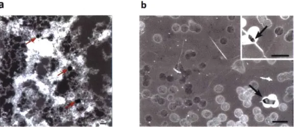
2.2. Two types of defects in graphene. (a) Intrinsic defects in graphene imaged by

STEM medium-angle annular dark field (MAADF). Scale bar is 10 nm. (b)

Fabrication tears in graphene imaged by high resolution SEM. Scale bars are 500 nm. Reprinted with permission from O'Hern et al. [7] Copyright 2012 American C hem ical Society. ... 2 1

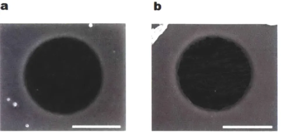
2.3. SEM images graphene transferred to TEM grids (a) without hafnia deposition and (b) with 40 cycles of hafnia deposition. Scale bars are 1 m... 23

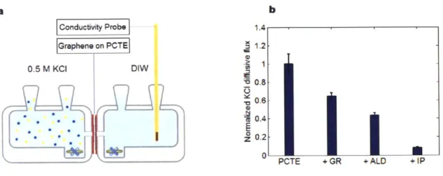
2.4. (a) Experimental setup for KCl diffusive leakage across the membranes. (b) KCl diffusive flux across the membrane after each fabrication and defect sealing step normalized by the flux through a bare PCTE membrane... 25

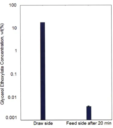
3.1. The concentration of glycerol ethoxylate of the draw solution (prepared as 10.66 wt%) and the feed solution after 20 min of water flux measurements. Reprinted with permission from O'Hern et al. [6] Copyright 2015 American Chemical S o ciety ... 3 2

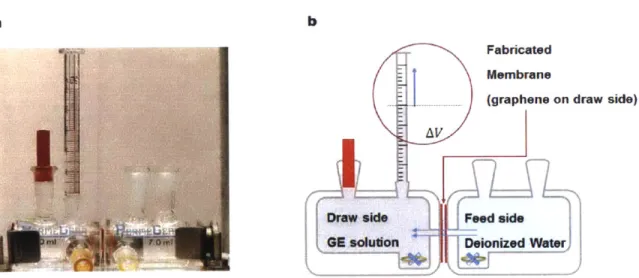
3.2. Experimental setup for forward osmosis driven water flux measurement experiment. (a) Customized 7.0 mL Side-Bi-Side glass diffusion cell (Permegear, Inc.) with 5.5 mm orifices and (b) its cross-sectional schematic. ... 34

3.3. Concentration polarization experienced by glycerol ethoxylate at the interface of graphene. (a) Draw solution is introduced to the graphene side and the glycerol ethoxylate concentration at the interface is comparable to the bulk concentration.

(b) Draw solution is introduced to the PCTE side and the glycerol ethoxylate

concentration at the interface is lower than the bulk concentration. (c) Measured water flux across the membrane when the draw solution is placed at the graphene side and the PC TE side. ... 37

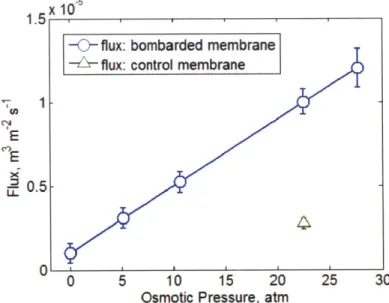
3.4. Calculated water flux across the graphene membrane against the corresponding osm otic pressure gradient... 39

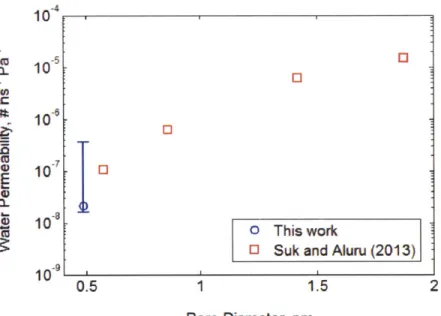
3.5. Experimental water permeability per single graphene pore and theoretical water permeability per pore from molecular dynamics simulation by Suk et al. [6,

2 3 ] ... 4 3

4.1. Calibration of conductivity probe against NaCl and MgSO4. (a) Measured conductivity against corresponding concentration of NaCl solution. (b) Measured conductivity against corresponding concentration of MgSO4 solution... 49

4.2. Experimental setup for osmotically driven ion and molecule transport measurement experiment. (a) Customized 7.0 mL Side-Bi-Side glass diffusion cell filled with AR solution at the graphene side. A fiber optic dip probe of UV-Vis spectrophotometer is placed at the draw solution side. (b) Cross-sectional schematic of AR transport measurement. ... 52

4.3. (a) Experimental and theoretical molar flux of NaCl, MgSO4, AR and TMRD driven by osmotic pressure gradient of 20 atm. (b) Experimental and theoretical rejection of NaCl, MgSO4, AR and TMRD exhibited by the graphene membrane.

List of Tables

3.1. Table 3. 1. Measured osmolality and target and measured osmotic pressure of glycerol ethoxylate solution of different concentration. ... 30

4.1. Conductivity probe and UV-Vis probe calibration coefficients for NaCl, MgSO4, A R or T M R D . ... 49

Chapter 1

Introduction

1.1 Motivation

Graphene is a single layer of sp2 _{bonded carbon atoms arranged in a hexagonal}

lattice. In its pristine state, monolayer graphene is reported to be impermeable to molecules even as small as helium. [1] Relying on electron beam nanosculpting, Fischbein et al. were able to introduce stable, controllable pores at nanometer-scale to multi-layered graphene. [2] Its atomic thickness (-0.34 A) and unparalleled ultimate tensile strength amounting to 130 GPa appoint graphene as a qualified candidate for high flux separation membrane withstanding high pressure. [3, 4] Due to the aforementioned remarkable characteristics, graphene had emerged as a next generation water purification membrane. Cohen-Tanugi et al. used molecular dynamics simulation to predict the water permeability through a single-layer graphene to be orders of magnitude higher than that exhibited by conventional reverse osmosis membranes. [5]

Although graphene has been drawing attention as a promising material for water purification membranes, most of the studies have been confined to theoretical investigation on it. Due to some challenges in membrane fabrication and transport measurements, only a few work has explored the idea of water purification membrane using graphene with experiments. In order for water purification membrane to be practically feasible, it not only requires high water flux across it,

but it also has to be highly selective to water, preventing the transport of ions and molecules. The primary impediment to its realization arises from the difficulty of fabricating large area graphene membrane free of defects and tears. Transferring single-layer graphene grown on copper catalyst substrate to other support membranes does not flawlessly translate the inherent impermeability of graphene, but results in 100-1000 nm scale tears from membrane handling. Graphene also

contains intrinsically present nanometer-scale (- 1-15 nm) defects and grain

boundaries arising from CVD synthesis process. Large area graphene composite membranes inevitably retain these intrinsic defects and fabrication tears, which allow for diffusive leakage of ions and molecules and sacrifice selectivity. In order for water purification membrane to exhibit high water permeability, water should be convectively driven by pressure gradient imposed across the graphene membrane. However, complexity in design consideration for convection-driven flow measurement has prevented the experimental attempts to employ graphene membranes in transport studies. Developing repeatable and reliable methods to drive water and molecules across graphene will be essential in characterizing the transport phenomena that have been only explored in theoretical regime.

1.2 Scope of Work

To take the preceding transport studies across graphene one step further, evaluation of graphene's potential as the backbone material for water purification and nanofiltration membranes should be accompanied by reliable methodologies to measure convective transport of water and molecules. The objective of this thesis is to osmotically drive water and ions/molecules in aqueous phase across graphene

membrane and compares the measured flux to the results from molecular dynamics simulation. Chapter 4 illustrates experimental design to measure convection dominated transport of salts and organic molecules of different sizes and discusses rejection performance of the defect tolerant graphene membrane. Chapter 5

summarizes the important findings and contributions of the thesis and discusses future work and direction.

Chapter 2

Fabrication of Large Area Defect Tolerant

Graphene Membranei

2.1 Single-Layer CVD Graphene Transfer to Porous PCTE

Membranes

To harness inherent impermeability and atomic thickness of graphene for water purification or nanofiltration purpose, it needs to be transferred to a porous substrate which serves as a mechanical support. Graphene transfer process developed by O'Hern et al. was followed and slightly modified to isolate ~ 1 cm2 _{monolayer CVD} grown graphene from copper foil and transfer it to a porous polycarbonate track etch

(PCTE) membrane with 200 nm pores. [7]

Throughout entire measurements and studies in this work, graphene composite membrane was fabricated with monolayer graphene synthesized on copper foil (JX Nippon Mining & Metals HA Foil) by Song et al. using low pressure

CVD process. After annealing the copper foil for 30 min in 1 000C H2 environment,

H2 and CH4 flow rates were set at 70 and 0.5 sccm, respectively, to synthesize

graphene on it for 30 min with the chamber pressure of 1.90 Torr.

In order to measure water and molecular transport across the synthesized monolayer graphene, it needs to be transferred from the copper foil to a porous

'In collaboration with Sean O'Hern, Yi Song, and Jing Kong, MIT. This works was published in Ref [6].

polymer substrate which provides mechanical integrity to the resulting composite membrane. Graphene transfer methods developed by O'Hern et al. exploiting solid-solid surface adhesion between graphene and a polymer substrate were adopted to minimize the adsorbing contaminates which are common byproducts of polymer sacrificial transfer methods. [7, 8, 9]

Polycarbonate track etch (PCTE) membranes from Sterlitech were used as porous target substrates for transfer. 200 nm pore fraction was 0.1 relative to the entire area and the surface of PCTE was free of PVP coating to ensure hydrophobicity. The synthesized monolayer graphene on copper foil was cut into a smaller piece (~ 5 mm x 5 mm) and was floated on a bath of APS-100 etchant

(ammonium persulfate, Transene) for 7 min to remove the backside graphene. Then, it was rinsed in two baths of deionized water (DIW) for 10 min each and air dried. To further enhance hydrophobicity, the PCTE membrane was immersed in 50 mmol didecylamine (Sigma-Aldrich) in ethanol for 1 h and rinsed in three subsequent baths of ethanol for 20 min each. An empty glass slide was covered with a weighing paper on which the back-etched copper piece was placed. Then, it was topped by the surface treated PCTE membrane with the centers aligned and the entire stack was covered by another glass slide. A round pipette tube was rolled over the top glass slide with light finger pressure to have the pliable PCTE membrane conform to the copper foil, enhancing a contact between graphene and PCTE. The resulting graphene-PCTE composite membrane sitting on the copper foil was floated on an

APS-100 bath and etched for 1.5 h in nitrogen chamber under 7 psi. After etching,

the membrane was rinsed by floating it on seven subsequent baths of DIW for 5 min each and immersing it in 50% ethanol/DIW and then air dried. The schematic of each step is illustrated in Figure 2.1.

Graphene Copper Graphene

*

Figure 2. 1. Entire process of single-layer graphene transfer to and PCTE didecylamine treatment.

2.2

Sealing Defects and Tears in Graphene

2.2.1 Intrinsic Defects and Fabrication Tears in Transferred Graphene

Ideally pristine graphene is atomically thin carbon lattice impermeable to the smallest molecules such as helium. [1] If the size of pores introduced to the pristine graphene could be controlled to be confined in an appropriate range, passage and blockage of ions/molecules following the steric exclusion would become feasible and the nanoporous graphene would serve as a reliable platform for a range of application including desalination, nanofiltartion and water purification. Nevertheless, the presence of intrinsic defects and fabrication tears allows for the diffusive transport of undesired ions and molecules, resulting in graphene composite membrane vulnerable to diffusive leakage of solutes. [7] When driving water and molecular transport across the nanoporous graphene under convection, a 10-fold increase in the effective diameter of a defect leads to a 1000-fold rise in permeation

FA]

Glass slide

PCTE

Graphene

of a solute through it. [10] Therefore, intrinsic defects on different length scales and tears from membrane fabrication should be eliminated, or at least minimized, to drive water transport across created sub-nano pores under convection, while blocking the passage of solutes of larger diameters.

Large area graphene synthesis following CVD process entails the formation of intrinsic defects during the growth. Impurities on copper foil or uneven growth over the entire surface may lead to nanometer-scale graphene defects including pinhole defects, single or multiple atomic vacancies, or grain boundaries. O'Hem at al. imaged the intrinsic defects in transferred monolayer graphene suspended on a TEM grid. [7] (See Figure 2.2) It was discovered that the transferred graphene contained intrinsically present defects ranging in 1 - 15 nm in diameter,

corresponding to the distribution before transferring the graphene from the copper foil it was grown on. They also investigated the diffusive transports of ions and molecules of different diameters and diffusivities through these intrinsic defects. Comparison between the diffusive leakage of KCl through a bare PCTE membrane and a graphene composite membrane indicates that intrinsic defects, majority of which populating in 1 - 10 nm range, are responsible for allowing diffusive leakage

a

Figure 2. 2. Two types of defects in graphene. (a) Intrinsic defects in graphene imaged by STEM medium-angle annular dark field (MAADF). Scale bar is 10 nm.

(b) Fabrication tears in graphene imaged by high resolution SEM. Scale bars are 500 nm. Reprinted with permission from O'Hern et al. [7] Copyright 2012

American Chemical Society.

Fabrication tears are defects on graphene incurred during the transfer, including handling, pressing and etching when outgassing APS-100 cannot escape the graphene surface and ruptures the carbon lattice. [7] They usually are on a larger scale of about 100 - 200 nm when compared to the intrinsic defects. (See Figure 2.2) A single defect in graphene only needs to be ~ 1.2 nm in diameter to have the same diffusive transport resistance as a single 200 nm PCTE pore. [10] Since the fabrication tears are generally two order of magnitudes greater in size than nanoscale intrinsic defects, the transport resistance diminishes by - 1 04-fold and the

graphene is virtually transparent to the diffusive transport. Thus, a few large tears suffice to allow for significant diffusive leakage of solutes across the graphene membrane, sacrificing its nanofiltration capability.

2.2.2 Sealing Intrinsic Defects - Atomic Layer Deposition

Intrinsic defects were covered by depositing metal oxides on the graphene composite membrane through atomic layer deposition (ALD). Metallic precursors in vapor phase are exposed to and deposited on a substrate at elevated temperature over cycles in a vacuum chamber. Defect regions in graphene have relatively higher surface energy due to their unsaturated carbon bonds than the pristine area. Thus, the metallic precursors are preferentially adsorbed to the intrinsic defect sites, while the most of the basal plane remain intact. [11, 12] Cambridge Nanotech Savannah Atomic Layer Deposition at the Center for Nanoscale Systems at Harvard University was used to perform atomic layer deposition on the graphene PCTE composite membrane. Hafnia was chosen as precursor gas due to its stability in water, while other available metallic oxides such as aluminum oxides might undergo change in composition or dissolve in water. After running 20 pre-cycles of hafnia without the graphene membrane inside the chamber to purge any impurities, a 40 min nitrogen purging was performed with the membrane inside, which was followed

by 40 cycles of hafnia at 130'C, ~ 400 mTorr. Ellipsometry on a silicon wafer which

underwent the identical procedure in the same chamber indicated that ~ 3.5 nm thick hafnia layer had been deposited on the graphene. After the hafnia deposition, SEM images of the graphene membrane suspended on TEM grids suggested that ~ 45.6%

of the entire area remained intact without dendritic oxides and could be available for the transport of water and solutes. [6] (Figure 2.3)

a

b

Figure 2. 3. SEM images graphene transferred to TEM grids (a) without hafnia deposition and (b) with 40 cycles of hafnia deposition. Scale bars are 1

sm.

2.2.3 Mitigating Fabrication Tears - Interfacial Polymerization

Since fabrication tears from membrane handling are generally at larger length scales than intrinsic defects, they cannot be sufficiently covered with hafnia through atomic layer deposition process. Instead of directly sealing the tears with precursors or nanoscale particles, an alternative method was sought to plug up the PCTE pores behind the graphene area with large tears. A process called interfacial polymerization was adopted and slightly adopted, where two reactive monomers are brought into contact at the interface between two immiscible solvents and react in the organic phase side to polymerize. [6, 13, 14]

In our process, the monomers were hexamethylenediamine (HMDA, Sigma-Aldrich) and adipoyl chloride (APC, Sigma-Sigma-Aldrich) which react to form nylon 6,6 precipitates. 5 mg/mL HMDA in water, with the pH adjusted to 9 by sodium bicarbonate, and 5 mg/mL APC in hexane were prepared. After filling the bottom reservoir of a 5.0 mL Franz cell (Permegear, Inc.) with the HMDA solution, a graphene-PCTE membrane after 40 cycles of hafnia deposition was placed with the graphene side down so that it could be in contact with the solution below. Then, the top cell was placed on the membrane and clamped, after which the APC solution was carefully introduced to the exposed PCTE side. After sealing the entire cell, the

reaction took place for 1 h and HMDA solution was replenished when its meniscus level dropped from evaporation. During the reaction, HMDA diffuses across the liquid-liquid interface to the organic phase side only where there are permeable

defects and tears in graphene. HMDA reacts with APC to form nylon 6,6 precipitates, impermeable polymer plugging the PCTE pores behind large enough tears through polycondensation. [13] Then, the top cell was consecutively rinsed with hexane and then with ethanol by carefully adding and removing with a pipette. As a last step, the cell was disassembled and the membrane was rinsed in three subsequent baths of ethanol and air dried. Confocal fluorescence microscopy imaging of the graphene membrane after interfacial polymerization verified that fluorescently labeled nylon 6,6 plugs are formed inside the PCTE pores behind the larger cracks and tears in graphene. Further details are slightly beyond the scope of this thesis and are discussed in our recent publication. [6]

2.2.4 Reduction in Diffusive Leakage across Graphene Membrane after Sealing Defects and Tears

Diffusive transport of KCl across the membrane was measured at each step of membrane fabrication and defect sealing process to estimate how much of the defects on different scales was mitigated following atomic layer deposition and interfacial polymerization. A membrane of interest was supported by adhesive silicone sheets (Grace Bio-Labs) on both sides and mounted on the Side-Bi-Side glass diffusion cell (Permegear, Inc.) with a 5.5 mm orifice. (Figure 2.4) The reservoir on the graphene side was filled with 0.5 M KCl (Sigma-Aldrich) solution, while the polycarbonate side reservoir contained degassed deionized water. Teflon

increase in conductivity of deionized water side of the cell which was captured every

15 s for 15 min by a Miniature Dip-In Conductivity Electrode (eDAQ, ET 915).

a b Conductivity Probe Graphene on PCTE 0.5 M KCI DIW 7) 7

i

Figure 2. 4. (a) Experimental setup for KCl diffusive leakage across the membranes.

(b) KCl diffusive flux across the membrane after each fabrication and defect sealing

step normalized by the flux through a bare PCTE membrane.

The slope of the measured conductivity values as a function of time was approximated and the system was assumed to reach a steady state in the first ten minutes, which led us to retrieve the linear data from the last five minutes. Relying on the relationship between the conductivity and the concentration of solution acquired from calibration, the calculated conductivity change rate was converted to the KCl molar flux across the membrane. After transferring a single-layer CVD graphene to a PCTE support, the KCl diffusive leakage reduced to ~ 65% that of bare PCTE. (Figure 2.4) Since the transferred graphene membrane contains intrinsic

defects and fabrication tears, it could not perform as an immaculate barrier to KCl transport, but allowed for diffusive leakage. Covering the intrinsic defects in transferred graphene with hafnia through atomic layer deposition brought the KCI leakage down to ~ 40%. Subsequent plugging of large fabrication tears with nylon

indicating that the two-step defect sealing process could mitigate - 88% of

potassium chloride diffusive leakage past defects and tears in graphene. Some permeable defects that are too large to be covered with hafnia or not completely plugged by nylon film could account for residual leakage after atomic layer

Chapter 3

Experimental Design and Measurement of

Osmotically Driven Water Flux

3.1 Experimental Design

3.1.1 Introduction of Subnanometer Pores to Defect Tolerant Graphene

Membrane'

After transferring large area single-layer graphene to a porous PCTE support and sealing defects at different length scales following the methods described in Chapter 2, high density of pores with controlled, narrow size distribution were introduced for the membrane to be highly permeable and selective to water. O'Hern et al. reported that irradiating single-layer graphene suspended on a holey-carbon TEM grid with gallium ions nucleates defects sites, which undergo rapid growth from potassium permanganate etching and grow into water permeable pores with a mean diameter ~ 0.4 nm. [10] The same procedure was followed in this work with the bombardment parameters modified to create single vacancy defects with a tighter size distribution so that we could ensure that transport or filtration across the

using FEI Helios NanoLabTM 600 DualBeam. [15, 16] Gallium ion beam with high

tension voltage of 1 kV and current of 6.9 nA was used to bombard the graphene membrane at an incident angle of 0'. At the dwell time of 3 ps/pixel, Ga+ ion beam scanning was performed at the resolution of 4096 x 3536 over 2.544 mm2 _{per shot.} This corresponded to ~ 1.87 x 1012 bombardment per each scanned area, or the bombardment density of ~ 7.32 x 1013 CM2_{. Then, the introduced reactive defect} sites were grown larger into permeable pores by exposing the bombarded graphene to 1.875 mM potassium permanganate etchant in 6.25% sulfuric acid for 1 h. [6, 17,

18] After mounting the bombarded graphene membrane on the diffusion cell, the

reservoir on the graphene side was filled with the acidic potassium permanganate solution and the opposite side was filled with deionized water. Teflon coated magnetic stir bars kept stirring both sides for 1 h throughout the oxidative etching process and the deionized water was removed and replenished every 15 min. When the etching was finished, each side of the cell was thoroughly rinsed with degassed deionized water for 5 times to remove any residual etchant in the cell.

3.1.2 Water Flux Driven by Forward Osmosis

Two-step defect sealing process described in Chapter 2 followed by ion bombardment and oxidative etching allows for the measurement and investigation of convectively driven water flux across nanoporous graphene membrane. Pore size distribution estimated from subtracting the carbon van der Waals radius subtracted from the center-to-center diameter resulted in a lognormal distribution with a mean diameter of ~ 0.162 nm. [6] Assuming that the van der Waals diameter of a water molecule is 0.275 nm, larger pores of a density ~ 1.57x 1012 cm-2 _{were expected to} be permeable to water, preventing the transport of ions and molecules, most of which are at least larger than 0.6 nm.

Taking advantage of the introduced subnanometer pores with narrow size distribution, osmotic pressure gradient was imposed to convectively drive water

across the nanoporous graphene membrane. The osmotic agent of choice was 98% glycerol ethoxylate (Sigma-Aldrich) with average molecular weight of ~1 kDa. Glycerol ethoxylate solution of weight percentage wt% was prepared in degassed deionized water to achieve target osmotic pressure according to the following relation [19]

logAwr = 4.87 + 0.8 (wt%)0 _.3 4 _(3.1)

where ziw denotes osmotic pressure (dyne/cm2_{) of the solution. The target osmotic}

pressure values of the glycerol ethoxylate solution used for water flux measurements were calculated according to the above equation and are listed in Table 3.1. The actual osmotic pressure was measured using osmometer and its procedure is discussed in Section 3.1.3.

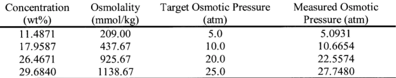
Table 3. 1. Measured osmolality and target and measured osmotic pressure of glycerol ethoxylate solution of different concentration.

Concentration Osmolality Target Osmotic Pressure Measured Osmotic

(wt%) (mmol/kg) (atm) Pressure (atm)

11.4871 209.00 5.0 5.0931

17.9587 437.67 10.0 10.6654

26.4671 925.67 20.0 22.5574

29.6840 1138.67 25.0 27.7480

Imposing osmotic pressure gradient is not the only method to drive water flux across the nanoporous graphene membrane. Introducing a difference between the liquid levels of each fluid reservoir across the membrane, one could build a hydrostatic head to convectively drive water. However, forward osmosis driven flow was adopted in this studies due to its several advantages that make water flux measurement across graphene more accurate and reliable.

is also preferable in that it remains nearly constant over the course of water flux experiment. The gradient across the graphene membrane can vary in two possible situations: 1) dilution of the draw (glycerol ethoxylate) solution by incoming water flux or 2) diffusive leakage of draw solutes across the membrane. With the current measurement setup, the original volume of the draw solution (mL scale) is approximately three orders of magnitudes greater than that of water (tL scale) driven across them membrane over 20 min. Thus, the concentration (weight percentage) of the draw solutes in solution is barely affected by dilution over the course of measurement. Two-step defect sealing process described in Section 2.2 significantly reduces the number of intrinsic defects and fabrication tears, both of which could be potential diffusive pathways for glycerol ethoxylate molecules. Furthermore, majority of the permeable pores in graphene introduced by gallium ion bombardment and potassium permanganate etching are expected to sterically hinder the diffusion of the draw solutes. [6, 10] When the draw solution concentration was 10.66 wt% (corresponding to the target osmotic pressure of 10 atm), UV-vis absorbance measurement revealed that the concentration of glycerol ethoxylate in the feed side (filled with degassed deionized water) after 20 min of forward osmosis was less than 0.01 wt%, indicating that a negligible amount of the draw solute diffused across the graphene membrane. (See Figure 3.1.)

For hydrostatic pressure driven flow, water transport would bypass smaller pores and preferentially take place through larger pores. Assuming that a graphene pore is a channel of finite length and diameter with circular-section, its hydrodynamic resistance scales inversely proportional to the third-order of its diameter. [7] Therefore, a pore twice larger in size has theoretically ~ 8-fold lower convective transport resistance and thus permits a little less than an order of magnitude higher water flux. Thus, convectively driven water transport could be dominant not through created subnanometer pores, but across the remaining permeable graphene defects that are either too large to be covered by hafnia or too small to be sealed by nylon 6,6 film. However, osmotically driven water transport

is feasible only through pores smaller than the size of glycerol ethoxylate molecules, since larger pores would not even establish osmotic pressure gradient, which relies on the semipermeability of the membrane. Water flux measurements from forward osmosis could give us a better estimate of transport across smaller pores created by gallium ion bombardment and oxidative etching.

100 0 0 C 10 1 0.1 0.01 0.001

Draw side Feed side after 20 min

Figure 3. 1. The concentration of glycerol ethoxylate of the draw solution (prepared as 10.66 wt%) and the feed solution after 20 min of water flux measurements. Reprinted with permission from O'Hern et al. [6] Copyright 2015 American Chemical Society.

adjusted to match the measured value to 290 mmol/kg by shifting the entire calibration curve by the same amount for offset calibration. As a second step, the measuring disc was removed and 10 [tL of 1000 mmol/kg standard was dropped on a new disc. The measured value was looked up in calibration monograph provided in the user manual to obtain a corresponding set value. Then, as gain calibration, the

1000 control was adjusted until the set value was reached by changing the slope of

the calibration curve, affecting all the values proportionately. Both offset calibration and gain calibration were repeated until the measured values agreed with 290 mmol/kg and 1000 mmol/kg, respectively.

After calibrating the osmometer, the osmolality value of the each glycerol ethoxylate solution used for water flux measurement was measured in triplicate. According to the Van't Hoff equation, the glycerol ethoxylate solution of osmolality m (mol/kg) can impose osmotic pressure gradient 4w (atm) as follows [20],

A7 = RTv Pwater m (3.2)

where R denotes the universal gas constant (8.205 X 10- m3 atm / K*mol ), T is temperature, v is Van't Hoff coefficient, and Pwater is density of water. The measured osmolality and corresponding osmotic pressure values are listed in Table 3.1 in Section 3.1.2 and the theoretical and measured values show reasonable agreement with each other.

3.1.4 Experimental Setup and Measurement

Water transport driven by osmotic pressure gradient was performed in a custom designed 7.0 mL Side-Bi-Side glass diffusion cell (Permegear, Inc.) with 5.5 mm orifices. It is a scaled-up version of the diffusion cell used for the KCl diffusive transport measurement (Figure 2.2), but one of the open ports of the cell was connected to a 250 pL graduated syringe (Hamilton Gastight 1725) for water transport measurement and sealed with wax for leakproof connection. (Figure 3.2)

The defect tolerant graphene membrane with created subnanometer pores was mounted on the cell so that it faced towards the syringe side, following the same procedure described in Section 2.2.4. After tightly clamping the cell together, 90% ethanol in water was introduced to both sides of the cell to wet the membrane before measurement, followed by 5 rounds of rinsing with degassed deionized water for 2 min each.

ab

Fabricated Membrane

I

Draws~deFoed side GE soluton Deionized Water

Figure 3. 2. Experimental setup for forward osmosis driven water flux measurement experiment. (a) Customized 7.0 mL Side-Bi-Side glass diffusion cell (Permegear, Inc.) with 5.5 mm orifices and (b) its cross-sectional schematic.

Membrane wetting and rinsing were followed by preparing draw (glycerol ethoxylate) solution of specified concentration: 11.49, 17.96, 26.47, and 29.68 wt% corresponding to osmotic pressure of 5, 10, 20, and 25 atm, respectively. 7.4 mL of the draw solution was slowly pipetted to the graphene side (draw side) of the diffusion cell where the graduated syringe stood and 7.25 mL of degassed deionized water was introduced to the syringe-less side (feed side), making sure that no

coated magnetic stir bars kept vigorously stirring each solution to minimize the effects of concentration polarization. The rise of the liquid meniscus level along the syringe resulting from the incoming water flux to the draw side was periodically monitored by a digital camera every minute. Each water flux measurement was performed three times for 20 min each by replenishing with new solution to capture the uncertainties from measurement or concentration of the draw solution.

Internal Concentration Polarization

While the single-layer graphene is atomically thin, the porous PCTE support membrane is of finite thickness of 10 tm and thus water flux across the

graphene-PCTE membrane is subject to external and internal concentration polarization. Gray

et al. investigated internal concentration polarization in forward osmosis

measurement and reported that it could either minimal or severe depending on the orientation of the membrane. [21] Forward osmosis membranes are composed of two components - an active layer where the transport across the interface occurs and a (porous) support layer which gives mechanical stability and is usually thicker. The driving force of forward osmosis is the effective osmotic pressure gradient across the active layer, which takes the advantage of the semipermeability of the membrane.

If the draw solution were placed on the support layer side, the draw solutes

have to diffuse through the pores of the support layer to the interface. Since the diffusivity of the draw solutes is likely to be low due to their large size, the concentration inside the pores, Cpore, tends to decrease as a function of the distance they travel. Therefore, at the far end of the pores, the Cpore could be considerably lower than the concentration of the bulk draw solution, Cboik. Furthermore, the influx

of osmotically driven feed solution to the draw solution side displaces the draw solutes further away from the active layer, a phenomenon defined as dilutive internal concentration polarization. [21, 22] Therefore, a large fraction of the original

driving force could be consumed by external and internal concentration polarization and the flux of feed solution could be reduced.

On the other hand, if the draw solution is introduced to the active layer side, the distance the solute needs to diffuse to reach the interface could be significantly reduced by order of magnitude. Thus, concentration inside the active layer pores

Cpore would not experience as severe reduction and Cpore at the interface between the

draw and the feed solution could be comparable to Cbulk. Then, a great portion of the original driving force could remain undiminished, resulting in a higher net osmotic pressure gradient across the membrane.

In our case, the active layer was graphene of subnanometer thickness and the support layer was a porous PCTE membrane with 10 pm thickness. The thickness differs by more than five orders of magnitude and the orientation of the membrane could be essential in reducing the effects of internal concentration polarization. Figure 3.3 (a) and (b) illustrate the expected glycerol ethoxylate concentration profile depending on whether the draw solution was introduced to the graphene side or the PCTE side. Then, the water flux measurement was measured with two opposite membrane orientations by switching the side the draw solution was introduced to. (Figure 3.3 (c)) Although there was not a large difference in the water flux of each orientation, placing the draw solution in contact with the graphene layer resulted in higher water flux. Considering that ~ 10% of flux from the draw solution at the PCTE side case might have been partially assisted by the pressure gradient from the hydrostatic head in the graduated syringe, the water flux difference between the two orientations could be as high as 20%. Therefore, throughout the water flux measurement experiment, the draw solution was always introduced to the graphene side reservoir.

Draw Solution Feed Solution C

___ ___ ___x 1 ~

Flow dii ction

c - - - 1.2

cpc,

CPCII

E0.8

b

Feed Solution Draw Solution 2 0.6

Flow d re tion 0.4

. . . 0.2

cpOe

0 Graphene side PCTE side

10 pm _,

Figure 3. 3. Concentration polarization experienced by glycerol ethoxylate at the interface of graphene. (a) Draw solution is introduced to the graphene side and the glycerol ethoxylate concentration at the interface is comparable to the bulk concentration. (b) Draw solution is introduced to the PCTE side and the glycerol ethoxylate concentration at the interface is lower than the bulk concentration. (c) Measured water flux across the membrane when the draw solution is placed at the graphene side and the PCTE side.

3.2 Experimental Measurement of Water Permeability of

Graphene

3.2.1 Calculation of Experimental Water Permeability

After forward osmosis water transport measurement was performed, water permeability of graphene membrane at different conditions was calculated. Using

the Multi-point Tool in ImageJ, the rise in draw side meniscus level along the graduated syringe during 20 min was captured and converted into volume of water transported across the graphene membrane. The measured water flux jmeasured and permeability Kmeasured were calculated according to the following definition:

rm AV Imeasured

[]

[rm

where A V is the volume of water transported across the membrane, d is the diameter of the cell orifice (5.5 mn), Acorrection is the area matching factor of the two orifices

(0.76), y is the PCTE membrane porosity (0.1), At is the time for each measurement (1200 s), and A4f is the osmotic pressure gradient across the membrane (5 -25 atm).

The calculated water flux is plotted against the corresponding osmotic pressure gradient in Figure 3.4.

As discussed in Section 3.1.2, the created subnanometer pores are not the sole transport pathways for water flux. Uncovered residual defects and nylon 6,6 plugs that are partially formed or damaged by oxidative etching could also allow for osmotically driven water flux. Therefore, the measured water permeability Kmeasured

is comprised of two contributions, one from the created subnanometer pores and the other from the defects or the nylon film:

Kmeasured ~ Kpores + Kdefects (3.5)

To estimate to what extent the intrinsic defects and the nylon film are contributing to the measured water flux, a control membrane was prepared without introducing the pores with gallium ion bombardment. After the graphene transfer,

one, the control membrane, was not bombarded. After mounting the control membrane on the measurement cell, 1 h of potassium permanganate etching followed. Water transport across the control membrane is now not through the created pores, but through intrinsic defects and nylon plugs. (See Figure 3.4) A discrepancy between the water flux between the bombarded and control membranes at osmotic pressure of 22.56 atm indicates that osmosis driven water flux was predominantly through the created subnanometer pores.

1.5

-0- flux: bombarded membrane

- flux: control membrane 1 E E 0.5 4 0 5 10 15 20 25 30

Osmotic Pressure, atm

Figure 3. 4. Calculated water flux across the graphene membrane against the corresponding osmotic pressure gradient.

Then, water permeability across the control membrane (Kdefects = 1.7823 x 10-12 m/Pa-s at 22.56 atm) can be subtracted from the measured permeability

(Kmeasured = 4.3751 x 10-12 m/Pa-s) across the bombarded membrane to account for

the water transport across the created pores only (Kpores = 2.5927 x 10-12 m/Pa-s). To

evaluate the water permeability of the graphene pores, the uncovered graphene area available for transport should be taken into account instead of the entire graphene membrane area as in Equation 3.4. Therefore, the subtracted water permeability was divided by the portion of the graphene not covered by hafnia nor by nylon 6,6 film:

K Kpores

Kgraphene = P (fi (3.6)

OALD OIP

where PALD denotes the fraction of graphene not covered by hafnia and Pwj denotes the fraction of PCTE pores not sealed by nylon 6,6 plugs. Confocal fluorescence microscopy and Scanning Electron Microscopy imaging analysis revealed that

-45.6% of graphene and -93.3% of PCTE pores were available for transport. [6] The resulting water permeability Kgraphene through graphene area available for transport was approximately 6.6640 x 10" m/Pa-s and will be discussed further in the next

section for permeability per single graphene pore.

3.2.2 Calculation of Uncertainties in Experimental Water Permeability

After calculating the water flux and permeability across the graphene, uncertainties in these extracted values were estimated following the standard propagation of error formula:

SG = ) X (3.7)

where G = G(xi) denotes either flux or permeability as a function of a variable xi and ix denotes the uncertainty in the variable.

Uncertainties can arise from several different sources including the osmotic pressure gradient imposed by initial concentration of the draw solution and the feed solution, the porosity of the PCTE membranes, and the volume of water transport driven across the membrane measured from the graduated syringe reading. All flux measurements were performed in triplicate to capture variability among different

including the osmotic pressure gradient and area of the membrane seen by the orifices were estimated to be within the 5% of the original predetermined values. Then, the uncertainty values were incorporated into Equation 3.7 and the uncertainties in extracted flux and permeability were evaluated by summing up the

contribution from each variable.

3.3 Estimation of Permeability of Single Graphene Pore'

3.3.1 Pore Size Distribution and Water Permeability per Single

Graphene Pore

Using molecular dynamics simulation, researchers have attempted to theoretically evaluate the water flux across a pore in monolayer graphene. [5, 23] For a comparison with the permeability foreseen by theories, experimental water permeability through a single graphene pore in our membrane had to be estimated. Analyzing the aberration corrected STEM images of graphene on TEM grids, size distribution of the water permeable pores was obtained. [6]

Although the STEM was capable of resolving the void space within the pristine hexagonal graphene lattice, it is too small to be considered a water permeable pore since it can prevent even helium from traveling across it. Pore size determined by open area from electron microscopy imaging is likely to be different from what molecules traveling across it might see. To better define the pore diameter, the convention suggested by Cohen-Tanugi and Grossman was adopted and slightly modified in this work. [5] They defined the pore as an open area not overlapped by carbon atoms simulated as van der Waals spheres and calculated the effective diameter of the pore as follows:

4 Area

deffective = (3.8)

In this work, the distance between the center of a carbon atom and the edge of its electron cloud was measured to be 0.065 nm, which was added to the effective pore radius to estimate a carbon center-to-center distance of a pore. Then, the van der Waals radius (0.17 nm) of a carbon atom was subtracted to obtain the adjusted effective diameter of a pore. Taking the size of a single water molecule into account, pores larger than 0.275 nm were considered permeable to water.

Analyzing the STEM images with polygon selection tool in ImageJ, adjusted effective diameters of the 156 pores were measured according to Equation 3.8 over

393.64 nm2 _{of graphene area and the density of pores greater than 0.275 nm was ~}

4.32 x 1012 cm2. Since the number of counted pores was not sufficiently high to

define the pore size distribution, a lognormal distribution was constructed using MATLAB based on the statistics from image analysis of the pores to simulate pores over 1 [tm2 _{of graphene area with the same pore density as measured one. From the}

reproduced lognormal curve, the density of the water permeable pores was approximately 1.59 x 1012 cm2, or ~ 6.6% of the entire pores. More discussion and

methods are elaborated in our recent publication. [6]

With the density of water permeable pores estimated, water permeability of a single graphene pore can be extracted from the permeability of graphene Kgraphene from the following equation:

Ksingie-pore Kgraphene Pwater 1

snIp Pa]r pore MWwater NA

agreement with prediction from molecular dynamics simulation by Suk et al. [6, 23] (See Figure 3.5) The consistency between the experimental values and theoretical calculation indicates that imposing osmotic pressure gradient across the membrane was an applicable method to measure and extract the high permeability of graphene to water flux. 10 -5 0 0- 10 10 0 7 10 0 0~ 10 _{0 This work}

0 Suk and Aluru (2013)

10-9

0.5 1 1.5 2

Pore Diameter, nm

Figure 3. 5. Experimental water permeability per single graphene pore and theoretical water permeability per pore from molecular dynamics simulation by Suk

et al. [6, 23]

3.3.2 Calculation of Uncertainties in Experimental Water Permeability The major sources of the error presented in the plot are primarily from the uncertainties in actual number of graphene pores permitting the water transport. They include the portion of the graphene free of hafnia deposition, the portion of

PCTE pores not blocked by nylon plugs, the pore density of graphene affected by

etching condition and contamination, and the inherent porosity of PCTE pores. Hafnia deposition has the greatest uncertainties since it may not be uniformly coating the entire graphene area, but dependent on the surface adsorbants

amount on graphene. The upper bound and lower bound for area fraction of graphene uncoated with hafnia were speculated at 0.75 and 0.20, respectively, to

account for its high uncertainty from the SEM image analysis. Confocal fluorescence microscopy confirmed the presence of nylon 6,6 plugs in PCTE pores and revealed that 93.3% of the entire pores remained unblocked. It was assumed that there was 3% variability, resulting in upper/lower bounds of 0.96 and 0.87,

respectively. The pore density estimated in Section 3.1.2 was based on the graphene on TEM grids which had been etched by floating the entire sample on the potassium permanganate surface. However, the graphene membrane used for water flux measurements was etched within the diffusion cell by introducing the etchant and deionized water to the graphene side and the opposite side, respectively, which could either double or halve the pore density acquired from one-sided etching. The role of surface contamination in preventing the transport still remains unexplored, and it was assumed that the adsorbed contaminants can lower down the effective pore density by three-fold. [6] The inherent porosity of PCTE membranes and its upper/lower bounds were provided by Sterlitech, which were 0.1 0.015.

Assuming that the major sources of uncertainties described above are all independent, the highest and lowest pore density could be estimated by multiplying the upper bounds and lower bounds, respectively, from each source. Then, the maximum/minimum estimation of the water permeability per pore could be acquired by reflecting this variability in total number of pores. Although it may be overestimating the actual deviation we might observe from measurements on every replicated membrane, the conservative approaches taken in estimation are expected to capture any variability arising from membrane fabrication and transport measurements.

Chapter 4

Experimental Design and Measurement of

Osmotically Driven Mass Transport

4.1 Experimental Design

4.1.1 Selection of Solutes

Measurements of water flux across the defect tolerant graphene membrane verified that the forward osmosis is a reliable method to drive water through subnanometer scale created pores in graphene. The measured permeability per single graphene pore was fairly consistent with the theory predicted by molecular dynamics simulations and confirmed the feasibility of graphene as a material for highly water permeable membranes. The next quest should be to explore the osmotically driven transport of ions and molecules across the graphene membrane and seek size selectivity.

Water soluble solutes of different sizes first needed to be selected to examine the size selective mass transport. For smaller, subnanometer solutes, sodium chloride (NaCl) and magnesium sulfate (MgSO4) were chosen. Since ions are solvated in an aqueous solution, their hydrated diameter should be taken into

for Mg' and S42- ions and the diffusivity was 0.788 x 10-9 m2/s. [24, 26] For

organic molecules beyond subnanometer scale, Allura Red AC (AR) and 4.4 kDa Tetramethylrhodamine isothiocyanate-Dextran (TMRD) were selected. The Stokes-Einstein hydrodynamic radius and diffusivity of Allura Red AC were estimated to be 0.5 nm and 0.36 x 10-9 m2/s by Werts et al. [27] 4.4 kDa Dextran,

the largest organic molecules tested, had the 1.86 nm of Stokes-Einstein radius and

0.138 x 10-9 m2_{/s diffusivity as reported by Kuz'mina et al. [28] Any larger solutes}

were not explored considering the size distribution of the introduced graphene pores.

4.1.2 Calibration of Conductivity Probe and UV-vis Spectroscopy Probe

Studying the transport of ion and molecules in aqueous phase requires precise measurements of the transport of solutes and solvent, which is degassed deionized water. The water transport across the graphene membrane was again measured by detecting the change in volume in the draw solution side, as described in Section 3.1.4, and the same strategy was adopted in mass transport studies. The osmotic pressure gradient across the membrane drove the feed solution, which was aqueous solution of ions or molecules, to the draw solution side. The transport of solutes resulted in the increase in concentration of the draw solution, whose rate could be converted to estimate the molar flux of solutes across the membrane. Directly comparing the initial and the final concentration of the draw solution falsely assumes that solute transport is a linear function of time throughout the measurement, which does not take into account the time to reach steady state. Therefore, in situ monitoring of concentration change would be desirable to measure the solute transport as a function of time.

Conductivity Probe Calibration against Salts

Concentration rise in the draw solution from osmotically driven salt transport is reflected in consequent increase in conductivity. As cations and anions travel across

the graphene membrane, conductivity of the draw solution increases proportionally to the total number of transported ions and its temporal change was detected by a conductivity probe. To figure out the proportionality between the concentration and conductivity, the conductivity had to be calibrated over a wide range of salt

concentration.

NaCl solution was prepared in five different concentrations, which were

0.001, 0.005, 0.01, 0.05 and 0.1 mM. Since the conductivity measurement in the

osmotically driven solute transport experiment was performed in the draw solution with 26.47 wt% of glycerol ethoxylate, the salt solution for calibration was also prepared in the glycerol solution of the same concentration. Then, each solution was filled into three separate centrifuge tubes and the conductivity was measured once in each tube in order of rising concentration with a Miniature Dip-In Conductivity Electrode (ET915, eDAQ). Then, the measurement was repeated in order of decreasing concentration, then again of increasing concentration to avoid introducing any bias to the conductivity probe. The entire procedure was repeated with MgSO4 in the exactly same manner.

The measured conductivity values were plotted against the corresponding salt concentration and linear regression was carried out to establish the 1 St order relationship as follows:

1

C = -- bo _(4.1)

where C is the molar concentration of each salt solution, - is the conductivity (mS/cm) and the bo and b1 are the calibration coefficients estimated by linear fitting

in MATLAB. The calibration curves for NaCl and MgSO4 are presented in Figure 4.1 and the calibration coefficients are summarized in Table 4.1.

x 10 x 10 8 2 8 E -- E E E 2.6 ~6 6- -0 0 4 4 4y =r 37.372 x + 0.0038 - ' * Y 57.149*x + 0.0033 *0 0.2 0.4 0.6 0.8 1 1.2 0 0.2 0.4 0.6 0.8 1 1.2 Concentration, M x 10, Concentration, M x 104

Figure 4. 1. Calibration of conductivity probe against NaCl and MgSO4. (a) Measured conductivity against corresponding concentration of NaCl solution. (b) Measured conductivity against corresponding concentration of MgSO4 solution.

Table 4. 1. Conductivity probe and UV-Vis probe calibration coefficients for NaCl,

MgSO4, AR or TMRD.

bo bi b2

NaCl 0.0038 mol l-' 37.372 mS-cm-'/mol-L-1 N/A

MgSO4 0.0033 molL-1' 57.149 mS-cm-I/moL-: N/A

AR 0.353 x 10-4 mol-L1 0.435 x 104 mo-L-1 0.00730 x 10~4 mol L-1

TMRD -3.112 x 10-4 mol L-' 4.517 x 10-4 mol-L-1 0.0705 x 10-4 mol-L-'

Conductivity Probe Calibration against Organic Molecules

Concentration rise in the draw solution from osmotically driven organic molecule transport is reflected in consequent increase in absorbance in UV-Vis (Ultraviolet-visible) spectroscopy. It uses a beam of light in the range of the ultraviolet and visible to transmit it through a sample in a transparent container. Different species absorb lights of different wavelengths and thus the acquired absorbance peak is characteristic to the tested species. According to the Beer-Lambert Law, the

b