An Analysis of Representations for Protein
Structure Prediction
by
Barbara K. Moore Bryant
S.B., S.M., Massachusetts Institute of Technology (1986)
Submitted to the Department of Electrical Engineering and
Computer Science
in partial fulfillment of the requirements for the degree of
Doctor of Philosophy
at the
MASSACHUSETTS INSTITUTE OF TECHNOLOGY
September 1994
( Massachusetts Institute of Technology 1994
Signature
of
Author
... ,... ...-..
..
Department of Electrical Engineering and Computer Science
September 2, 1994
Certified by... ...
.
--Patrick H. Winston
Professor, Electrical Engineering and Computer Science
This Supervisor
frtifioA
ho,Tomas o) no-Perez
and Computer Science
Thp.i. .,nPrvi.qnr
Accepted by
..
...
, a ,-
.
·
F'
drY
.../
Frederic R. Morgenthaler
~)Departmental /Committee on Graduate Students
%-"UL vL.Lv--k &y .
An Analysis of Representations for Protein Structure
Prediction
by
Barbara K. Moore Bryant
Submitted to the Department of Electrical Engineering and Computer Science on September 2, 1994, in partial fulfillment of the
requirements for the degree of Doctor of Philosophy
Abstract
Protein structure prediction is a grand challenge in' the fields of biology and computer science. Being able to quickly determine the structure of a protein from its amino acid sequence would be extremely useful to biologists interested in elucidating the mechanisms of life and finding ways to cure disease. In spite of a wealth of knowl-edge about proteins and their structure, the structure prediction problem has gone unsolved in the nearly forty years since the first determination of a protein structure by X-ray crystallography.
In this thesis, I discuss issues in the representation of protein structure and se-quence for algorithms which perform structure prediction. There is a tradeoff between the complexity of the representation and the accuracy to which we can determine the empirical parameters of the prediction algorithms. I am concerned here with method-ologies to help determine how to make these tradeoffs.
In the course of my exploration of several particular representation schemes, I find that there is a very strong correlation between amino acid type and the degree to which residues are exposed to the solvent that surrounds the protein. In addition to confirming current models of protein folding, this results suggests that solvent exposure should be an element of protein structure representation.
Thesis Supervisor: Patrick H. Winston
Title: Professor, Electrical Engineering and Computer Science Thesis Supervisor: Tomas Lozano-Perez
Title: Professor, Electrical Engineering and Computer Science
Acknowledgments
F'or their support, I thank my thesis committee, the members of the Artificial Intelli-gence Laboratory, Jonathan King's group, the biology reading group, Temple Smith's core modeling group at Boston University, NIH, my friends and family.
The following people are some of those who have provided support and encour-agement in many ways. To those who I've forgotten to list, my apologies, and thanks. Bill Bryant, Ljubomir Buturovic, John Canny, Peggy Carney, Kevin Cunningham, Sudeshna Das, Cass Downing-Bryant, Rich Ferrante, David Gifford, Lydia Gregoret, Eric Grimson, Nomi Harris, Roger Kautz, Jonathan King, Ross King, Tom Knight, Kimberle Koile, Rick Lathrop, Tomas Lozano-P6rez, Eric Martin, Mark Matthews, Michael de la Maza, Bettina McGimsey, Scott Minneman, Doug Moore, Jan Moore, Stan Moore, Ilya Muchnik, Raman Nambudripad, Sundar Narasimhan, Carl Pabo, Marilyn Pierce, Geoff Pingree, Tomaso Poggio, Ken Rice, Karen Sarachik, Richard Shapiro, Laurel Simmons, Temple Smith, D. Srikar Rao, Susan Symington, James Tate, Bruce Tidor, Bruce Tidor, Lisa Tucker-Kellogg, Paul Viola, Bruce Walton, Teresa Webster, Jeremy Wertheimer, Jim White, Patrick Winston, and Tau-Mu Yi.
Contents
1 Overview
1.1 Why predict protein structures? ... 1.2 Background ...
1.2.1 Secondary structure prediction .
1.2.2 Tertiary structure prediction . 1.3 My work .
1.3.1 Hydrophobic collapse vs. structure nucleation and 1.3.2 Modeling hydrophobic collapse.
1.3.3 Pairwise interactions: great expectations
1.3.4 Amphipathicity ... 1.4 Outline of thesis . . . . . .. . . . . . . . . . . . . . . . . . . . propagation . . . . . . . . . .. .. . . . . 2 Background 2.1 Knowledge representation.
2.1.1 Single residue attributes ... 2.1.2 Attributes of residue pairs ...
2.2 Contingency table analysis ... ... 2.2.1 Contingency tables.
2.2.2 Questions asked in contingency table analysis ... 2.2.3 Models of data ...
2.2.4 A simple contingency table example ... 2.2.5 Loglinear models ...
2.2.6 Margin counts .
2.2.7 Computing model parameters.
2.2.8 Examining conditional independence with loglinear models
2.2.9 2.2.10
Comparing association strengths of variables ... Examples of questions ... 3 Single-Residue Statistics 3.1 Introduction. 3.2 Method ... 3.2.1 Data . 3.2.2 Residue attributes . .
3.2.3 Contingency table analysis 3.3 Results and Discussion ...
15 15 20 23 25 30 31 32 33 34 34 35 35 36 39 39 40 40 41 42 47 48 49 49 49 52 54 54 54 54 55 55 56
...
...
...
...
...
...
3.3.1 Loglinear models. 3.3.2 Model hierarchies.
3.3.3 Nonspecific vs. specific amino acid representation 3.4 Conclusions ...
3.4.1 Solvent exposure is of primary importance .... 3.4.2 Grouping residues by hydrophobicity class ....
3.4.3 Attribute preferences ... . 4 Paired-Residue Statistics 4.1 Introduction. 4.2 Methods. 4.2.1 Data. 4.2.2 Representational attributes ...
4.3 Results and Discussion ... 4.3.1 Non-contacting pairs.
4.3.2 Contacting pairs; residues grouped into three classes . 4.3.3 Contacting residues: all twenty amino acids ... 4.4 Conclusions ...
5 Distinguishing Parallel from Antiparallel
5.1 Summary . . . .
5.2 Methods ...
5.2.1 Protein data ...
5.2.2 Definition of secondary structure, and topological relationships. 5.2.3 Counting and statistics ...
5.2.4 Contingency table analysis ... 5.3 Results and Discussion ...
5.3.1 Amino acid compositions of parallel and antiparallel beta
struc-ture.
5.3.2 Solvent exposure ... 5.3.3 Position in sheet ... 5.3.4 Grouping residues into classes 5.3.5 Contingency Table Analysis 5.4 Implications ...
5.4.1 Protein folding and structure 5.4.2 Secondary structure prediction . 5.4.3 Tertiary structure prediction
6 Pairwise Interactions in Beta Sheets
6.1 Introduction. 6.2 Method.
6.2.1 Significance testing ... 6.3 Results and Discussion ...
6.3.1 Counts and preferences ...
6.3.2 Significant specific "recognition" of beta pairs
. . . .... . . . 56 . . . .... . . . 59 . . . .... . . . 65 . . . .... . . . 71 . . . .... . . . 71 . . . .... . . . 71
...
72
73 73 74 74 74 76 76 81 85 87 89 . . 89 . . 91 . . 91 91 92 94 94 . . . 94 . . . .101 . . . 105 . . . 106 . . . 106 . . . ... . ... 111 . . . ... . ... .... 111 . . . ... . ... 111 . . . 112 113 . . . 113 . . . 114 . . . 115 . . . 115 . . . 115 .. .. . . . 1286.3.3 Significant nonspecific recognition ...
6.3.4 Solvent exposure ... . .
6.3.5 Five-dimensional contingency table .
6.3.6 Nonrandom association of exposure ... 6.3.7 Unexpected correlation in buried (i,j + 1) pairs.
6.4 Conclusions
...
.
7 Secondary Structure Prediction
7.1 Introduction.
7.2 Related Work ...
7.2.1 Hydrophobicity patterns in other secondary structure predic-tion methods ...
7.2.2 Neural Nets for Predicting Secondary Structure 7.2.3 Periodic features in sequences ...
7.3 A representation for hydrophobicity patterns ... 7.3.1 I, and I: maximum hydrophobic moments
7.3.2 Ch 7.3.3 De
aracterization of I, and I, ...
,cision rule based on I, and Io ... 7.4 Method ... 7.4.1 Neural network .... 7.4.2 Data ... 7.4.3 Output representation 7.4.4 Input representation 7.4.5 Network performance 7.4.6 Significance tests . . . 7.5 Results. ... 7.5.1 Performance. 7.5.2 Amphipathicity ....
7.5.3 Amino acid encoding 7.5.4 Learning Curves .... 7.5.5 ROC curves ... 7.5.6 Weights ... 7.6 Conclusion. ... 8 Threading 8.1 Introduction. 8.1.1 Threading algorithm.
8.1.2 Pseudopotentials for threading ... 8.1.3 Sample size problems ... 8.1.4 Structure representations.
8.1.5 Incorporating local sequence information 8.2 Method ... 8.2.1 Data. 8.2.2 Threading code ... 8.2.3 Structure representations ... 181 182 182 188 189 192 193 194 194 194 194 128 129 131 131 135 139 141 141 142 142 144 146 147 148 150 152 153 157 159 159 161 162 165 166 166 166 168 169 169 173 180 . . . .: : . . . .
...
...
...
...
...
...
...
...
...
S.2.4 Amino acid counts ...
$.2.5 Scores for threading; padding ... 8.2.6 Incorporating local sequence information. 8.3 Results and Discussion ...
$.3.1 Counts.
S.3.2 Likelihood ratios ... . .
8.3.3 Comparison of singleton pseudopotential components 8.3.4 Incorporating sequence window information ...
S.3.5 Splitting the beta structure representation into parallel and an-tiparallel.
8.4 Conclusions.
9 Work in Progress
9.1 (Computer representations of proteins.
9.1.1 Automation.
9.1.2 Statistical analysis. 9.1.3 Threading.
9.1.4 Other representations .
9.2 Solvent
exposure
...
....
...
9.2.1 Buried polar beta sheet faces ... 9.3 Amphipathic Models for Threading ...
9.3.1 Perfect Self-Threading on trypsin inhibitor doazurin (2paz) ...
9.3.2 Threading Sequence-Homologous Proteins
. . . . . . . . . . . . . . . I . . . . . . .. . . .. . . . . . . . . . .
(ltie) and
pseu-. . . . . 212 212 212 213 214 214 215 215 221 225 ... 225....
9.3.3 Two-Threshold Rules for Labeling Model Residue Exposures . 10 Conclusions A Related Work A.1 Counting atom and residue occurrences in protein structures ... A.1.1 Single-residue statistics . A.1.2 Pair interactions ...
A.2 Threading...
A.2.1 Single-residue potential functions . . A.2.2 Pseudo-singleton potential functions A.2.3 Pairwise potential functions. B Data Sets 13.1 DSSP and HSSP data bases ... 13.2 Protein sets ... B.2.1 Jones 1992 data set. B.2.2 Pdbselect.aug_1993 . B.2.3 Rost and Sander data set ... B.2.4 Set of 55 nonhomologous, monomeric B.3 Maximum solvent accessibilities .. . . . 229 235 239 239 239 240 241 241 241 242 244...
.244
. . .. .. . ... . .244 . . . .. .. . . .244 . . . ... . . . ;244 . . . .245 proteins ... 246..
... 246
196 196 197 197 197 197 197 205 207 210...
...
...
B.4 Atomic Radii ... 246
List of Figures
L-1 ]L-2 1L-3 1-4 1]-5 1]-6 1-7 1-8 1. -9 1-10 ]-11 1-12 1-13 1-14 1-15A generic amino acid. ...
The 20 types of amino acids found in proteins. ... Covalent linking of two amino acids to form a dipeptide. A protein is a chain of amino acid residues ...
A protein is flexible ... . . The first observed protein structure.. ...
Structure of Ribonuclease A...
The secondary structure prediction problem ... The nucleation-propagation model of secondary structure Local sequence folding in different proteins . . . . . The folding pathway model ...
Protein sequence alignment ...
The Two stages of protein folding via hydrophobic collapse The appearance of a correctly folded protein ...
Tertiary structure prediction via the threading method . . '-1 Bridges between beta strands . ...
3-1 Model hierarchy: residues in three groups ...
3-2 Model hierarchy: residues in 20 groups ...
5-1 Topological relationships in parallel strands . . . 5-2 Nested model hierarchy ...
7-1 Subwindows for hydrophobicity patterns. ... 7-2 Plots of alpha and beta moments. ... 7-3 Beta minoment sensitivity vs. specificity ... 7-4 Alpha moment sensitivity vs. specificity ...
7-5 Alpha and beta moment receiver-operating curves... 7-6 Sketch of the neural network node function ... 7-7 Neural net performance during training ...
7-8 ROC curves from experiment 2, cross-validation group 1. 7-9 ROC curves from experiment 2, cross-validation group 1.
7-10 Hinton diagram for cv group 1 of experiment PO-PO.
weight magnitude is 1.53 . .... ...
7-11 Hinton diagram for cv group of experiment PO-PO-SS.
weight magnitude is 1.19 . . . . The largest The larges . The largest 16 17 18 18 19 21 22 23 24 25 26 27 28 29 30 38 61 62 91 108 . . . .... . . . 149 . . . .... . . . 151 . . . .... . . . 154 . . . .... . . . 155 . . . .... . . . 156
...
.. . 158
. . . .... . . . 170 ... . . . 171 . . . .... . . . 172 173 1757-12 Hinton-like diagram for BI. The area of the largest circle represents the
maximum weight absolute value of 1.97. . . . ... 177
7-13 Hinton-like diagram for BI-PO. The largest weight magnitude is 1.92. 178 7-14 Hinton diagram for cv group 1 of experiment RA-RH-RS. The area of the largest circle represents the maximum absolute weight value of 6.37.179 8-1 A protein structure and sequence. ... 182
8-2 Sketch of an alignment. . . . ... 184
8-3 Effect of padding the likelihood ratio. ... 191
8-4 Structure representations used in threading experiments ... 195
8-5 Diagram of protein 1AAK, drawn by the program Molscript ... 200
8-6 Threading of laak with SS-coil pseudopotential. ... 201
8-7 Threading of laak with Exp-coil pseudopotential. ... 203
8-8 Threading of laak with Exp-SS-coil pseudopotential. ... 204
9-1 Automatic evaluation of protein representations ... 213
9-2 Automatic generation of protein representations ... 214
9-3 Molscript drawing of rhodanase, lrhd. ... 216
9-4 One sheet of rhodanase, lrhd ... ... .... 217
9-5 Stereogram of one face of lrhd sheet. ... 219
9-6 Structure of elastase ... 220
9-7 3est, one side of sheet. ... 222
9-8 Excerpt from the Porin hssp file. Those positions marked with an asterisk correspond to residues whose side chains point inward toward the pore. . . . ... 223
9-9 Amphipathic exposure patterns for strands and helices. ... 224
9-10 Structure of pseudoazurin. . . . ... 226
9-11 Structure of pseudoazurin ... 227
9-12 Threading homologous sequences on a hand-labeled structure. .... 228
9-13 2paz amphipathicity ... 232
9-14 2paz amphipathicity ... 233
List of Tables
2.1 Form of a two-dimensional contingency table. ... 42
2.2 Two-dimensional contingency table for a simple example ... 44
2.3 Expected counts for a simple example. ... 45
2.4 Observed values for three-way apple contingency table ... 45
2.5 Expected values for three-way apple contingency table ... 46
3.1 Grouping amino acid types into hydrophobicity classes ... 55
;3.2 Three-way contingency table: residue group, solvent exposure, sec-ondary structure ... 57
3.3 Loglinear models of the three-way table of counts . . ... 58
3.4 Singleton model hierarchy for grouped amino acids. ... 60
3.5 Model parameters for singleton model hierarchy, grouped amino acids. 63 3.6 Ratios of expected values in model hierarchy ... 64
3.7 Singleton model hierarchy, all 20 amino acid types. ... 65
3.8 Ratios of specific to nonspecific expected counts for margin AE ... 67
:3.9 Ratios of specific to nonspecific expected counts for margin AS. ... 69
:3.10 Ratios of specific to nonspecific expected counts for margin AES. . 70 4. .1 Amino acid classification into three hydrophobicity classes ... 75
4.2 Non-contacting pair marginal counts: singleton terms ... 77
4.3 Non-contacting pair observed to expected ratios: singleton terms. . 77 4.4 Non-contacting pair marginal counts: partner's same attribute... 78
4.5 Non-contacting pair marginal counts and ratios of observed to expected counts: partner's different attribute ... 79
1.6 Summary of G2 values for the nine two-dimensional tables ... 79
4.7 A hierarchy of models testing pairwise independence of non-contacting residue pairs ... 80
4.8 Models of pairwise dependence for amino acids grouped by
hydropho-bicity
... . ...
82
4.9 Names of models corresponding to pseudopotential functions ... 83
4.10 Models related to the threading score functions ... 83
4.11 Models of pairwise dependence for 20 amino acid types ... 85
4.12 Models related to the threading score function. Computed with 20 amino acid types. ... ... 86
5.1 Summary of beta pair counts. . . . 95
5.2 Beta paired residue counts and frequencies. . . . .... 96
5.3 Comparison of beta frequency results ... 97
5.4 Beta conformational preferences . . . 98
5.5 Conformational preferences for parallel and antiparallel sheet. .... 99
5.6 Conformational classification of residues. ... 100
5.7 Comparison of frequencies for all residues and buried residues. .... 101
5.8 Counts and frequencies of buried residues. ... 102
5.9 Conformational preferences for all beta residues and buried beta residues. 103 5.10 Residues which switch beta propensity going from all beta pairs to buried beta pairs only ... 104
5.11 Sheet makers. ... 104
5.12 Counts and frequencies for sheet interior and exterior ... 105
5.13 Class definitions, counts, frequencies, and conformation preferences 106 5.14 Three-way contingency table of counts for strand direction, amino acid group, and solvent exposure. . . . ... 107
5.15 Loglinear models ... 107
5.16 Model hierarchy . . . ... .. .. . 110
6.1 Categorizing amino acid types into hydrophobicity classes ... 114
6.2 Beta pair counts and preferences for parallel, antiparallel, and all-beta, for amino acids grouped into three classes. ... 116
6.3 Counts and frequencies of parallel beta pairs ... 117
6.4 Counts and frequencies of antiparallel beta pairs. ... 118
6.5 Counts and frequencies of all beta pairs. ... 119
6.6 Counts and frequencies of (i,i + 2) pairs . . . ... 121
6.7 (i, i + 2) counts for residues grouped by hydrophobicity. ... 122
6.8 Parallel diagonal pairs .. . . . ... 123
6.9 Antiparallel diagonal pairs ... 124
6.10 All diagonal pairs. . . . ... ... 125
6.11 Diagonal pairs: counts and preferences for parallel, antiparallel, and all-beta, for amino acids grouped into three classes. ... 126
6.12 Beta pair counts ... 129
6.13 Counts and frequencies for buried beta pairs ... 130
6.14 Rj for three classes. ... 131
6.15 Five-dimensional contingency table. . . . ... 132
6.16 [E1E2D] margin totals. . . . ... 133
6.17 Model hierarchy for the environment variable interactions ... 133
6.18 Model hierarchy for the environment variable interactions; alternate ordering ... 133
6.19 Model hierarchy comparing exposure and strand direction. ... 134
6.20 Adding terms in a different order ... 134
6.21 Counts and likelihood ratios for i, j + 1 pairs, with amino acids grouped by hydrophobicity class. ... 135
6.22 Counts and likelihood ratios for i, j + 1 pairs, with amino acids grouped
by hydrophobicity class . . ... 136
6.23 Counts and likelihood ratios for i, j + 1 pairs, with armino acids grouped into eight classes . ... 137
6.24 Counts and likelihood ratios for i, j + 1 pairs ... 138
7.1 1o and I, for 55 proteins ... ... 150
7.2 Decision rule performance based on alpha and beta moments . ... 152
7.3 Definition of true and false positives and negatives ... 153
7.4 Proteins used in the neural network . ... 160
7.5 Residue encoding for the neural network . ... 163
7.6 Neural network experiments ... 164
7.7 Neural network results .. ... . 167
7.8 Improvement in results with I, and I . ... . 168
7.9 Comparison of other experiment pairs ... 168
7.10 Learning completion tests . . . ... .. . . . 173
8.1 Counts for Exp-SS-coil structure representation ... ... 198
8.2 Likelihood ratios for Exp-SS-coil structure representation ... 199
8.3 Results for singleton experiments . ... . 204
8.4 Further results for singleton experiments . ... 205
8.5 Results for incorporating local sequence information in SS-coil repre-sentation ... 206
8.6 Results for incorporating local sequence information in Exp-SS-coil rep-resentation ... 206
8.7 Results for local sequence window experiments. . .... 206
8.8 Counts for Split-SS ... . 208
8.9 Likelihood ratios for Split-SS, along with averages and standard devi-ations within each structure category ... . ... 209
8.10 Improvement of threading performance by padding the singleton scores for the Split-SS representation. Numbers in table are percentages. The results for the Coil, SS-coil, SS, and Split-SS representations are shown for comparison . . . .. . . 210
B.1 Proteins used in threading experiments ... 247
Chapter 1
Overview
1.1 Why predict protein structures?
Proteins play a key role in innumerable biological processes, providing enzymatic action, cell and extracellular structure, signalling mechanisms, and defense against disease [Stryer, 1988]. Much research in the pharmaceutical industry is geared toward understanding biological processes and designing new proteins or molecules that inter-act with proteins. Because a protein's interinter-actions with other molecules are governed by its three-dimensional structure, a central problem in this research is determining the three-dimensional structure of proteins.
Most known protein structures were determined by interpreting the X-ray diffrac-tion patterns from protein crystals. Protein purificadiffrac-tion and crystallizadiffrac-tion is ex-tremely difficult, and interpreting the X-ray diffraction patterns is not straightfor-ward. Some small protein structures can be solved using nuclear magnetic resonance techniques on proteins in solution, but this is not yet possible for most proteins. Cur-rently we know the shape of hundreds of proteins, but there are some hundreds of thousands of proteins of interest.
We do know the molecular formulae and covalent bonding structure of the proteins. Proteins are composed of smaller molecules, called amino acids. The structure of an amino acid is illustrated in Figure 1-1. The molecule is arranged in a tetrahedral geometry around the central carbon, called the alpha carbon. Amino acids differ
D H 0 //0
N-C --
C
H OH HFigure 1-1: A generic amino acid. The "R" represents a variable side-chain. from each other in the side chain, represented by "R" in the figure. There are 20 different types of amino acids in proteins (Figure 1-2). The amino acids vary in size, polarity (whether they are charged or not), hydrophobicity (whether they "fear water"), and other chemical properties.
The amino acids are covalently bonded together (Figure 1-3) to form a long chain of amino acid residues (Figure 1-4). Typically there are hundreds of amino acid residues in a protein.
The backbone of the amino acid residue chain has three atoms (N-C-C) from each residue, and therefore three bonds per residue. Two of these bonds allow fairly free rotation (Figure 1-5). The protein can therefore potentially take on an enor-mous number of different shapes, or conformations. There is additional conformation freedom in most of the sidechains.
For the past 40 years, researchers have been inventing methods for predicting a protein's three-dimensional structure from its amino acid sequence [Fasman, 1989].
Many people have analyzed the protein structures that are known, hoping to uncover useful principles for the prediction problem.
So far, protein structure prediction methods have met with limited success and it is clear that much more needs to be learned before we will be able to reliably determine a protein's shape without the aid of the X-ray crystallographer.
This thesis investigates how to represent proteins on the computer. The repre-sentation that we choose shapes the information that we gather and use in modeling and predicting. For the various kinds of information that we might want to represent about a protein, there are a number of questions we might ask. How redundant are
Gly G S Ala A ---Val V Ile I 2 Leu L _ Thr T Za Asn N Gin Q Asp Pro P ' Met M -D : _
---
~~
Glu E . Lys K_*
* -+
Arg R -- * * * Tyr His H 0 Sulfur 0 Nitrogen 0 OxygenFigure 1-2: The sidechains of the 20 types of amino acids found in proteins. Hydrogen atoms are not shown. Dashed lines indicate backbone bonds. The N in the proline (Pro) residue is the backbone nitrogen atom. For each amino acid residue, the three-letter and one-three-letter code are given.
Cys C --Phe F Trp W f ----+ * Carbon Ser S -l--T
H R 7/o
N-C-C
H H H H \OH H)N-
C-H "I I/
C OH R H o R0 HN-C-C-- N-C-C
" / I I \N n H H H PFigure 1-3: Covalent linking of two amino acids to form a dipeptide.
H R
I-
-- C
N
H0
-C F H I I-N-
-C-C
I ! 11 I H R 0 amin acid H N R HO
-C H-N-C
H R -C-O amino acid residueFigure 1-4: A protein is a chain of amino acid residues.
U
Jn
R1 N H C Cv H 0 H H 0 R3 I * H 1 I N 4C , N H C I I H H 0 2 H N R1 1
0
* R2
ylv H Co
-
% N R _C /Figure 1-5: A protein is flexible. The backbone of a protein contains three bonds per residue, two of which allow free rotation as indicated by the arrows in the dia-gram. The lower conformation pictured is a conformation obtained from the upper conformation by rotating 180° about the starred (*) backbone bond.
the various types of information? How do we use the representations? How do we
combine different types of information? How do we choose which representation we
want'?
The rest of this chapter provides more background about the protein prediction problem. and summarizes my approach and results.
1.2 Background
Amino acid sequences of proteins were determined years before any protein structures were known. There was a lot of interest in the structures because it was known that the shapes of proteins determine how they interact with other molecules and therefore how they function in a cell.
The three-dimensional structure of individual amino acids and dipeptides (bonded pairs of amino acids) had been determined by analyzing diffraction patterns of X-rays through crystals. People expected that the amino acid residues in large protein
molecules would fit together in neat, regular, repeating patterns. In 1951, seven years
before the first protein structure was observed, two protein backbone conformations were predicted based on the known structure of amino acids [Pauling and Corey, 1951]. The patterns were a helix shape and an extended "strand" shape that could pack next to other strands in sheets.
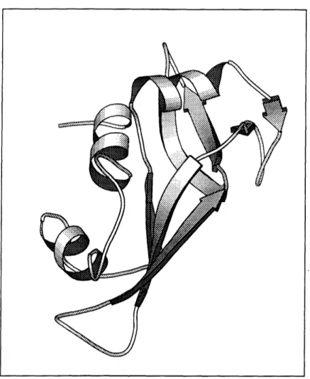
The first protein structure, myoglobin, was determined by means of X-ray crys-tallography [Kendrew and others, 1958]; see Figure 1-6, which was produced by the Molscript program [Kraulis, 1991]. People were dismayed at the apparent spatial disorder within each protein molecule. The protein shapes were a far cry from the regular repetitive packing that had been imagined.
On the other hand, there were a few encouraging aspects of protein structure. First of all, the predicted helix and strand structures did occur quite often in the proteins. Figure 1-7 shows a diagram of the backbone of ribonuclease A, containing both helices and sheets. The way the individual helices and strands packed together was not planar or regular, and much of the protein molecule looped around in very
Figure 1-6: The first observed protein structure. Myoglobin has 153 residues. Only the non-hydrogen backbone atoms are shown. Black spheres represent oxygen atoms; grey spheres represent carbons; white spheres represent nitrogens. Drawn by the Molscript program.
Figure 1-7: Structure of Ribonuclease A. The backbone of the protein is shown, with alpha (helices) and strand (arrows) regions shown. Drawn by the Molscript program. irregular shapes. The helices and strands themselves were often twisted, bent or kinked.
In spite of the seeming irregularity of the protein structures, a given sequence of amino acid residues always seemed to fold to the same complex structure. It was shown that ribonuclease and other proteins could be denatured and refolded to their native structure [Anfinsen et al., 1961]. This fact was tantalizing. It suggested that there must be some way to model the forces at work on and in the protein, such that one could predict the protein's three-dimensional structure from its amino acid sequence.
INPUT: sequence A C D I L E K L M Y ...
OUTPUT: secondary -h h h h - s s s s...
structure
Figure 1-8: The secondary-structure prediction problem. Secondary structure labels are h" (helix), "s" (strand), and "-" (other).
1.2.1 Secondary structure prediction
The fascination with helices and strands, the local structure found throughout pro-teins, has continued unabated. A hierarchy of protein structure description was de-fined. The first level, primary structure, is defined as the sequence of amino acid residues in the protein. Secondary structure is defined to be the local protein struc-ture. for example. strands and helices. Tertiary structure is the conformation of one protein: the three-dimensional positions of all the protein's atoms.
Much effort has been focussed on the prediction of secondary structure (Figure
1-8). In this problem, the goal is to find the type of secondary structure in which each
residue in the protein occurs. The input is the amino acid sequence of the protein. Early modelis of protein folding were based on the idea of secondary structure nu-cleation followed by propagation in a zipper-like effect along the protein chain [Zimm
and Bragg, 19,59. Lifson and Roig, 1961]. These models were used to interpret real folding data on polypeptides [Scheraga, 1978]. The Chou-Fasman model is a
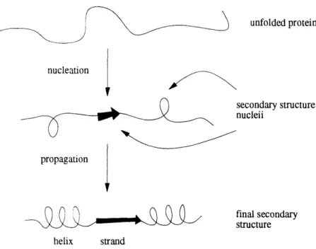
good example of a prediction algorithm based on the nucleation-propagation folding model [Chou and Fasman, 1978]. The basic idea was that short stretches of residues in the protein might strongly favor one of the secondary structures, and act as nu-cleation sites for those structures. The structures would then be extended along the chain until they ran into other amino acid residues which were strongly disfavorable to that type of structure. The extent to which an amino acid "favored" a particular type of secondary structure was determined by counting the number of occurrences of each amino acid in each type of secondary structure in a set of known-structure
unfolded protein nucleation secondary structure nucleii propagation i final secondary structure helix strand
Figure 1-9: The secondary structure nucleation-propagation model heavily influenced early protein structure prediction methods.
proteins.
Many different secondary-structure methods have been tried. Most of these ap-proaches are statistically based, relying on numbers culled from the database of known protein structures. Algorithms were developed based on information theory [Garnier
et al., 1978, Gibrat et al.. 1987], neural networksHolley89,Qian88,Stolorz91,Bohr88,
pattern-matching [Cohen et al., 1986], machine learning [King, 1988], and Markov
random fields [Collin Stultz and Smith, 1993]. Variations were tried in the definitions of secondary structure, in the input sequence representations, and in the types of additional information provided to the algorithm [Kneller et al., 1990, McGregor et
al., 1989, Levin et al., 1993. Niermann and Kirschner, 1990, Rost and Sander, 1993a].
People observed that there seemed to be an upper barrier to the accuracy with which secondary structure could be predicted from sequence information (about 65% residues correctly predicted for three secondary structure states: helix, strand, and other). There are several possible explanations for this limit. There might not be enough structure data yet to accurately determine the empirical parameters used in the predictions [Rooman and Wodak, 1988]. There might be sufficient informa-tion but the models themselves are faulty. Or it might be that secondary
struc-
hhh--in immunoglobulhhh--in
LTSGG
in serine protease
Figure 1-10: The same local sequence folds to different secondary structures in dif-ferent proteins, from Argos, 1987.
ture is not determined by secondary sequence alone. Clever computational exper-iments were performed to try to distinguish between these possibilities. Exam-ples were found of short amino acid sequences that had different secondary
struc-tures in different proteins (Figure 1-10) [Kabsch and Sander, 1984, Argos, 1987,
Sternberg and Islam, 1990]. Most of these results pointed toward the explanation that secondary sequence information is not sufficient to uniquely determine secondary structure. The conclusion was that tertiary structure interactions between amino acid residues very far apart in sequence but close in space must be crucial in determining secondary structure.
1.2.2 Tertiary structure prediction
Even if we discovered a way to determine secondary structure perfectly, or were told the answer by an oracle, we would not be done. We want to know the overall structure of the protein, not just the secondary structure.
One strategy is to start from the results of secondary structure prediction.
Peo-ple have worked on the problem of packing together strands and helices into a full
three-dimensional protein structure [Cohen et al., 1979, Cohen and Kuntz, 1987, Hayes-Roth and others, 1986]. This approach has the potential for dealing with the problem of ambiguous or inaccurate secondary-structure prediction, by following mul-tiple hypotheses, or by providing feedback to the secondary-structure predictor from the packing algorithm.
Another model of protein folding is strongly related to this approach of packing secondary structure pieces. The notion of building up a protein structure step by
unfolded secondary intermediate folded
protein structure conformation protein
formed
Figure 1-11: The pathway model of protein folding.
step was bolstered by the prevalent notion in the biochemical literature of folding intermediates. Levinthal [Levinthal, 1968] phrased the following argument: the con-formational space of a protein is too vast to be searched in a reasonable time by a protein. A possible conclusion is that there must be some specific folding pathway, with one or a few intermediate conformations that every folding protein visits (Fig-ure 1-11). Experimentalists found ways to trap and characterize protein species (or collections of conformations) that they described as intermediate conformations on the folding pathway [Creighton, 1978, Bycroft et al., 1990, Matouschek et al., 1990, Nail, 1986, Weissman and Kim, 1991]. The partially-packed protein structures in the secondary-structure-packing prediction methods are reminiscent of this idea of folding intermediates.
We probably understand enough about atoms and molecules to correctly model, with quantum mechanics, the structure of a protein. To determine the structure, you would solve the wave equation for the entire molecule and use a partition function to find low-energy solutions for atomic positions. Unfortunately, for proteins this calculation is not practical analytically, and prohibitively expensive computationally.
People have developed approximate energy functions for proteins that estimate the molecule's potential energy as a function of position [Karplus and Petsko, 1990]. It has been postulated that the folded protein is at a global or local minimum of these energy functions. The model incorporates interactions between atoms in the molecule, and biases bond lengths and angles toward a few favored positions. These
sequence Q R E T - - F N S I Q L E V - - N T ...
sequence 2 Q - D T P N H N S V - L D I M H R S ...
Figure 1-12: Two protein sequences are aligned to maximize the similarity between aligned amino acid residues.
energy functions are used to help determine protein structures from X-ray diffraction data. The energy function can be used to model the motion of a protein in time, but the model is too complex to allow simulation of motion for the time that it would
take the protein to fold.
People tried to simplify the energy function and protein structure representation in order to allow simulations which would model a long enough period of time to simulate the folding of a protein [Levitt and Warshel, 1975, Godzik et al., 1992, Hagler and Honig, 1978. Kuntz et al., 1976, Skolnick and Kolinski, 1990]. Instead of modeling all the atoms in the molecule, amino acid residues (which have ten or twenty atoms) are represented by one or two super-atoms. Forces between atoms are replaced by mean forces between amino acid residues. The motion of the molecules is restricted in various ways to simplify computation. For example, in some schemes only movements on a lattice are allowed.
One problem with these simplifications is that it is difficult to determine whether the model has been simplified to the point of losing important information. Simplified protein dynamics is not currently a viable means of predicting protein structure.
Another approach is to align the protein sequence to the similar sequence of a known-structure protein. if one exists (Figure 1-12). A model for the protein is then built based on the known structure of the other protein. This approach is known as homology modeling, and is currently the most successful protein structure prediction method [Lee and Subbiah, 1991].
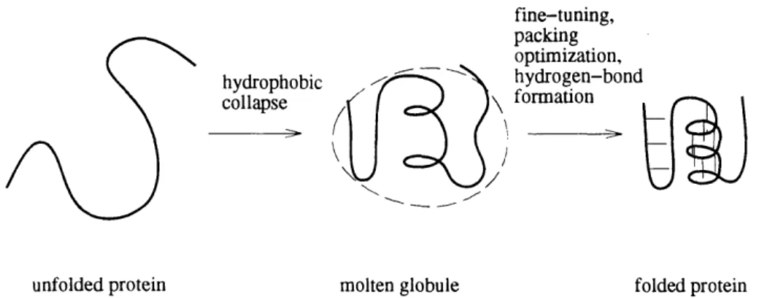
In the 1980s the 'hydrophobic collapse" theory of protein folding gained favor in the field. According to this theory, a protein folds in two phases. In the first phase, the unfolded protein chain collapses quickly to a fairly compact shape, called a molten globule, and this phase is driven by the tendency for hydrophobic ("water-fearing") amino acids to avoid water and clump together. The molten globule contains some
hydrophobic collapse _ fine-tuning,
hrogn-bn
optimization, hydrogen-bond formationI
unfolded protein molten globule folded protein
Figure 1-13: The hydrophobic collapse model of protein folding proceeds in two stages. secondary structure (strands and helices) and has roughly the fold of the final struc-ture, but is larger. In the second phase of folding, fine tuning occurs as the protein chain adjusts to optimize interactions between atoms. The result is a tightly packed structure, characteristic of observed folded proteins. There is now much experimental support for the hydrophobic collapse folding theory.
At this same time, people began looking for ways to judge the quality of a pro-posed protein structure. These methods were strongly influenced by the hydrophobic collapse folding model. A well-folded protein was modeled to have charged and po-lar (partially charged) parts of the protein on the outside, and hydrophobic parts on the inside (Figure 1-14). "Pseudopotential" functions were developed to incor-porate this idea. These functions are similar to the simplified energy functions used in protein folding simulations. Experiments were done showing that pseu-dopotential functions could discriminate between correct and incorrect structures for
one sequence [Baumann et al., 1989, Chiche et al., 1990, Holm and Sander, 1992,
Vila et al., 1991].
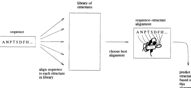
This discrimination by means of a pseudopotential function between correctly folded and misfolded proteins led naturally to an extension of homology modeling in which sequences were compared directly to a set of candidate structures [Wodak and Rooman, 1993, Blundell and Johnson, 1993, Fetrow and Bryant, 1993]. First the sequence is aligned onto each candidate structure, then the pseudopotential is used to determine which sequence-structure alignment is the correct one (Figure 1-15). This
hilic (water-loving) es on the outside
hydrophobic (water-hating) residues on the inside
Figure 1-14: Sketch of a correctly folded protein.
approach is currently very popular. It is sometimes referred to as inverse folding: instead of predicting structure from sequence, we have a pseudopotential function to evaluate how likely the sequence is to have been "generated" by a structure. The sequence-structure alignment is called threading because the sequence is threaded onto (aligned with) each structure. Arguments have been made, based on the fraction of new additions to the structure database which represent truly new folds, to the effect that we have seen a large fraction of all protein structures, and therefore the threading prediction method is likely to succeed in a large number of cases. The structure database might also be expanded by constructing hypothetical structures out of pieces of known structures.
Many threading pseudopotentials have been formulated. Pseudopotential func-tions were originally based on the hydrophobic collapse folding model. A numerical value was assigned to each amino acid type to represent its hydrophobicity; this num-ber was based on chemical experiments with a single amino acid type, or on statistical analyses of the known-structure database. In addition, each residue position in the structure has a numerical degree of exposure to the solvent. The pseudopotential functions compared the exposure of a residue's position to the residue's hydrophobic-ity, and assigned a low energy to buried hydrophobic residues and exposed hydrophilic residues.
Once the idea of a pseudopotential function for evaluating sequence-structure
library of structures sequence IANPTSDFH... align sequence sequence-structure alignment choose best alignment
to each structure predict
in library structure
based on this alignment
Figure 1-15: The threading method of tertiary structure prediction.
alignments was established, people experimented with incorporating other types of information in the pseudopotentials. These included:
* A residue's propensity to be in each type of secondary structure type (for exam-ple, does the residue "prefer" helix secondary structure over strand secondary structure?). This harks back to the early focus on secondary structure predic-tion.
* A residue's interaction with neighboring residues in the structure. Not only sequence-local neighbors, but neighbors distant in sequence but close in space could now be modeled. This was an exciting development, because it would seem to provide a way around the limitation imposed by considering only local sequence information in structure prediction.
Research on the inverse folding approach to structure prediction is actively being pursued at present. It is too early to determine the success of this method.
1.3 My work
The focus of my work is the question, "What makes for a good representation of
protein sequence and structure for structure prediction algorithms?" In carrying out
ANPTSDFH...
\\<\
j
this research, I am particularly interested in distinguishing the underlying models of protein folding that have influenced the structure prediction work. My approach is to compare different possible components of a protein representation. I consider a particular type of representation, in which each residue position in the database of known structures is labeled with a set of attributes. These attributes might include, for example, secondary structure type, solvent exposure, or amino acid. I use a statistical technique called contingency table analysis that allows one to tease out the relative importance of, and interaction between, the different types of information in a representation of events. In my work, the events of interest are the residue positions in the structure database. I discuss implications of this analysis for protein structure prediction. I also consider the power of the protein representations in the contexts in which they will be used, by comparing their performances in secondary and tertiary structure prediction algorithms.
In the next sections, I highlight a few of the questions I investigated.
1.3.1 Hydrophobic collapse vs. structure nucleation and
propagation
My results show that a structure prediction algorithm based on the hydrophobic col-lapse model of protein folding should perform better than one based on secondary structure nucleation and propagation. In particular. I observe that amino acid type is more strongly correlated with solvent exposure than with secondary structure. This finding agrees with the currently popular hydrophobic collapse model of protein fold-ing: that the first and strongest effect is the burial of hydrophobic residues in the core of the structure. Thus, my results indicate that protein structure prediction representations should include an effective model of hydrophobicity and solvent ex-posure. For example, it might be useful to predict solvent exposure along the protein chain instead of the commonly used secondary structure as the first step in a two-step tertiary structure prediction method.
secondary structure propensities, it is a good idea to do so; secondary structure propensities do add useful information.
1.3.2 Modeling hydrophobic collapse
The hydrophobic effect has been modeled in various ways. What is really going on physically is complicated. Polar solvent molecules around exposed hydrophobic residues in the protein lose hydrogen-bonding partners. On the other hand, buried polar residues may miss chances to make good hydrogen bonds. One model of the hydrophobic effect creates a fictitious hydrophobic force, in which hydrophobic atoms or residues attract one another. This pairwise interaction model is used by Casari and Sippl, for example [Casari and Sippl, 1992]. An alternative approach (for example,
Bowie and colleagues [Bowie et al., 1991]) looks at each residue in isolation as a
singleton term in the pseudopotential and asks how hydrophobic it is and how much water it sees. If the residue is buried and hydrophobic, or exposed and hydrophilic, then the residue is happy. Which approach is better, pairwise attractive force or singleton solvent exposure?
I compare the pairwise model to the singleton model of hydrophobic collapse. The former examines the correlation between the hydrophobicities of neighboring amino acids; the latter examines the correlation between an amino acid's hydrophobicity and its solvent exposure. My analysis shows that looking at the association between amino acid type and solvent exposure at a single site is more informative than looking at the association between pairs of amino acids. The implication is that it is a good idea to model the hydrophobic effect as a first-order correspondence between amino acid hydrophobicity and solvent exposure, as opposed to as the second-order effect which is the pairing of similar types of amino acids. This turns out to be a very useful result for threading algorithms, because threading with first-order effects can be done quickly, while threading with pairwise effects is computationally expensive [Lathrop,
1.3.3 Pairwise interactions: great expectations
Many designers of pseudopotential functions assume that modeling of pairwise, triplet, and even higher-order interactions between residue positions in protein structures is necessary to distinguish misfolded proteins from correctly folded proteins. Threading methods incorporating high-order residue interactions have been developed based on this assumption.
Statistical arguments have been made about the relative importance of the higher-order terms to the singleton terms, and it was shown that in theory the pairwise terms should provide half again as much information as the singleton terms [Bryant and Lawrence. 1993]. What happened in practice? While little has been published comparing the performance of singleton to higher-order pseudopotentials, preliminary results indicate that pairwise terms do not improve the threading results. Why would this be? Perhaps the models are inadequate, or the pseudopotentials are incorrect in
somIe waV.
The analysis that I performed shed some light on the question of the importance of pairwise interactions in threading.
First of all, my statistical analysis at first glance suggests that pairwise terms should improve the threading results. They contain information not available in the single-residue attributes. In fact, by one way of measuring, the pairwise terms should contain half again as much information as the singleton terms.
However. a closer examination of the statistics shows the pairwise terms in the pseudopotential scoring functions are plagued by severe problems with low sample size. The pairwise terms do contain some additional useful information, but with low sample sizes it is swamped by noise.
To compensate for the noise, there are several things that can be done. One approach is to reduce the complexity of the data representation. I grouped the 20 amino acids into three groups based on their hydrophobicity. When I do this I have adequate sample sizes, but the singleton terms are now far more important than the pairwise terms. This could be due to the fact that the representation is too coarse, or it might be a more accurate representation of the true relative importance of pairwise
and singleton terms, or some combination of the two.
I also find that some information is accounted for by the preference of an amino acid for its neighbor's solvent exposure. This effect is not modeled by current pseu-dopotential functions that model pairwise interactions.
1.3.4 Amphipathicity
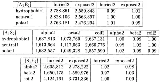
In looking at pairwise occurrences of amino acids, I discovered an unexpected cor-relation between hydrophobicity types on opposite, non-contacting sides of buried beta sheets. This might represent a sequence signal for beta strand conformation. Regardless of the reason, this, along with the other results about the importance of solvent exposure, suggested to me that I might try to incorporate some sort of amphipathicity constraint in structure prediction algorithms. I found that providing amphipathicity information to a neural net that predicts secondary structure improves its performance by a small but significant amount.
1.4 Outline of thesis
Chapter 2 describes the protein representations I use in the thesis, and gives some background on the analysis of contingency tables using loglinear models. The next four chapters (3-6) apply contingency table analysis to single-residue properties, paired residues, single residue in parallel and antiparallel beta sheets, and pairs of residues in beta sheets. The next two chapters evaluate protein representations by using them in programs that operate on proteins. In Chapter 7, I use various sequence representations as input to a neural network that predicts secondary structure. In Chapter 8, I use various structure representations in the threading program to align a structure to a sequence. In Chapters 9 and 10, I describe work in progress and sum-marize my conclusions. Appendix A describes some related work in protein statistics and threading.
Chapter 2
Background
In this chapter, discuss the protein representations employed in this thesis. Then I introduce contingency table analysis, the statistical method that I use extensively in Chapters 3 through 6, and which is closely related to the pseudopotential functions I
test; in Chapter 8.
2.1 Knowledge representation
In this section, I discuss the particular types of knowledge representation that I consider for protein sequences and structures. I consider a residue to be the basic unit of protein structure. I represent a protein as a string of residues. Each residue has a set of attributes. In addition, the protein representation may include a list of pairs of residues that are related in some way, and each residue pair may have attributes above and beyond the individual residues' attributes. I refer to the attributes of a single residue as "singleton" attributes; those of a residue pair are "pairwise" attributes.
Each attribute can take on one of a finite set of values. A given residue is catego-rized by one and only one value for each of its attributes. Thus the attribute values are complete and non-overlapping. On occasion I compare or use attributes that are generalizations or specializations of each other. An attribute Al is a generalization
of an attribute A2 if for any two residues ri and rj,
(A2(ri) = A2(rj)) =' (Al(ri) = Ai(rj)),
where Aj(ri) is the value of attribute Al for residue ri (and so on). In other words, if A2 classifies two residues as having the same attribute values, then Al must also.
2.1.1 Single residue attributes
The attributes of a residue that I investigate include solvent exposure, secondary structure, and sequence.
Solvent exposure
Solvent exposure specifies the amount of a residue's surface area that is exposed to the solvent on the outside of the protein. In this thesis, the possible solvent exposure values are {buried, exposed).
The solvent exposure is computed by the DSSP program using geodesic sphere integration [Kabsch and Sander, 1983]. Points on the surface of a sphere of radius equal to the sum of the radii of an atom and a water molecule are considered exposed if the water sphere centered there does not intersect with any other protein atom. The total area of these points for a residue are computed by summing over a polyhedron made of approximately equal triangles. The atomic radii are taken to be 1.40 for
0. 1.65 for N, 1.87 for Ct, 1.76 for the carbonyl C, 1.8 for all side-chain atoms, and
1.4 for a water molecule. The number reported by the DSSP program is the average number of molecules in contact with each residue, which is estimated from the surface area by dividing by 10 square Angstroms.
I compute relative solvent exposure by dividing the DSSP solvent exposure by the maximum exposure for each residue, as recorded in Section B.3.
I apply a threshold of 20% to the relative solvent exposure to determine the buried and exposed labels.
Secondary structure
I use the DSSP definitions of secondary structure types alpha helix and beta
strand [Kabsch and Sander, 1983]. All other residues are labeled coil. In some
of the analysis, I further divide the beta strand category into parallel and
antipar-allel; this is a specialization of the {alpha, beta, coil} attribute.
The DSSP program finds alpha helix and beta strand by first determining the locations of backbone hydrogen bonds. Hydrogen bonds are determined by placing partial charges on the C (+.42e), O (-.42e), N (-.2e), and H (+.2e) atoms. The electrostatic interaction energy is calculated as
1 1 N
E = f(.42e)(.2e)[ -
-
]
rON rCH roH rCN
where f is a dimensional factor to translate from electron units to kcals, f = 332, and E is in kcal/mol. e is the unit electron charge. The distance between atoms of type i and j, r, is in angstroms. A hydrogen bond is said to exist if E is less than the cutoff -0.5 kcal/mol.
DSSP defines a "bridge" as existing between two nonoverlapping stretches of three residues each if there are two hydrogen bonds characteristic of beta structure
(Fig-ure 2-1). A "ladder" is a set of one or more consecutive bridges of identical type, and a "sheet" is a set of one or more ladders connected by shared residues. A parallel
bridge aligns bridge residues in pairs as (i - 1,j - 1), (i,j), and (i + l,j + 1). An
antiparallel bridge aligns pairs (i - 1,j + 1), (i,j), and (i +
1,j
- I).Sequence
I use several representations for sequence. The simplest is the amino acid, which has 20 different values, one for each type of amino acid found in proteins. I also (following Lifson and Sander [Lifson and Sander, 1980]) group the amino acids by hydrophobic-ity, obtaining three classes hydrophobic, neutral, and polar. Lifson and Sander use two other groupings that I employ in Chapter 6 on pairwise interactions in beta sheets. These grouped representations are generalizations of the 20-valued amino acid
N H O=C C C C=O -- H N H N C=O C C O=C C HN I NH C C=O C-O -H N C C O=C N H --C C=O NH O=C C
HN
(a) N O=C C HN (b)H ---
O=C
NH C C=O (c)Figure 2-1: Bridges between beta strands. (a) and (c) are antiparallel bridges; (b) is a parallel bridge. A bridge exists between two nonoverlapping stretches of three residues each of there are two hydrogen bonds characteristic of beta structure. Hydrogen bonds are shown dashed; covalent bonds are shown as solid lines; the sidechains are not represented in this diagram.
type attribute.
In the threading chapter (Chapter 8), I consider a representation in which each
residue has an attribute representing its local sequence. This is a specialization of the 20-valued amino acid type attribute. For a local sequence window of 13, for example, there are 2013 possible values of this attribute.
2.1.2 Attributes of residue pairs
I consider a number of different residue pair attributes.
Sidechain contact
I calculate whether or not the sidechains of the residues are in contact. There are two values for this attribute: in-contact and not-in-contact.
Topological relationship
For pairs that occur in beta sheets, I consider the following types:
1. Beta pairs. My definition of a beta pair is the two central residues in a bridge
(for a definition of bridge, see Section 2.1.1). I sometimes further specialize the beta pairs into parallel and antiparallel beta pairs.
2. Diagonal pairs. If (i,j) and (i + 2,j + 2) are both 3p pairs, then (i,j + 2) and
(i + 2, j) are diagonal pairs (denoted by 6p). If (i, j) and (i + 2, j - 2) are A,
then (i,j - 2) and (i + 2,j) are EA. I sometimes further specialize these into
parallel and antiparallel diagonal pairs.
:3. (i, i + 2) pairs. Residues i and i + 2 are in a beta strand.
2.2 Contingency table analysis
This section provides an overview of contingency table analysis. There are a number of books on the subject; I have found the Wickens text to be particularly useful [Wickens,
2.2.1
Contingency tables
Contingency table analysis is used to analyze counts of objects or occurrences, where each object has several attributes. It is well-suited for analyzing counts of residue occurrences in a set of known-structure proteins.
My data describes residues or residue pairs in protein structures. Each residue or pair has several attributes that describe its sequence and structure characteristics. Each of these attributes (such as secondary structure) has several possible values (such as alpha, beta, or coil), and each object has one and only one value for each attribute. In the statistics literature, data composed of objects with such attributes is called categorical data. If data objects have several attributes, the data is called
cross-classified categorical data. Tables of counts of cross-classified categorical data
are called contingency tables.
For example, to examine the relation between amino acid type, solvent exposure, and secondary structure type, I tabulate, for each residue in a protein, the residue's amino acid type, its exposure to solvent, and the type of secondary structure in which it appears. Thus I generate a three-dimensional contingency table. Each dimension of the table corresponds to one of the attributes.
2.2.2 Questions asked in contingency table analysis
Contingency table analysis can be used to answer questions about conditional in-dependence and the strength of statistical relationships between variables. In this thesis, the following questions exemplify the issues that can be addressed using this statistical technique:
* Is amino acid type related to solvent exposure? In other words, are there statistically significant preferences of some amino acid types for being buried or exposed?
* Are solvent exposure and secondary structure jointly more predictive of amino acid type than either alone?
* Which is stronger: the correlation between amino acid type and solvent expo-sure, or the correlation between amino acid type and secondary structure? * Are there some pairs of amino acids that show a preference to occur in
neigh-boring positions in the protein structure? If so, is this preference dependent on the structural attributes of the residue positions in the protein?
2.2.3 Models of data
In contingency table analysis, a model of the data is used to create a table of expected counts. This expected count table is compared to the table of observed counts, and a standard statistical test is used to determine whether there is a significant difference between the expected and actual counts. The null hypothesis asserts that the model explains the data; the statistical test can determine if this hypothesis is false. It cannot prove that the model does fit the data, because it might be that there is not enough data to make the determination.
A model can be compared not only to the observed data, but also to another model. This is useful in determining relationships between various elements of the model.
There are many possible models for the data in a contingency table. I use a type of model called hierarchical loglinear models. These models are nice because they can be used to frame the types of questions that I would like to ask about the data.
Hierarchical loglinear models are explained in more detail below, in Section 2.2.5. There are many possible hierarchical loglinear models for a given contingency table. It is important, therefore, to have specific questions in mind when performing the analysis.
The meaning of the models and the relationships between the models must be supplied by the person doing the analysis. The results of contingency table analysis are often interpreted to support an assertion about causality. The statistical analysis does not intrinsically say anything about which attribute "causes" which other, but rather makes a simpler statement about the co-occurrence of events. Any meaning
Color
red
green
total
Price
low high total
NLR NHR NR NLG NHG NG
NL NH N
Table 2.1: Form of a two-dimensional contingency table. must be imposed by the person interpreting the results.
2.2.4 A simple contingency table example
Suppose we want to analyze the attributes of different apples. We have a large barrel of apples on which we will base our analysis. Each apple in the barrel has the following attributes: color and price. Each attribute has a set of possible values, as follows.
* Color: red, green. * Price: high, low.
To build a contingency table, we tip over the barrel and record the number of apples for each possible combination of attributes. In this case there are four (low-priced green, high-(low-priced green, low-(low-priced red, and high-(low-priced red). We end up with
Table 2.1, which has one cell for each attribute combination.
The total number of apples with the various color and price attributes are written in the margins of the table. The cell which is the margin of the margins contains the total number of counts, N. Our model of independence generates a table of counts in which the margin totals are the same as in the observed table, but the entries in the table are computed from the marginal counts, or totals. This is because the margin counts are what we use to determine the independent probabilities of color and price.
Testing for independence
How can we test the hypothesis that an apple's color is independent of an apple's price? We estimate the probability that an apple is red from the observed frequency


![Table 4.4: Non-contacting pair marginal counts: partner's same attribute. [S 1 S 2 ] shows a strong dependency between secondary structure types of non-contacting residues](https://thumb-eu.123doks.com/thumbv2/123doknet/14174026.475009/78.940.257.725.126.407/contacting-marginal-attribute-dependency-secondary-structure-contacting-residues.webp)