Calibration of Dynamic Traffic Assignment Models with
Point-to-Point Traffic Surveillance
by
Vikrant Vaze
Bachelor of Technology in Civil Engineering
Indian Institute of Technology, Bombay, India (2005)
Submitted to the Department of Civil and Environmental Engineering
In partial fulfillment of the requirements for the degree of
Master of Science in Transportation
at the
MASSACHUSETTS INSTITUTE OF TECHNOLOGY
June 2007
© Massachusetts Institute of Technology 2007. All rights reserved.
Author...
...
Department of Civil and Environmental Engineering
May 30, 2007
C ertified b y ...
....
Moshe E. Ben-Akiva
Edmund K. Turner Professor of Civil and Envir.nmental Engineering
ThesisSuperyisor
Accepted by...
MASSACHUSETTS INSTITUTE OF TECHNOLOGYJUN 0 7 2007
Daniele Veneziano
Chairman, Departmental Committee for Graduate Students
Calibration of Dynamic Traffic Assignment Models with
Point-to-Point Traffic Surveillance
by
Vikrant Vaze
Submitted to the Department of Civil and Environmental Engineering on May 30, 2007, in partial fulfillment of the
requirements for the degree of Master of Science in Transportation
Abstract
Accurate calibration of demand and supply simulators within a Dynamic Traffic Assignment (DTA) system is critical for the provision of consistent travel information and efficient traffic management. Emerging traffic surveillance devices such as Automatic Vehicle Identification (AVI) technology provide a rich source of disaggregate traffic data. This thesis presents a methodology for calibration of demand and supply model parameters using travel time measurements obtained from these emerging traffic sensing technologies.
The calibration problem has been formulated in two different frameworks, viz. in a state-space framework and in a stochastic optimization framework. Three different algorithms are used for solving the calibration problem, a gradient approximation based path search method (SPSA), a random search meta-heuristic (GA) and a Monte-Carlo simulation based technique (Particle Filter). The methodology is first tested using a small synthetic study network to illustrate its effectiveness. Later the methodology is applied to a real traffic network in the Lower Westchester County region in New York to demonstrate its scalability. The estimation results are tested using a calibrated Microscopic Traffic Simulator (MITSIMLab). The results are compared to the base case of calibration using only the conventional point sensor data. The results indicate that the utilization of AVI data significantly improves the calibration accuracy.
Thesis Supervisor: Moshe E. Ben-Akiva
Acknowledgements
I am highly grateful to a lot of people for making my stay at MIT such a memorable
experience. I would like to thank my advisor Prof. Moshe Ben-Akiva for his guidance and inspirational presence throughout the course of my work at MIT. I would also like to express my gratitude towards Constantinos Antoniou and Yang Wen for providing incessant help related to all my transportation and IT questions. I am especially thankful to Constantinos for spending so much effort and time to ensure that I understand the concepts. I am highly indebted to Prof. Nigel Wilson for his guidance and friendly advice from time to time regarding many academic issues.
I express my deep sense of gratitude to all the ITS lab members, for being so helpful and
friendly and making the stay in the lab a thoroughly enjoyable experience. I would like to especially thank Vaibhav and Varun for always being there in every good and bad experience over the last two years. Senior students in the lab including Rama, Charisma, Maya and Yang have been great sources of knowledge and helped me at every step on issues related to research, coursework and thesis writing. Charisma with her PhD comics perspective on virtually every topic, Maya with her socialization fundaes and Yang with his 'Jianzi' coaching have been amazing. Ramachandran Balakrishna, Charisma Choudhury, Yang Wen, Anita Rao, Gunwoo Lee, Vaibhav Rathi, Varun Ramanujam, Maya Abou Zeid, Shunan Xu, Casper Chorus, Emma Frejinger and of course, Leanne Russell, have all made the ITS lab a vibrant, lively place.
I would like to thank Tanachai Limpaitoon and Onur Aydin for their friendship and
support during difficult days. I am thankful to my MST classmates including Carlos, Celia, Grace, Hong Yi, Joanne, Nobuhiro, Ritesh, Tanachai and Valerina for making this journey truly world class. It's impossible to forget the junta2005. I would like to thank Chetan, Saumil, Parikshit, Deep, Deepanjan, Shrikanth, Ashish, Ram, Srujan, Nidhi, Harish, Sudhir and Sukant who have made the MIT life a fantastic experience.
Most importantly I would like to thank my parents and sister, without whose unwavering support, nothing could have been possible. Finally I thank god for giving me this opportunity.
Contents
1. Introduction...
13
1.1 Dynam ic traffic assignm ent system s ... 14
1.2 N eed for DTA calibration ... 15
1.3 Thesis m otivation and problem statem ent ... 16
1.4 Im plem entation fram ework... 17
1.5 Thesis contribution... 18
1 .6 T h esis o u tlin e ... 2 0
2. Literature R eview ...
21
2.1 U se of AV I data in previous studies ... 21
2.2 Stochastic optim ization based studies... 27
2.3 State-space formulation based studies ... 29
2 .4 S u m m ary ... 3 3
3. Automatic Vehicle Identification Technology ...
35
3.1 Introduction... 35
3.2 AVI inform ation types ... 37
3.3 Sum m ary ... 41
4. Problem Form ulation ...
43
4.1 Optim ization form ulation... 43
4.1.1 N otation... 43
4.1.2 Form ulation... 44
4.2 State-space formulation ... 45
4.2.1 State estim ation for dynam ic system s... 46
4.2.2 State-space formulation for the traffic network ... 47
4.3 Sum m ary ... 49
5.
Solution A lgorithm s...
51
5.1 Stochastic optimization approaches for simulation based systems... 51
5.2 Classification of optim ization algorithm s... 52
5.3 Path search m ethods... 53
5.3.1 Response surface m ethodology... 53
5.3.2 Stochastic approxim ation... 55
5.4 Pattern search m ethods ... 59
5.4.1 Hooke and Jeeves m ethod... 59
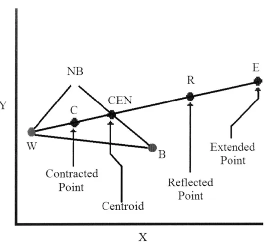
5.4.2 Downhill sim plex m ethod... 60
5.5 Random search m ethods ... 64
5.5.1 Sim ulated annealing... 64
5.5.2 Genetic algorithm s ... 66
5.6 Solution algorithm s for state-space formulation... 71
5.8 Extensions of K alm an filtering technique... 73
5.8.1 Extended Kalm an filter ... 74
5.8.2 Iterated extended Kalm an filter ... 75
5.8.3 Lim iting extended K alm an filter... 75
5.8.4 Unscented K alm an filter ... 76
5.8.5 Particle filter... 77
5.9 Choice of candidate algorithm s ... 81
5 .10 S u m m a ry ... 8 2
6. Comparative Assessment of Algorithms on Synthetic Network... 83
6.1 Objectives ... 83
6.2 Sim ulation of AV I sensors... 84
6.2.1 DynaM IT m odifications... 84
6.2.2 Post processing... 85
6.3 Experim ental design... 85
6.3.1 Study netw ork ... 86
6.3.2 Calibration param eters ... 86
6.3.3 Sensors ... 87
6.3.4 Starting param eter values... 88
6.3.5 M easures of goodness-of-fit ... 89
6.4 Im plem entation details... 91
6.4.1 SPSA im plem entation... 91
6.4.2 GA im plem entation... 93
6.4.3 Particle filter im plem entation ... 95
6.5 Habitual link travel tim es ... 97
6.6 Calibration results ... 99
6.6.1 Dem and-only calibration ... 99
6.6.2 Sim ultaneous dem and-supply calibration ... 104
6.7 Sensitivity analysis... 111
6.8 V alidation... 113
6.9 Sum m ary ... 114
7.
C ase Study: Low er W estchester C ounty ...
1 17
7.1 Objectives ... 1177.2 Experim ental design... 118
7.2.1 Study netw ork ... 118
7.2.2 V ehicle m ix... 121
7.2.3 Calibration param eters ... 122
7.2.4 Sensors ... 123
7.2.5 Starting param eter values... 124
7.3 Im plem entation details... 124
7.4 Habitual link travel tim es ... 125
7.5 Calibration results ... 125
7 .7 S u m m a ry ... 1 3 7
8 . C o n c lu sio n ...
13 9
8.1 Major findings and research contribution... 139
8.2 Directions for future research ... 142
Appendix A : Overview of DynaM IT ...
143
A .1 In tro d u ctio n ... 14 3 A.2 Features and functionality... 144
A .3 O verall fram ew ork ... 14 5 A.4 Prediction and guidance generation ... 151
Appendix B: Overview of M ITSIM Lab ...
155
Appendix C: MATLAB Code for SPSA Algorithm ...
157
Appendix D : M ATLAB Code for Genetic Algorithm ... 161
Appendix E: MATLAB Code for Particle Filter Method ... 167
List of Figures
Fig 3.1: Effectiveness of AVI information ... 40
Fig 5.1: An iteration of the downhill simplex method... 61
Fig 5.2: Single point crossover ... 68
Fig 5.3: T w o point crossover ... 68
Fig 5.4: C ut and splice crossover... 69
Fig 6.1: Sm all netw ork topology ... 86
Fig 6.2: Roulette wheel selection operator ... 94
Fig 6.3: Single point crossover operator ... 95
Fig 6.4 : M utation operator ... 95
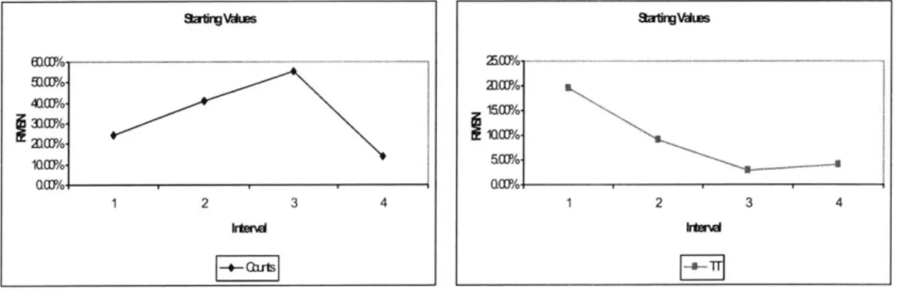
Fig 6.5: RMSN of starting parameter values ... 101
Fig 6.6: Calibration results: Demand-only calibration ... 102
Fig 6.7: Comparison of algorithms: Demand-only calibration without AVI data... 103
Fig 6.8: Comparison of algorithms: Demand-only calibration with AVI data... 103
Fig 6.9: Calibration results: Simultaneous demand-supply calibration... 106
Fig 6.10: Comparison of algorithms: Demand-supply calibration without AVI data .... 107
Fig 6.11: Comparison of algorithms: Demand-supply calibration with AVI data ... 107
Fig 6.12: Starting values of sensor counts ... 108
Fig 6.13: Sensor counts after demand-only calibration ... 108
Fig 6.14: Sensor counts after demand-supply calibration... 109
Fig 6.15: Starting values of travel tim es ... 109
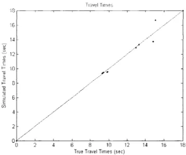
Fig 6.16: Travel times after demand-only calibration ... 110
Fig 6.17: Travel times after demand-supply calibration... 110
F ig 6 .18: S en sitivity an alysis ... 113
Fig 7.1: N etw ork description ... ... 119
F ig 7 .2 : S en sor lo cation s... 120
Fig 7.3: Proportion of commercial vehicles during the morning period... 122
Fig 7.4: Calibration results: Demand-only calibration of LWC network ... 128
Fig 7.5: Demand-only calibration without AVI data ... 129
Fig 7.6: Demand-only calibration with AVI data ... 129
Fig 7.7: Calibration results: Simultaneous demand-supply calibration of LWC network ... 1 3 1 Fig 7.8: Final demand-supply calibration without AVI data ... 132
Fig 7.9: Final demand-supply calibration with AVI data ... 132
Fig 7.10: Starting value of sensor counts... 133
Fig 7.11: Sensor counts after demand-only calibration ... 133
Fig 7.12: Sensor counts after demand-supply calibration... 134
Fig 7.13: Starting values of travel tim es ... 134
Fig 7.14: Travel times after demand-only calibration ... 135
Fig 7.15: Travel times after demand-supply calibration... 135
Fig A .1: T he rolling horizon ... 145
Fig A.2: The DynaMIT framework ... 147
List of Tables
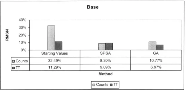
Table 6.1: Accuracy of demand-only calibration ... 101
Table 6.2: Accuracy of simultaneous demand-supply calibration... 105
T ab le 6 .3 : S en sitivity analy sis ... 112
Table 6.4: Validation results for synthetic network... 114
Table 7.1: Accuracy of calibration for LWC network ... 127
1. Introduction
In the recent years, transportation problems have been attracting a lot of attention. It is becoming increasingly important to ensure that the available means of transportation continue to function efficiently with minimal impact on the environment. Road transportation is one of the most critical means of transportation today, due to its pervasiveness as well as direct impacts on its surroundings. While the traffic load on highway transportation system is increasing at a tremendous rate, the growth in highway infrastructure is far slower. Construction of new highway capacity has not kept pace with increases in population and car use and the resulting increase in demand for highway travel. In the United States, between 1980 and 1999, the total length of highways increased by 1.5 percent, while the total vehicle-miles traveled during the same period increased by 76 percent (FHWA, 2006). Building new road infrastructure is becoming increasingly difficult while the congestion costs are growing rapidly. Therefore, in the recent years, the focus has shifted from building new infrastructure to efficient utilization of existing infrastructure. Innovative means are sought to solve the growing congestion problem. Intelligent transportation system is one of the technology-oriented solutions to traffic congestion.
Intelligent Transportation System (ITS) technologies aim to make use of recent advances in the field of communication, sensing and computation to better manage the available roadway infrastructure. Traffic sensing devices such ds loop detectors, video cameras, infrared sensors, Global Positioning System (GPS), radio frequency identification (RFID) tag readers etc have made the task of traffic measurement much more tractable. Traffic information devices such as Variable Message Signs (VMS), Highway Advisory Radio (HAR), in-vehicle navigation systems are now being used much more widely than before. Advances in semiconductor technology have made it possible to perform complex computations for traffic decision support at a great speed. Optimally managed highway traffic system, far from being a distant dream, is a foreseeable possibility today. Due to these technological advances, the development of highly accurate traffic prediction models and decision support systems is no longer just an academic exercise, but has the
potential to produce significant traffic improvements. Dynamic Traffic Assignment
(DTA) systems are viewed as the solution to the problem of accurate traffic estimation
and prediction.
1.1 Dynamic traffic assignment systems
Dynamic Traffic Assignment (DTA) systems are mathematical tools that are designed to provide decision support for traffic management and information provision. DTA systems aim to improve traffic conditions and alleviate congestion through accurate proactive forecasts of likely problems and future bottlenecks in the network. The traffic estimation and forecasts can be used by the traffic managers in two major ways. ATMS and ATIS are the tools available to traffic managers to manage traffic close to optimality.
Advanced Traffic Management Systems (ATMS) involve traffic control devices such as ramp meters, signal timings, variable speed limit signs and lane use signs to manage the flow of traffic through the supply side measures. On the other hand, Advanced Traveler Information Systems (ATIS) such as variable message signs, in-vehicle guidance units, traffic advisory through radio, television and internet can provide useful traffic information to roadway users and guide them to make more informed travel decisions for themselves, regarding destination, departure time, travel mode and route. Thus the ATIS manages the demand side of roadway networks. The DTA systems form the basis of these tools for traffic management through the management of demand and supply.
State-of-the-art DTA models have been developed in the past decade, for a variety of traffic network design, planning and operations management situations. These models employ sophisticated algorithms and detailed microscopic, macroscopic and mesoscopic simulation techniques to estimate current network performance, predict future conditions and generate traffic guidance.
packages include CORSIM (FHWA, 2005), PARAMICS (Smith et al., 1995), AIMSUN2 (Barcelo and Casas, 2002), MITSIMLab (Yang and Koutsopoulos, 1996; Yang et al., 2000), VISSIM (PTV, 2006) and Trans-Modeler (Caliper, 2006). These models, while being highly accurate, suffer from computation-intensiveness and that obviates the possibility of employing them for real-time traffic management purposes. At the other end of the spectrum are the macroscopic models such as METANET (Messmer and Papageorgiou, 2001), EMME/2 (INRO, 2006), VISUM (PTV, 2006) and the cell transmission model (CTM, Daganzo (1994)). They model traffic flow through road segments as fluid flow through pipes. The aggregate nature of traffic modeling makes them inappropriate for accurate modeling of traveler behavior in congested situations. Mesoscopic models try to strike a balance between the computational constraints for making them useful in real-time applications, and accuracy requirements to be able to describe the network conditions with adequate level of details. Examples of such systems include Dynamic Network Assignment for the Management of Information to Travelers (DynaMIT, Ben-Akiva et al. (2001, 2002)) and DYnamic Network Assignment-Simulation Model for Advanced Road Telematics (DYNASMART, Mahmassani (2002);
UMD (2005)).
1.2 Need for DTA calibration
In order to make effective traffic management decisions, the traffic managers need to know not only the current state of the system but also the predicted future states on a continuous basis. The better the knowledge about current and future state, the higher is the likelihood of effective decisions. However, in spite of the vast improvements in traffic sensing, it is impossible to measure each and every variable related to the state of the system at any point of time. While the sensors and historical knowledge about the network conditions do provide useful information, a substantial effort is necessary to estimate and predict various useful traffic performance indices which cannot be measured directly.
The DTA models provide a useful way to model the highway transportation system. However, the effectiveness of DTA models depends on the ability to replicate the network conditions accurately based on the available data. Various inputs and model parameters within the DTA system need to be set to appropriate values. Calibration is the process of assigning values to model parameters so as to replicate the traffic measurements closely.
1.3 Thesis motivation and problem statement
There is an abundance of literature related to calibration of DTA models, both the calibration of supply parameters as well as estimation of origin-destination flows. However, most of the studies in this area treat each model's parameters separately and focus on utilization of particular type of sensor data, most commonly link-flow counts. The reader is referred to Balakrishna (2006) for a detailed overview of literature related to the previous studies on calibration of specific demand or supply parameters using specific types of sensor data.
Several new types of traffic data collection technologies are being deployed in recent years, with a focus on disaggregate data collection. Different types of calibration approaches are necessary to suitably incorporate such wide variety of information. Hence, it is of value to focus on generic approaches that focus on calibration of various types of model parameters using a variety of traffic measurement technologies. A large set of these emerging technologies can be categorized as Automatic Vehicle Identification (AVI) technologies, which form the basis of this study. Note that the terms point-to-point sensor data and AVI data are sometimes used interchangeably. The two are not exactly the same and the readers are referred to section 3.1 for a discussion of the distinction between them. For the sake of simplicity, the term AVI data has been frequently used in this thesis.
to accommodate the calibration of any type of DTA model parameters using a variety of conventional and emerging traffic sensor measurement data. The calibration problem can be formulated as an optimization problem with the objective function representing a goodness-of-fit measure between observed (or apriori) values and the simulated values. The important constraints include those which express the fitted sensor measurements as a function of the calibration parameters and network characteristics. There may be other constraints providing lower and upper bound on the allowable values of the demand and supply parameters. Alternatively, the calibration problem can be formulated in a state-space framework which is described as the problem of estimating the state-vector using the measurement and transition equations. The calibration parameters constitute the state-vector describing the network conditions at any time interval. The sensor measurements provide the information necessary to estimate the state vector. The sensor measurements are functions of the state-vector values and the two are related by the indirect measurement equations. The apriori values are related to the state-vector by direct measurement equation. Further, the state-vectors across time periods are related to each other through the transition equations.
This thesis focuses on the calibration of DTA models using AVI data, under each of these two generic frameworks. A mesoscopic DTA system called DynaMIT is used to demonstrate the usefulness of the proposed methodology.
1.4 Implementation framework
As mentioned earlier, this thesis focuses on offline calibration of models and algorithm parameters within DynaMIT. A comparative analysis of three different algorithms is performed on a hypothetical network. The traffic sensor data is generated synthetically using a microscopic traffic simulator called MITSIMLab. However, in order to justify the usefulness of the approach, its effectiveness needs to be illustrated for calibration of a real traffic network with complex demand-supply interactions and large set of parameters. Therefore, a network from the Lower Westchester County (LWC) in New York State is chosen for demonstration. The LWC network has a set of loop detectors and toll booths
that together provide classified link flow counts. However, flow of AVI sensor data from the New York State Department of Transportation has yet not been established due to technical difficulties. Therefore, MITSIMLab is used as a proxy for this case study which can generate any necessary surveillance data that can then be made available for calibration of DynaMIT.
MITSIMLab is a microscopic traffic simulator that models traffic flow at the level of every individual driver. It uses behavioral algorithms and discrete choice models (Ben-Akiva and Lerman, 1985) to model decisions taken by an individual while traveling from his/her origin to his/her destination. Upon proper calibration with a network, MITSIMLab can effectively replicate the traffic characteristics. MITSIMLab is therefore a good candidate to perform the role of the simulator which is to be used as proxy for reality in the calibration of DynaMIT.
As a first requirement for this process, it is necessary for MITSIMLab, to be calibrated effectively with the traffic network under study so that it can mimic the traffic behavior effectively. DynaMIT calibration approach is then to be tested using MITSIM as a platform. The models and algorithms of DynaMIT need to be calibrated with respect to the data originating from MITSIMLab's calibrated models. MITSIMLab has been calibrated using data from the Lower Westchester County network, and the calibration process and results are described in the "Technical Memorandum on The Calibration of MITSIMLab for the Lower Westchester County Network" submitted to NYSDOT (Antoniou et al., 2006).
1.5 Thesis contribution
This thesis focuses on calibration of demand and supply parameters of DTA systems using point-to-point sensor data. Both the demand and supply parameters of the DTA system are calibrated using link counts data with and without the additional travel time
Perturbation Stochastic Approximation (SPSA), Genetic Algorithm (GA) and Particle Filter (PF). The application of this methodology is demonstrated using a mesoscopic
DTA system called DynaMIT. The three algorithms are compared for calibration of
DynaMIT using a synthetic study network. Finally, one algorithm is chosen for study of scalability to a real, large-scale, complex traffic network in the Lower Westchester County in New York State.
For both network, two calibration experiments are performed. In the first experiment, only the demand parameters are calibrated while holding supply parameters constant. In the second experiment, the demand and supply parameters are simultaneously calibrated. The following are the main findings of this thesis:
Demand calibration, by itself, was found to improve the calibration accuracy considerably as compared to the starting values. Simultaneous demand-supply calibration was found to be superior compared to the demand-only calibration and further improved the calibration accuracy. Comparison of calibration results using combination of loop detector and AVI data with the calibration results using only loop detector data indicated that the AVI data is useful to improve the calibration accuracy.
For the hypothetical network, the sensitivity analysis suggested that the relative weight given to AVI measurements is critical in determination of trade-off between the link count accuracy and travel time accuracy. While AVI data helps improve the travel time accuracy significantly, it tends to decrease the sensor count accuracy slightly. In case of the LWC network, the AVI data was found to improve the calibration accuracy both in terms of matching the sensor counts as well as travel times. This can be attributed to the fact that the sensor coverage is relatively low in large-scale network and measurement accuracy for loop detectors is lower than the AVI sensors. Hence the loop detector data
by itself cannot provide all the necessary information to calibrate the large set of
parameters. However, the addition of accurate AVI data aids the calibration process to move towards the true network state more efficiently, hence improving the overall calibration performance.
Based on the algorithm comparisons carried out with the small network, SPSA and GA were found to be more effective than PF algorithm. GA's calibration accuracy was comparable to SPSA. However, it came at the cost of additional computational effort.
SPSA was found to be slightly better than GA in terms of accuracy and far more efficient
in terms of computational effort. Therefore, SPSA was chosen for calibration of large-scale network. The calibration results with the large network reinforced the usefulness of AVI data. They also indicated that simultaneous demand supply calibration large number of parameters could be efficiently carried out using SPSA. Validation results were found to be consistent with the calibration results, which further reinforces the effectiveness of the employed methodology.
1.6 Thesis outline
The remainder of this thesis is structured as follows. Chapter 2 provides a review of previous studies related to use of AVI data in calibration as well as a review of generic
DTA calibration approaches. Chapter 3 discusses various important characteristics of the
information collected from AVI data sources and how it could be incorporated into DTA calibration. Chapter 4 describes the two alternative problem formulations. Chapter 4 provides a detailed discussion of various alternative solution approaches. Based on the specific characteristics of the problem and experiences from prior studies, three different algorithms are chosen as candidate methods for the calibration problem at hand. Chapter
6 demonstrates the usefulness of proposed calibration approach with an application to a
hypothetical study network using synthetic data. Chapter 7 applies the framework to calibrate a large scale traffic network and illustrates the scalability of the methodology using SPSA algorithm. Chapter 8 concludes with discussion of important results and indicates some directions for future work.
2. Literature Review
This thesis focuses on the calibration of DTA models using AVI sensor data. AVI data is fundamentally different from conventional point sensor data because of the disaggregate nature and a variety of information that can be collected from it. Therefore, special methods are necessary to incorporate the AVI data into calibration effort. The first section of literature review focuses on previous calibration studies involving the use of AVI data. While the overall pool of DTA calibration literature is large, a majority of it describes methods of calibration for specific model parameters using link counts data. They are not flexible to incorporate AVI data into calibration. Therefore, the second and third section reviews previous studies to calibrate DTA models using generic traffic data types. The final section provides a summary of literature discussion in this chapter.
2.1 Use of A VI data in previous studies
Since AVI technologies are relatively recent, the previous studies using AVI data are less abundant as compared to the overall pool of DTA model calibration literature. Zietsman and Rilett (2000) proposed a disaggregate travel time estimation approach using AVI data.
A fourteen-mile stretch of 1-90 in Houston TX is used as the test bed. Five AVI-stations
divide the freeway stretch into 4 links. The analysis period included no incidents for simplicity of analysis. The researchers identified a set of regular commuters on this highway stretch. A commuter-based disaggregate approach was compared with the aggregate approach of travel time estimation. The disaggregate approach estimated travel times and travel time variability separately for individual days and entry times. It was found that aggregation based on historic approach without considering the effect of individual days leads to considerable error when compared with individual travel times. Aggregate technique was found to be 35% less accurate than the technique that considers the effects of individual days. The authors conclude that the travel time variability should be determined on individual basis. The link travel times were found to be more variable than the corridor travel time. Significant amount of cancellation variability occurs between links across the corridor. Therefore the authors conclude that it is not necessary
to disaggregate the corridor into links if only the corridor travel times are sought. This case study was a simplified approach to using direct travel time measurements to improve the travel time estimation. But it incorporated no network effects as it used a stretch of single freeway. Most important limitation is that the analysis approach is not flexible enough to estimate any state parameters other than travel times. Nevertheless, it emphasizes the importance of disaggregate travel time information.
Van der Zijpp (1997) has proposed a constrained optimization formulation to jointly estimate the unknown OD-demand flows and identification rates. AVI data is incorporated into demand estimation in the form of partial vehicle trajectory observations. Therefore the formulation is affected by the AVI penetration rates and vehicle identification rates. Problem formulation is general enough to allow for random errors in traffic counts measurements as well as misrecognition or identification errors at AVI stations. Study network includes a single highway corridor in which no route choice alternatives exist. Case studies with synthetic data sets are performed that show a reduction in estimation error due to the usage of AVI data.
Dixon and Rilett (2000) have incorporated AVI data into the estimation of OD flows. Different methods are presented for utilizing AVI data in OD estimation and evaluating their respective benefits. They were evaluated using Generalized Least Squares method and the Kalman Filtering method. The authors evaluated sixteen different cases with the goal of evaluating the OD split proportion estimates to determine the benefits of different types of information. The cases were constructed through various combinations of method of estimation i.e. GLS or Kalman Filter and type of available data i.e. link volumes, historical OD values and AVI travel times. OD split proportions vector b(t) is defined as the column vector of size equal to the number of ODs whose elements are b;(t) proportions of trips departing at time t whose destination is
j
given that their origin is i. These OD split proportions are estimated and their closeness to the true value is used as the measure of effectiveness of each of the 16 cases. The procedure assumes that theThe study network comprised of a 20 kilometer section of the eastbound 1-10 corridor leading into downtown Houston, TX together with 19 on-ramps and 22 off-ramps with no route choice involved. The results in the paper indicate that the incorporation of AVI data with link volumes is feasible and beneficial. However, the assumption of known origin flows and the lack of route choice in the simple freeway network limit the applicability of these conclusions.
Asakura et al. (2000) have provided an off-line least-squares model to simultaneously determine the OD demand and the location dependent identification rates. The AVI identification rates determine how much part of the vehicle's trajectory is identified based on the AVI observations. Assume that each link has an AVI reader. A vehicle, which travels links 1, 2, 3... 10 but is identified at links 3, 5, 6, 7 and 9 only, forms part of observed flow from link 3 to link 9. However, in reality it has its origin at the beginning of link 1 and destination at the endpoint of link 10. The following notations are used.
YG10 = OD flow from link 1 to link 10
X3,9 = observed flow from link 3 to link 9
al, a2 ... alo = identification rates at the 10 AVI readers
A"' = Percentage contribution of the true OD flow between link 1 and 10 to the observed
flow between link 3 and 9 such that
A"1 = (1-aI) * (1-a2) * a3 * a9 * (1-aIo)
X =
YZAIY
(2.1)Thus the true OD matrix is estimated as follows,
Y=A-X
Where
X={ Xi }
Y
{
Yrs}A={A }s
This least-squares model formulation was applied to Han-Shin expressway network extending 221.2 kilometers between Osaka and Kobe. This model is estimated using ordinary least-squares method. The estimated OD matrix was found to be consistent with the explicit OD survey conducted via mail.
Zhou and Mahmassani (2005) have identified two classes of demand estimation problems using vehicle identification data: 1) the estimation of tagged vehicle demand and 2) the estimation of population demand while acknowledging the fact that several of the previous attempts of utilizing AVI data focused on the first class of problems. A dynamic
OD estimation method has been proposed to extract split fraction information from AVI
counts without estimating the market penetration rates and identification rates of the AVI tags. The authors used a non-linear ordinary least-squares estimation model to combine AVI counts, link counts and historical demand information and solved this as an optimization problem.
If the tagged vehicles are assumed to be the representative of the whole vehicle
population, then the OD split fractions calculated from the AVI data can be used as a direct measurement of the overall population's OD split values subject to a sampling error. Further, the measurement equation corresponding to the link volume measurements relates the OD flows to the link flows through link flow proportions i.e. the assignment
fractions. (2.2)
~
- 17( ,k) SdtJ di )+ and C(f ) = P(f),(ik)d(ik) + Whered(ik) =Split fraction for all vehicles, for OD pair (i, k).
d~ = Split fraction for tagged vehicles, for OD pair (i, k).
r/ k= Sampling error corresponding to split fraction for OD pair (i,
j).
c = Number of vehicles on link f.
P(),(,k = Proportion of flow for OD pair (i,
j)
contributing to link flow for link f.E(J) = Combined error in estimation of link flow of link f.
These equations are formulated for each time interval to create a system of nonlinear equations to estimate the unknown population OD flows d1 A . A DTA simulation
program called DYNASMART-P was used to first simulate the link counts and AVI counts as the 'ground-truth' and then the same simulation program was used to test the effectiveness of calibration methodology. A simplified Irvine test-bed network with around 16 OD zones, 31 nodes and 80 directed links was used for OD estimation. AVI readers were assumed to cover all entry-exit links of each OD-demand zone so that OD AVI counts were available for each OD-pair. It was noted that it is highly advantageous to place the AVI detectors so as to cover major O-D flows. Also sufficient market penetration is found to be very critical for obtaining reliable information from AVI counts.
Antoniou et al. (2004, 2006) have employed the state-space formulation for calibrating the micro-simulation model called MITSIMLab using the loop detectors as well as probe vehicle data. In this case, simple linear measurement equation is utilized assuming the apriori knowledge of true assignment vector. Also the transition equation is assumed to
be linear. The estimation problem is solved using the basic Kalman filter algorithm.
Antoniou et al. (2006) have proposed a state-space formulation for incorporating the sub-path flow information into OD estimation problem. The sub-sub-path flows are modeled as linear functions of the OD flows. The state vector includes the set of OD flows for each time interval. The Measurement equations include the measurement of link sensors counts, the measurements of sub-path flows based on the AVI data and the historical estimates of OD flows themselves. The transition equation is described by an autoregressive process where the state at a given interval depends on and is a linear function of a series of states from several previous intervals. As a result, all the measurement and transition equations are linear. Further, the measurement and estimation errors are assumed to be identical and independently normally distributed. Therefore, the Kalman Filtering method (Kalman, 1960) could be used for state estimation.
In this paper, an application of the methodology is presented through a case study. Synthetic data was generated using a microscopic traffic simulator called MITSIMLab. A simple network having 10 links and 6 OD pairs was used to demonstrate the methodology. The authors have reported that the additional AVI sub-path flow information improves the ability to accurately predict the OD flows and hence the prevalent traffic conditions. One limitation of this methodology is that it requires an assumption about the assignment fraction i.e. the assignment matrix for the network which, in itself, is difficult to estimate and is a function of several factors including travel times and OD flows themselves.
The next section describes some of the earlier efforts that formulate the calibration problem in a simulation based optimization framework and/or use optimization algorithms to solve the problem.
2.2 Stochastic optimization based studies
Mahanti (2004) has focused on the calibration of both the demand and selected supply parameters for the MITSIMLab microscopic simulator by formulating the overall optimization problem in a Generalized Least Squares (GLS) framework. The approach divides the parameter set into two groups: the OD flows and the remaining parameters (including a route choice coefficient, an acceleration/deceleration constant in the car-following model, and the mean and variance of the distribution of drivers' desired speeds relative to the speed limit). An iterative solution method is implemented, with the OD flows estimated using the classical GLS estimator, and the parameters are estimated by Box-Complex iterations. The details of the algorithm can be found in Box (1965). Balakrishna (2002) also formulated the off-line calibration framework as a large scale optimization problem where the final objective is to match simulated and observed quantities.
Gupta (2005) has demonstrated the calibration of mesoscopic DTA model called DynaMIT, wherein he uses separate methodologies to calibrate the demand and supply parameters sequentially. The supply parameters are calibrated first using the speed
density relationship for 5 separate groups of segments. Subsequently the OD estimation is performed. The OD estimation problem is formulated in a generalized least squares framework where the objective function is to minimize the sum of squares of difference between the simulated and observed quantities. The optimization problem is solved by iteratively estimating the assignment matrix and the OD flow estimates until convergence is reached between the two.
Kunde (2002) reports calibration of supply models within a mesoscopic DTA system. A three-stage approach to supply calibration is outlined, in increasing order of complexity. At the lowest disaggregate level, the individual speed-density relationship parameters for each segment are calculated using curve fitting using actual speed and density data. At the middle level, calibration is performed using sub-network where the OD flows can be accurately estimated using sensor count values, and there is little or no route choice. At the highest level full network is used for calibration. Calibration problem is formulated as a stochastic optimization problem at this level and is solved using the box-complex and
SPSA algorithms. Clearly, the first stage is specific to the calibration of supply
parameters in the speed-density relationship and the second stage is specific to the usage of the sensor counts data for calibration. The thesis states that the results in the third stage of calibration show that the SPSA algorithm provides comparable results to box-complex algorithm using much lesser number of function evaluations and requires much lesser run-time.
Zhou and Mahmassani (2005) used a non-linear ordinary least-squares estimation model to combine AVI counts, link counts and historical demand information and solved this as an optimization problem. The methodology they used was described in section 2.3 earlier. This approach is more flexible than other rigid sensor-counts-based approaches. However, it still incorporates AVI sub-path flows as the only additional type of traffic measurements.
loop detector data and historical OD flow estimates. However, the approach is easily extendable to incorporate other types of traffic sensor data. A minimization formulation is adopted and solution algorithms suitable to solve the resulting non-linear, stochastic optimization problem are identified and evaluated through detailed case studies. Two algorithms are used for optimization, viz. SPSA and SNOBFIT. The effectiveness of the approach is demonstrated using a large real traffic network. It is concluded that the two algorithms estimate comparable parameters though SPSA does so at a fraction of the computational requirements. Concerns are raised about the scalability of the SNOBFIT algorithm, while SPSA is found to be much more scalable approach. The results indicate that the simultaneous demand and supply calibration approach is much more effective than the sequential approach.
Section 2.1 has already described some earlier studies that have formulated the calibration problem in a state-space framework, especially in the context of AVI data. The next section summarizes the some further calibration studies that used the state-space formulation.
2.3 State-space formulation based studies
Ashok (1996) used the state-space formulation to model the OD estimation problem. The significant improvement over previous approaches was the use of deviations to describe the network state rather than the actual OD values. The deviations were calculated with respect to the historical OD values. The use of deviations instead of actual OD flows has two advantages. The historical estimates of OD flows subsume a wealth of information about the spatial and temporal variation of OD flows. Therefore the usage of deviations instead of actual OD flows as state vector indirectly takes into account all the experience gained from prior estimation efforts. Thus the OD estimates calculated based on the deviations retain this invaluable information. Further, the use of deviations allows the state to be represented through symmetrical distribution, especially normal distribution, which possesses desirable estimation properties.
Antoniou (2004) has calibrated the problem of online calibration of DTA models as a state-space model comprising the transition and measurement equations. Apriori values are used as direct measurements of unknown parameter such as OD estimates, mesoscopic supply parameters such as speed-density parameters and segment capacities. Surveillance information such as link counts, speeds and densities is incorporated as indirect measurement equations. A deviations based approach is used wherein the state vector is defined as the deviation of the parameters and DTA inputs from the available estimates. The measurement equation for the sensor counts is non-linear in the state variables. This obviates the usage of basic Kalman filter for calibration. Therefore extended Kalman filter, limiting extended Kalman filter and the unscented Kalman filter algorithms are used to solve the state estimation problem. This approach is demonstrated for the calibration of DTA model called DynaMIT for a real traffic network. The comparison of extended Kalman filter with the limiting version of EKF shows that the limiting EKF performed almost as effectively as the ELF but with a substantially lower computational effort. The results also indicated that the extended Kalman filter outperforms the unscented Kalman filter algorithm. However, this author has suggested that a simulation-based extension of unscented Kalman filter called particle filter could potentially provide improvement over unscented Kalman filter results.
Antoniou et al. (2004, 2006) propose a general flexible methodology for OD estimation using the new and emerging data sources. The authors try to address the problem of developing a general framework for incorporating the various types of emerging traffic sensing technologies in addition to the traditional link traffic counts. Incorporating these different technologies in estimation poses unique challenges due to their different technical characteristics including the type of collected data, measurement accuracy, levels of maturity, cost, feasibility and network coverage.
The authors employ the classic state-space technique for modeling of dynamic systems. The modeling framework includes a set of measurement equations that map the state
vector is defined as the "minimal set of data sufficient to uniquely describe the dynamic behavior of the system at a time interval". However, the state vector does not include the state variable directly. This is so because often good estimates of the state variables are available apriori based on historical data or previous analysis results that embody a large amount of useful information about the state. So the authors resort to the usage of the deviations of the OD flows from the best available apriori estimates of the ODs to describe the state.
The combined measurement equation is formulated as follows,
Yh = AhXh +Uh (2.4) Where XH
Y
y yIY h h robe Zh[
j I AhA Ah = ,h -Gh [Uh1UhKI
UhL7h
Where the variable are defined for time interval h as,
XH = vector of deviations of OD flows departing from their corresponding historical
values.
Yh = vector of deviations of average link flows from their best estimates.
Z/= vector of deviations of sub-path flows.
I = identity matrix.
A,= assignment matrix
E,= diagonal 'expansion' matrix to account for the fact that the probe vehicle constitute
only a fraction of the total number of vehicles in the network
G, = matrix that maps the sub-path flows to the OD flows
vectors of Gaussian, zero mean, uncorrelated errors
The transition equation can be represented in matrix form in terms of deviations by an autoregressive process of degree q as follows,
(2.5) X h-q p=h-q fh XP + Wh Where, fhP = matrix of effects of X, on Xh+Z Xh+1 =
estimate of
Xh+lWh= vector of Gaussian zero mean uncorrelated errors
The assignment matrix A, which maps the OD flows into the link counts, is critical for
OD estimation. It depends on a large number of factors including the travel times, route
choice model parameters, supply parameters such as speed density relationship parameters etc.
2.4
Summary
In summary, there is a paucity of literature regarding the utilization of AVI travel time in model calibration and the available studies mostly focus on highly simplistic models for estimating prevalent link travel times using probe vehicle travel time data. Most studies use AVI split fractions and a large majority of them restrict the estimation efforts only to origin-destination flow estimation. Majority of case studies involve OD estimation in freeway-ramp networks with very little or no route choice. Some studies have focused on the estimation of penetration and identification rates. State space formulation has been frequently used for formulating the OD estimation problem using predominantly linear models and generalized least squares and Kalman filter techniques are used for estimation.
Past research suggests that calibration problem can be formulated as an optimization problem that can incorporate a variety of traffic measurements. However, except Balakrishna (2006), all the prior studies have involved calibration of only a specific class of DTA model parameters under this framework. SPSA algorithm has been found to be promising in terms of accuracy of calibration as well as computational efforts.
The calibration problem has also been modeled under the state-space formulation. Majority of previous efforts calibration efforts have involved the usage of state-space formulation only in the context of link counts data. The only state-space formulation that incorporated AVI data (Antoniou et al., (2004, 2006)) made linearizing assumption for representation of indirect measurement equation. Extended Kalman filter is found to be an effective solution methodology. While the unscented Kalman filter did not produce
superior performance it has been suggested that the particle filter technique could potentially yield better results.
3. Automatic Vehicle Identification Technology
AVI technology is ftndamentally different from the traditional loop detectors which are the most common type of traffic measurement sensors. There are various types of technologies that can be classified under the generic type called automatic vehicle identification technologies. They have varying technological attributes and accuracy and reliability characteristics. They often differ in the types of data collected. This chapter provides an overview and classification of AVI technologies from the viewpoint of DTA model calibration. The first section introduces the AVI technology. The subsequent section provides an overview of the types of data that can be utilized for calibration. The final section concludes the chapter with a summary of AVI technology characteristics.
3.1 Introduction
AVI stands for Automatic Vehicle Identification. There are several types of technologies being deployed for traffic data collection, which could be classified under the general term, AVI technologies. Majority of the discussion in this section has been derived from Antoniou et al. (2004), who provide a detailed overview of various types of technologies as well as the underlying data considerations. AVI technologies differ from other traffic data collection methods because of the disaggregate nature of collected data. Due to the identification of individual vehicles, AVI technologies capture vehicle trajectories at several points in the network.
In general, the type of data collected from an AVI technology includes 3 types of information,
a) Unique Vehicle Identifier: This is the identification code for each vehicle by which the same vehicle can be identified at various data collection points. Depending on the privacy issues involved, this identifier may sometimes be
scrambled so that it cannot be traced back to any information about the original vehicle (Antoniou et al., 2004).
b) Location: This is the location in the network e.g. link ID or road name and
distance along its length, at which the vehicle was identified.
c) Time Stamp: This is the time at which the vehicle was identified.
AVI technologies can be classified based on each of these types of information although these classifications may often be overlapping. The unique vehicle identifier could be any one of the following:
a) the transponder tag installed on the vehicle, which communicates with the roadside detectors
b) license plate number, which is identified by the roadside video cameras
c) on-board GPS unit
d) cell phone of the vehicle occupant
The location of data collection could be the locations of the video cameras in case of license plate recognition or the location of RFID readers in case of the transponder tags. However, in case of GPS or cell phone based data collection, the data can be collected anywhere over the entire network, because they do not require any short range communication between the vehicle and infrastructure. For the same reason, the time of data collection for license plate recognition or transponder tags identification is the time at which the vehicle passes the location of the tag reader or video camera. However, for
The proportion of vehicles getting identified by the AVI technology depends on the type of technology. GPS based data collection depends on the existence of on-board GPS units. Although, nowadays large proportion of vehicle occupants carry mobile phone devices, the cell-phone based data collection depends on the vehicle occupants' willingness to participate in the data collection process. Similarly, the transponder tag based data collection depends on the fraction vehicles that have the transponder tags. The video camera based license plate recognition should, at least in theory, capture the disaggregate data on all the vehicles in the network. But in practice, many of these technologies have less than 100 percent identification rates. This means that only a fraction of the vehicles, equipped with the necessary identifiers, are actually identified due to various reasons. There is another issue that could result in low identification rates. Asakura et al. (2000) have reported studies where only one of the two freeway lanes was equipped with video cameras, implying that vehicles on the other lane could not be identified.
Finally, it must be noted that the GPS and cell-phone based technologies are area-wide whereas the transponder tags and license plate recognition are point-to-point data sources. But because of practical limitations of high cost and requirement of driver participation, the area-wide techniques have so far not been practically viable on a large scale. Most of the discussion in this thesis focuses on the information collected from point-to-point data sources which has been successfully implemented in various real roadway networks. Also the data requirements for the analysis that follows are more modest than the data collected by area-wide technologies. Therefore, the discussion in this thesis is still applicable to area-wide sensors while only using a subset of the collected data.
3.2 A VI information types
Various useful measurements of traffic network performance can be derived directly from the AVI data. These include travel times, route-choice fractions, origin-destination
flows, sub-path flows and actual paths used by the vehicles. It must be noted that any
vehicle which is identified at only one location carries no useful information. Only the vehicles which are identified at two or more locations should be included in the analysis.
The RFID detectors and the video detection cameras are referred to by the generic term 'sensors' in the following discussion.
a) Travel times:
For the vehicles which are identified at two or more locations, the time stamps and sensor IDs of successive identifications provide the travel times between those two locations in the network.
b) Route choice fraction:
Investigation of the way that vehicles detected by one sensor are distributed among downstream sensors can provide useful information about the route choice fractions. This is especially relevant for vehicles that are identified at minimum 3 locations. For example, consider a set of vehicles that are identified at two fixed locations A and C. Some of these vehicles are identified at an intermediate location B, and others at another intermediate location B2. In that case, the proportion of all the vehicles
identified at A and C, which is identified at B1 (or B2), provides a direct estimate of
the corresponding route choice fractions.
c) Origin-destination flows:
Direct estimates of origin destinations flows may be obtained provided there are sensors located sufficiently close to the origins and destinations so as to ensure that all the vehicles identified by the sensor belong to the same origin or destination.
Even if the sensors are not located close to individual origins or destinations, the AVI data can provide information on how many vehicles' paths contained the sub-path between two successive sensors at which they were detected.
e) Actual paths:
AVI data can aid the generation of actual paths prior to the route choice. It gives an indication of what paths the drivers actually took.
Each of these has different implications for DTA calibration and in particular, estimation of origin-destination flows. The actual paths only aid the path generation process and cannot be directly incorporated into any numerical estimation. The travel times are a function of origin-destination flows. As the OD flows increase, the links get more and more congested and therefore the travel times increase. However, the relationship is
highly complex and nonlinear. The direct measurements of OD flows and the sub-path
flows can be modeled as linear functions of the actual OD flows. The route choice fractions also depend indirectly on the OD flows. However the relationship is highly nonlinear and difficult to express analytically.
Various efforts to incorporate the AVI data into OD estimation have focused on these different types of information extracted from the AVI data as has been described in section 2.1. Most of these earlier efforts focus on the sub-path flows and the direct OD measurements. But these approaches have limitations. For the direct measurement of OD
flows, we need to have the AVI sensors located sufficiently close to the origins and
destinations, which is often not feasible in reality. Also, in order to capture all OD flows the minimum number of required AVI sensors should equal the sum of the number of origins and the number of destinations in the network.
In case of route choice fractions, the AVI sensors need to be located in such a way that one sensor is near the beginning and the other is close to the end of the possible sub-paths
in the network under consideration. The other sensors (at least two) must be located on different possible paths between the beginning and end point. This implies that the number of sensors on each location of possible route choice necessary for the collection of any useful information must be four. This again demands a large number of sensors.
In comparison, the sub-path flows can capture information about several OD flows. As an illustration, consider the network in the figure. There are 3 origins and 3 destinations and
8 OD pairs in this simple network viz. 1-4, 1-5, 1-6, 2-4, 2-5, 2-6, 3-5 and 3-6. The two
AVI sensor locations are indicated by the blue ovals. The indicated AVI sensors capture useful sub-path flow information which is a function of OD flows 1-5, 1-6, 2-5 and 2-6 but is unaffected by OD flows 1-4, 2-4, 3-5 and 3-6.
Fig 3.1: Effectiveness of AVI information
The travel time information captures the effects of an even larger set of ODs. Consider the same example again. The travel time data that can be extracted from the indicated