Dielectric Properties of Oil Sands at 2.45 GHz Determined with Rectangular Cavity Resonator

(1)

UNIVERSITÉ DE MONTRÉAL

DIELECTRIC PROPERTIES OF OIL SANDS AT 2.45 GHz DETERMINED

WITH RECTANGULAR CAVITY RESONATOR

LEVENT ERDOGAN

DÉPARTEMENT DE GÉNIE ÉLECTRIQUE ÉCOLE POLYTECHNIQUE DE MONTRÉAL

MÉMOIRE PRÉSENTÉ EN VUE DE L’OBTENTION DU DIPLÔME DE MAÎTRISE ÈS SCIENCES APPLIQUÉES

(GÉNIE ÉLECTRIQUE) NOVEMBRE 2011

(2)

UNIVERSITÉ DE MONTRÉAL

ÉCOLE POLYTECHNIQUE DE MONTRÉAL

Ce mémoire intitulé:

DIELECTRIC PROPERTIES OF OIL SANDS AT 2.45 GHz DETERMINED WITH RECTANGULAR CAVITY RESONATOR

présenté par: ERDOGAN Levent

en vue de l’obtention du diplôme de : Maîtrise ès sciences appliquées a été dûment accepté par le jury d’examen constitué de :

M. CONAN Jean, Ph.D., président

M. AKYEL Cevdet, D.Sc.A., membre et directeur de recherche

M. GHANNOUCHI Fadhel M., Ph.D., membre et codirecteur de recherche M. BOSISIO Renato, M.Sc.A., membre

(3)

ACKNOWLEDGEMENTS

I would like to express my deepest gratitude to my supervisors Prof. Cevdet AKYEL and Prof. Fadhel M. GHANNOUCHI for their guidance, encouragement, patience, support and especially friendship. Their innovative and questioning approach, their broad knowledge and real life experience in Microwave Engineering helped me to establish a solid understanding and vision. I learned a lot from them about hands-on experience, complex permittivity measurement techniques, the importance of permittivity measurement in the microwave energy discipline, and knowledge of microwave energy applicators for different industrial purposes.

I would like to thank Professors Jean CONAN and Renato BOSISIO for taking part in my memoire committee and providing valuable comments for this study.

Special thanks go to the Natural Science and Engineering Research Council of Canada (NSERC) that supported this work under Grant RGPIN 4476-05 NSERC NIP 11963.

I would like to thank Jules GAUTHIER and Steve DUBÉ for their technical assistance and help in microwave measurements.

I would like express my appreciation to Murray GRAY from Imperial Oil-Alberta Ingenuity Centre for Oil Sands Innovation for providing the bitumen samples.

I would like to thank Raymonde ROBERT for correcting French parts and Seamus MCCLARE for correcting English parts of this memoir.

Finally, I would like to express special thanks to my family and my friends, who will always have very special places in my life, for their endless love and support.

(4)

RÉSUMÉ

Les carburants de fossile relativement faciles à obtenir avec un coût peu élevé d’extraction continuent à être la forme dominante d'énergie dans le monde entier, malgré qu’on ne puisse pas les considérer comme sources d'énergie propre pour l’environnement. Suite aux pressions écologiques croissantes, y compris celles des changements climatiques, différentes techniques de production sont examinées pour réduire l’impact sur l'environnement. L'étude présente vise une première étape d'un projet de recherche ultime pour trouver une façon de faire plus écologique dans l’extraction du pétrole à partir des sables bitumineux en utilisant l’énergie micro-onde. Les sables bitumineux sont un mélange naturel et visqueux de sable (ou d’argile), d'eau et d’une substance extrêmement lourde qu’on appelle « bitumen ». Ils peuvent contenir de grandes quantités de soufre et évidemment de pétrole. L’Alberta contient la plus grande concentration de sables de pétrole dans le monde. Les sables bitumineux de l'Alberta se trouvent principalement en trois régions : Athabasca, Cold Lake, et Peace River. Le secteur entier dispose du plus grand dépôt au monde à lui seul, contenant entre 1,7 et 2,5 trillions de barils.

Les sables bitumineux peuvent être traités en surface pour l’extraction du pétrole ou in-situ lorsque la présence du pétrole est trop profonde, ce qui est l'approche typique lorsqu’il s’agit des opérations plus viables économiquement. Dans le procédé d’extraction, le bitume est en premier lieu transformé en produits plus légers qui peuvent être facilement raffinés par la suite.

La première et seule étude sur les sables bitumineux utilisant les micro-ondes, qui nous a inspiré pour mener notre projet ultime, a été présentée par Bosisio et al [5]. Dans son étude expérimentale, les échantillons de sable mêlés de goudron ont été chauffés avec des micro-ondes de puissance, à une fréquence de 2450±50 MHz. La recherche présente vise à séparer le pétrole brut des sables bitumineux par un applicateur d'énergie micro-onde à 915 et 2450 MHz avec une puissance pouvant aller jusqu'à 10,000 W, ce qui est beaucoup plus élevé comme puissance que l’étude expérimentale de Bosisio qui a utilisé 100 W. Pour cette étape, nous avons besoin de savoir les caractéristiques électriques du milieu traité, particulièrement la permittivité complexe des sables bitumineux.

Car l'ingénierie des Applicateurs d’Énergie Micro-onde exige la connaissance précise des propriétés électromagnétiques des milieux concernés. Ces propriétés sont définies dans les

(5)

termes de constante diélectrique (ε') et de facteur de perte (ε"). La permittivité est en fait un nombre complexe. Quant à la définition de la permittivité complexe relative, elle est tout simplement le rapport de la permittivité complexe à celle du vide (epsilon zéro). Elle s’exprime par (εr'+jεr'').

La seule étude à date sur les mesures de permittivités complexes des sables bitumineux de l’Alberta a été rapportée par Erdogan et al [9 – 11] à 2450 MHz.

Il existe beaucoup de techniques de mesure de la permittivité aux fréquences micro-ondes. La technique de la perturbation avec la cavité résonnante a plusieurs avantages comparativement aux autres techniques de mesure de permittivité. En général, c'est la technique la plus précise pour mesurer les constantes diélectriques très basses comme dans les sables bitumineux. Pour un meilleur discernement des caractéristiques, l'échantillon est placé dans la position de champ électrique maximum. Dans notre étude avec une cavité rectangulaire construite à partir d’un guide d’onde, il y a « p » positions possibles dans la cavité avec le champ électrique maximum concernant les modes TE1,0,p.

Le calcul de la permittivité complexe est basé sur les changements de la fréquence de résonance (fr) et du facteur de qualité (Q) de la cavité vide et ensuite avec celle qui est chargée avec l’échantillon. La supposition fondamentale pour la validité de la technique de perturbation avec la cavité résonnante est que le changement de champ électromagnétique par l'introduction de l'échantillon soit petit.

Dans l'étude présentée, une cavité rectangulaire a été conçue et fabriquée aux laboratoires de l’École Polytechnique de Montréal (Poly-Grames). Un guide d’onde standard, fait de cuivre, a été choisi avec une largeur de 72,2 mm et d’une hauteur de 34,1 mm. La longueur du guide d’onde utilisé a été choisie comme étant un nombre entier de longueurs d’onde à l’intérieur du guide soit, 1186,55 mm.

La cavité rectangulaire résonnante a été excitée aux deux bouts par des petites antennes en boucle via les sorties de l’analyseur de réseaux vectoriel (VNA). En premier lieu, c’est la cavité vide qui a été mesurée pour trouver la fréquence de résonance et le facteur-Q (via les mesures d'amplitude de signal au sommet et aux points de 3-dB au dessous). Ensuite, la cavité chargée avec l’échantillon a été mesurée pour trouver la nouvelle fréquence de résonance et le nouveau

(6)

facteur de qualité-Q. À partir de ces mesures on a calculé la permittivité complexe des échantillons.

Les échantillons de sables bitumineux qui ont été obtenus des ressources de sable bitumineux de l'Alberta ont été classifiés comme étant « bons », « moins bons » et « mauvais ». Les résultats des mesures concernant les échantillons de sable bitumineux par la cavité résonante conçue et fabriquée sur place sont montrés aux premières trois lignes du tableau 3.1. Quelques liquides connus comme référence l'éthanol, le méthanol et le butanol-2, et un solide comme une tige de Téflon, ont été aussi mesurés par le même système sur place pour vérification et leurs valeurs de permittivité sont aussi présentées dans les quatre dernières lignes du tableau 3.1.

Après une minutieuse vérification, nous pouvons démontrer que nos résultats pour les références s’accordent très bien avec ceux des mesures effectuées par un système commercial, disponible au laboratoire. Donc, on peut affirmer que les résultats obtenus par la cavité résonnante fabriquée sur place, montrent bien des valeurs de permittivité complexe précises et fiables pour les sables bitumineux venant des sources de l'Alberta.

Puisqu’il n'y a pas d'étude trouvée dans la littérature des valeurs de permittivité complexes de sables bitumineux à une fréquence ISM de 2,45 GHz, notre étude serait d'une bonne aide, pouvant servir comme un guide important pour ceux qui ont l'intention de concevoir et fabriquer les applicateurs d'énergie micro-onde pour l’extraction du pétrole des sables bitumineux existants.

(7)

ABSTRACT

Relatively easy and inexpensive fossil fuels continue to be the dominant form of energy around the world although they are not considered as environment friendly energy sources. With increasing environmental pressures including climate change, different production techniques are being investigated to reduce our impact on the environment. This study is the first stage of a research project that aims to find a cleaner and greener way to extract oil sands by using microwave energy applicators.

Oil sands are naturally viscous mixtures of sand or clay, water and an extremely heavy substance called bitumen. It can contain large amounts of sulfur and is the oil component of oil sands. Alberta contains the largest concentration of oil sands in the world. Alberta’s oil sands are contained in three deposits: Athabasca, Cold Lake and Peace River. The entire area composes the largest single deposit of oil in the world, containing between 1.7 and 2.5 trillion barrels.

Oil sands can be produced either through surfacing mining or in-situ methods which is the typical approach when the oil sands are too deep to support surface mining operations economically. In the upgrading process, bitumen is chemically and physically changed into lighter products that can be easily refined.

The first and only study of oil sands using microwave energy, prior to this project, was carried out by Bosisio et al [5]. In his experimental study, oil sand samples were heated with microwave power at a frequency of 2450±50 MHz. The final goal of our research would be to separate crude oil from oil sands by heating them with microwave energy applicator working at 2450 MHz with a power up to 10,000 W which is much higher than Bosisio’s first experimental study done in 1977 using 100 W. At this initial step, we seek to determine the complex permittivity of oil sands because the microwave engineering of oil sands would require precise knowledge of its electromagnetic properties. These properties are defined in terms of dielectric constant (ε') and loss factor (ε"). Permittivity is actually a complex number. Relative complex permittivity is also complex when the permittivity is complex and it is the ratio of epsilon complex to epsilon zero (εr' and εr'').The only study on the complex permittivity measurements of oil sands at 2450 MHz was reported by Erdogan et al [9 – 11].

(8)

There are many techniques for permittivity measurements at microwave frequencies. The cavity perturbation technique has several advantages compared to other permittivity measurement techniques. In general, it is the most accurate technique for measuring very low-loss dielectrics such as oil sands. The sample is placed in the position of maximum electric field. Usually there are p positions in the cavity with a maximum electric field for the TE1,0,p modes.

Complex permittivity is calculated from the changes of resonant frequency fr and quality factor Q. The basic assumption for the cavity perturbation technique is that the change of electromagnetic field upon the introduction of the sample must be small.

In this study, a rectangular cavity was designed and constructed at École Polytechnique de Montréal laboratories (Poly-Grames). A standard waveguide made of copper was chosen with a width of 72.2 mm and a height of 34.1 mm. The length of the entire waveguide, which was equal to 11λg/2, is 1186.55 mm.

The rectangular cavity resonator was excited at both ends through two small loop antennas with Vector Network Analyzer (VNA). First, the empty cavity was excited to find the resonant frequency and Q factor of the empty chamber through signal amplitude measurements at the peak and 3 dB points below. Then, the oil sand was loaded into the cavity and it was excited again to find the resonant frequency and Q factor of the loaded chamber.

The bitumen of our oil sand samples obtained from Alberta oil sand resources were classified into high, low and very low grade samples. The electromagnetic measurements of the oil sand sample obtained by an in-house designed and constructed rectangular cavity resonator are shown in the first three lines of the Table 3.1. Some well-known liquids such as ethanol, methanol and 2-butanol, and a well-known solid such as a Teflon rod were also measured by our in-house system for verification and their values are also presented in the last four lines of the Table 3.1. After verification, we can conclude that our measurements of the complex permittivity of oil sands match the measurements obtained through the commercial system. Therefore, the results obtained through our in-house cavity resonator are accurate and reliable measurements of the complex permittivity for oil sands from Alberta.

Since there is no study in the literature on the complex permittivity of oil sands at ISM 2.45 GHz, our study serves as an important guide for those who plan to design and manufacture microwave energy applicators in order to extract the bitumen from oil sands.

(9)

LIST OF TABLES

Table 3.1: Measurement values obtained by in-house rectangular cavity resonator ... 21 Table 3.2: Measurement values obtained by Agilent 85070 slim form probe ... 22 Table 3.3: The values of the well-known substances found in the literature ... 23

(12)

LIST OF FIGURES

Figure 1-1: Oil sands contain bitumen naturally ... 2

Figure 1-2: Composition of oil sands ... 2

Figure 1-3: Land has been leased to oil sands mining operations, such as Suncor and Syncrude. Photo: David Dodge, The Pembina Institute [2] ... 4

Figure 1-4: Alberta’s three major oil sands areas: Athabasca, Cold Lake, and Peace River [3] ... 4

Figure 2-1: The real part (εr') and the imaginary part (εr") of complex permittivity ... 11

Figure 2-2: Rectangular cavity perspective view ... 13

Figure 2-3: TE rectangular cavity side and top views for cavity perturbation technique (the a, b, and d are the width, height, and length of the cavity, respectively) ... 14

Figure 2-4: The graphs of the vector network analyzer of Q factors for the empty cavity and the sample loaded cavity when permittivity is measured using the cavity perturbation techniques (f0=the resonant frequency of the empty cavity, fs=the resonant frequency of the loaded cavity) ... 15

Figure 2-5: Screen picture of Q factors on a Vector Network Analyzer (VNA) ... 16

Figure 3-1: The cavity resonator built for our study at École Polytechnique de Montréal laboratories (the length of 1186.55 mm, and made of copper) ... 20

(13)

LIST OF NOTATION AND ABBREVIATIONS

(1.1) Equation 1.1 [1] Reference 1

SAGD Steam Assisted Gravity Drainage THAI Toe to Heal Air Injection

VAPEX Vapour Extraction CSS Cyclic Steam Stimulation bbl/d blue barrel per day

AERI Alberta Energy Research Institute NCO Natural Crude Oil

MCO Microwave Crude Oil SCO Synthetic Crude Oil VNA Vector Network Analyzer

ISM The Industrial, Scientific and Medical radio bands λ wavelength (m)

f frequency (Hz) σ conductivity (S/m) ε permittivity (F/m) µ permeability (H/m)

B the magnetic flux density (Wb/m2) H the strength of the magnetic field (A/m) J the current density (A/ m2)

E the electric field (V/m)

(14)

ε' dielectric constant ε" loss factor

ε0 the permittivity of free space, 8.8541887817x10-12 εr' the real part of the relative complex permittivity

εr" the absorptive- imaginary part of the relative complex permittivity tanδ loss tangent

Q quality factor

TM modes Transverse Electric (no electric field in the direction of propagation) TE modes Transverse Magnetic (no magnetic field in the direction of propagation)

TEM modes Transverse ElectroMagnetic (neither electric nor magnetic field in the direction of propagation)



/

1 The speed of wave propagation (m/s) V volume (m3)

P power (W)

(15)

LIST OF ANNEXES

1- The article published on complex permittivity of oil sands by L. Erdogan, C. Akyel and F. M. Ghannouchi on Journal of Microwave Power and Electromagnetic Energy – March 2011.

(16)

CHAPTER 1 OIL SANDS AND MICROWAVE ENERGY

1.1 Demands for energy

Fossil fuels continue to be the dominant form of energy accounting for 86 per cent of energy consumption around the world. They are relatively easy and inexpensive to produce, but fossil fuels take energy to extract, process and deliver to the world’s populations. In addition, conventional light oils are becoming harder and more expensive to find and produce [1].

With increasing environmental pressures, including climate change, we are looking for ways to reduce our impact on the environment. While technology continues to develop and more alternate energy sources become available, that is not enough to meet world demands for energy. Energy consumption and demand continue to rise despite the fact of that society is seeking cleaner and greener production. This dynamic is one of the biggest challenges of the 21st century. [1].

This study is the first stage of a research project that aims to find a cleaner and greener way to extract oil sands by using microwave energy applicators.

1.2 Oil sands

This section of the chapter provides some important characteristic, Canadian resources and the importance of oil sands for the Canadian economy.

1.2.1 Characteristic of oil sand

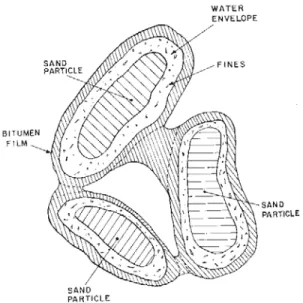
Oil sands are naturally viscous mixtures of sand or clay, water and an extremely heavy substance called bitumen (Figure 1.1). Bitumen is defined as “a thick, sticky form of crude oil” which is very heavy and viscous. Bitumen will not flow unless it’s heated or diluted with lighter hydrocarbons. At room temperature, it acts much like cold molasses. [1-2]. It can contain large amounts of sulfur and is the oil component of oil sands. Oil sands are also often referred to as tar sands or bituminous sand.

Each grain of sand is covered by a film of water, which is then surrounded by a slick of heavy oil (bitumen). The sands are bonded firmly together by grain-to-grain contact. The sand is composed of 92% quartz with traces of mica, rutile, zircon, tourmaline, titanium, nickel, iron, vanadium and

(17)

pyrite. The sand is triangular in shape, making it very abrasive. On the Moh’s hardness scale, with diamond being 10, oil sand is 7.4 [3]. The composition of oil sands is depicted in Figure 1.2.

Figure 1-1: Oil sands contain bitumen naturally

Figure 1-2: Composition of oil sands

Oil sand is often incorrectly referred to as “tar sand”, because the bitumen (or oil) resembles black, sticky tar. However, the term “oil sand” is the correct term. Tar is a man-made substance formed through the distillation of organic material. It is bitumen (a heavy thick oil), not tar, that

(18)

is found in the oil sands. The bitumen content in deposits varies from 1% – 18%. More than 12% bitumen content is considered rich, and less than 6% is poor and not usually considered economically feasible to mine, although it may be mined with a blended stock of higher grade oil sand. On average, it takes 2 tonnes of mined oil sand to produce one barrel of synthetic crude oil (159 litres). In the winter the water layer in the oil sand will freeze making it as hard as cured concrete. In the summer, it’s as soft as molasses making driving conditions treacherous [3].

Bitumen molecules contain thousands of carbon atoms. This makes bitumen one of the most complex molecules found in nature. In its natural state, it is not recoverable through a well like conventional petroleum. Bitumen cannot be refined into common petroleum products like gasoline, kerosene, or gas oil without first being upgraded to crude oil.

On average, bitumen is composed of: Carbon 83.2%

Hydrogen 10.4% Oxygen 0.94% Nitrogen 0.36% Sulphur 4.8%

Bitumen can be rich in either the hydrocarbons of the naphthalene type (used in making gasoline and petrochemicals), or asphaltenes type (used to make asphalt), depending on the type of fraction.

1.2.2 Oil sand deposits in Alberta

Alberta contains the largest concentration of oil sands in the world. The oil sands underlie 140,800 kilometres, or 21% of the province of Alberta. The mining portion of this land base will be approximately 4,750 square kilometres and that 99% of the mineable area has already been leased (Figure 1.3) [2]. Alberta’s oil sands are contained in three deposits: Athabasca, Cold Lake and Peace River (Figure 1.4) [3]. They cover an area the size of the province of New Brunswick in Canada or state of Florida in the United States. The entire area composes the largest single deposit of oil in the world, containing between 1.7 and 2.5 trillion barrels [1-4].

(19)

Figure 1-3: Land has been leased to oil sands mining operations, such as Suncor and Syncrude. Photo: David Dodge, The Pembina Institute [2]

Figure 1-4: Alberta’s three major oil sands areas: Athabasca, Cold Lake, and Peace River [3]

1.2.3 Formation of oil sand

It is believed that the oil sands were formed many millions of years ago when Alberta was covered by a warm tropical sea. The oil was formed in southern Alberta when tiny marine creatures died and fell to the bottom of the sea. Through pressure, heat and time, their tiny bodies were squished into the form of ooze which today we call petroleum (rock oil). In northern

(20)

Alberta, many rivers flowed away from the sea and deposited sand and sediment. When the Rocky Mountains formed, it put pressure on the land, and the oil, being a liquid, was squeezed northward and seeped into the sand, forming the Athabasca oil sands [3].

1.2.4 Oil sand recovery

Oil sands can be produced either through surfacing mining or in-situ methods which is the typical approach when the oil sands are too deep to support surface mining operations economically [1-3]. Surface-mining techniques require the removal of forest and layers of overburden (muskeg and topsoil) to expose the oil sands. Huge hydraulic power shovels dig into the oil sand and dump it into 400-ton heavy hauler trucks. The trucks transport the oil sand to a crusher unit that breaks it up, and then moves it by conveyor to the extraction plant. Previous mining methods included using a bucket-wheel, dragline, and conveyor system that was eventually phased out by 2006 [3].

1.2.5 Extracting the oil from the oil sand

Once mined, bitumen is separated from the sand using a hot water extraction process that was patented in the 1920s by Dr. Karl A. Clark [3]. Oil sand is mixed with hot water to form slurry (a very thick liquid) which is pipelined to a separation vessel. This is called hydro-transport. In the vessel, the slurry separates into three distinct layers: sand settles on the bottom, middlings (sand, clay and water) sit in the middle, and a thin layer of bitumen froth floats on the surface. The bitumen froth is skimmed off and spun in centrifuges to remove the remaining sand and water, and then goes to the upgrading plant. The leftover sand, clay, and water are pumped to large storage areas called tailings ponds or settling basins, and the water is recycled back into the extraction plant for re-use.

In the upgrading process, bitumen is chemically and physically changed into lighter products that can be easily refined. The two upgrading methods that are currently used are coking and hydro-treating. During coking, bitumen is heated to 500°C to break its complex hydrocarbon molecule into solid carbon called coke (which is very similar to coal) and various gas vapours. The gases are funnelled into a Fractionation Tower to be condensed and distilled into liquid gas oils that form synthetic crude oil. In the hydro-treating process, hydrogen is added to the bitumen to bond with the carbon in the molecule, creating more products while also removing impurities.

(21)

Only 20 percent of Alberta’s oil sands can be recovered through surface-mining techniques. If the oil sand layer is deeper than 75 metres from the surface, an in-situ technology is used. Steam Assisted Gravity Drainage (SAGD), is the most common in-situ process presently used. This process involves drilling two L-shaped wells parallel to each other into the deposit and injecting steam down through the top well. This warms the oil sand, and causes the bitumen to separate and flow downwards (using gravity) into the bottom well. It is then pumped to the surface for processing. Other in-situ methods include: Toe to Heal Air Injection (THAI), Vapour Extraction (VAPEX) and Cyclic Steam Stimulation.

1.2.6 Effect to the natural environment and economic importance for Canada

The impact on the natural environment is a major concern for mining companies. After mining, the land is reclaimed to its natural, productive state by using the left over sand (tailings sand), soil, overburden and muskeg that were originally there. Process water is stored in tailings ponds or settling basins on the mine site and re-used in the extraction process [3-4].

While current heavy oil production is only about 8 million bbl/d, between 500 and 1,000 billion bbl are considered recoverable with today’s technology and prices. In Canada, the Alberta Energy Resources Conservation Board estimates Alberta’s in-place oil sands reserves at 1.7 trillion bbl [1]. More than 175 billion bbl amount are recoverable with current technology [2-4]; with technical advances, 335 billion bbl could be recovered [4]. By 2015, oil sands production is expected to reach 3 million bbl/d. At current production rates, it would take 400 years to deplete the reserves at existing oil sands operations [4].

According to Alberta Energy Research Institute (AERI), there is a risk that the CO2 issue will have a significant negative impact on future oil sands development. AERI’s key strategies for developing next-generation oil sands technologies involve adding value by producing refined products and petrochemicals; reducing CO2 emissions, water use, natural gas use; and improving energy security.

1.2.7 Some economical-statistical information on oil sands in Canada

• For the period 1996-2016, approximately $87 billion of investment in oil sands development has been announced.

(22)

• Of the 63 oil sands projects under the generic royalty regime, 33 are in pre-payout (1%) while 30 are in post-payout (25%).

• Operating costs to produce a barrel of oil from bitumen averaged about $18 in 2004.

• Value-added upgrading of Alberta’s energy resources is a priority for the Alberta government. • Oil sand from the Athabasca area contains 83% sand, 3% clay, 4% water, and 10% bitumen. • It takes about two tonnes of oil sand to produce a barrel of oil.

• Oil sands producers move enough products (overburden and oil sands) every two days to fill Toronto’s Skydome or New York’s Yankee Stadium.

• Alberta’s 174 billion barrels of remaining established oil sands is enough oil to fill over 9 million Olympic size swimming pools.

• It takes 3 days oil to reach Edmonton via pipeline from the oil sands region. • Nine percent of U.S. crude imports are supplied by Canada.

• 93 % of oil sands reserves are designated as in-situ.

• 1,600,000 barrels of Canadian crude oil are exported to the United States daily. • 2,700,000 barrels of crude oil are produced daily.

1.3 Studies on oil sands

The first and only study of oil sands, that has inspired our final project in this study, was carried out by Bosisio et al [5]. In this experimental study, oil sand samples were heated with microwave power at a frequency of 2450±50 MHz. The incident power level was 100 W and it was possible to extract up to 86% of bitumen in oil sand test sample. It was a promising test study with a high extraction ratio in comparison with 70%, which is the highest extraction percentage by hot water and other thermal methods. This experimental reactor produced a crude oil called microwave crude oil (MCO) which is very similar to synthetic crude oil (SCO) and natural crude oil (NCO). This process of extracting oil from bitumen requires no water and therefore is much more environmental friendly.

Bosisio’s system, which worked at a frequency of 2450±50 MHz, encouraged us to develop a microwave energy applicator in order to extract bitumen in the tar sands with high level

(23)

microwave power. Our final research would be realized particularly at 2.45 GHz in order to separate crude oil from oil sands. The power would also be applied at up to 10,000 W which is much higher than Bosisio’s first experimental study using 100 W. The use of more than one low-level power source adds complexity and should be tested in order to reduce the cost of using one very expensive high-level microwave source.

For the first step of this proposed project, the behavior of the system at these frequencies such as complex permittivity of the oil sands should have been known. Related data in the literature for electrical properties of oil sands is very limited to develop a microwave energy applicator. When Akyel worked on reel time complex permittivity measurement, he measured some liquid materials obtained from oil including bitumen mixture by his reel-time system at 2.23 GHz [6]. In Sowa’s study [7], εr' and εr" value of water-in-bitumen emulsions were measured for the frequency range of 1 MHz and 10 MHz. Fauchard et al [8] studied electrical properties (including permittivity) of bitumen mixture component at 1.03 GHz, 1.7 GHz and 2.03 GHz. The only study on the complex permittivity measurement of the oil sands at 2450 MHz by using rectangular cavity resonator system was carried out by Erdogan et al [9-11] in the High Power Microwave Laboratory at École Polytechnique de Montréal. Since there was no data found in the literature for electrical properties of oil sands at ISM 2.45 GHz frequency (The Industrial, Scientific and Medical radio bands) until their measurement and reports were published, these data would be useful to continue designing and developing a microwave energy applicator to extract bitumen from oil sands. This memoire builds on the study details reported by Erdogan et al [9-11].

(24)

CHAPTER 2 EXPERIMENTAL DETAILS

2.1 Complex permittivity

Microwave energy has been applied in many fields such as agriculture, food, microwave-assisted chemistry, communication, medical treatments, bioengineering, and construction industry. In recent years, enormous demands and ideas have grown in the application of microwave energy to the processing of a large variety of new and engineered materials. Microwave energy provides an efficient and clean heating process compared to conventional processing methods with wide a range of temperatures (2000° C or more). Principally, microwave energy heating is different from conventional energy heating since electromagnetic energy is directly transferred to the material and absorbed by the material. Microwave energy penetrates and produces heat directly within the material and thus provides energy savings.

Permittivity or in general complex permittivity of a material describes how a material reacts to an electric field and how the material store and dissipate the energy after being exposed to electromagnetic energy. Materials can be electromagnetically characterized by three main parameters: conductivity (σ in S/m), permittivity (ε in F/m), and permeability (µ in H/m). In a linear, homogeneous and isotropic medium, the electromagnetic fields are related to these parameters by the relations of:

H B (2.1) E J  (2.2) E D  (2.3)

where the magnetic flux density B (Wb/m2) is proportional to the strength of the magnetic field H (A/m) through permeability, the current density J (A/ m2) is proportional to the strength of the electric field E (V/m) through the conductivity and the displacement field D (C/m2) is proportional to the strength of the electric field E (V/m) through permittivity.

Microwave engineering requires precise knowledge of electromagnetic properties, particularly dielectric properties of materials at microwave frequencies [12] since the successful application of microwaves is directly associated with the dielectric properties of the materials. These

(25)

properties are defined in terms of dielectric constant (ε') and loss factor (ε") [13]. The word dielectric was used for the first time by Faraday [14]. A dielectric is a non-conducting substance, i.e. an insulator whose permittivity:

 

   j (2.4) 

Permittivity is actually a complex number. In engineering, it is very common to use permittivity in terms of its relation to permittivity of free space:

0

. 

  _r (2.5)

where ε0 is the permittivity of free space, 8.8541887817x10-12.

Throughout our presentation, the term permittivity is considered and used in terms of its relative value as opposed to its absolute value.

The relative complex permittivity (i.e. dielectric constant) is also complex when the permittivity is complex and it is the ratio of epsilon complex to epsilon zero [15]:

r r r j j _ _               0 0 . (2.6)

Both the real (εr') and the imaginary part (εr") of the relative complex dielectric constant (εr = εr' - jεr") can be measured by using cavity perturbation technique.

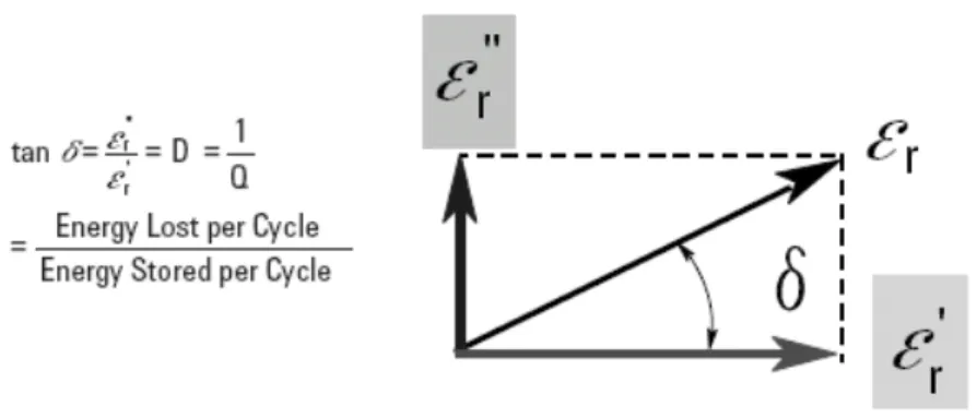
Another important parameter related to permittivity is the loss tangent (tanδ) which describes electromagnetic characterization of materials. The loss tangent it the ratio of the amount of energy lost in a material to the amount of energy stored in a material as depicted in Figure 2.1. In engineering, loss tangent is widely used as opposed to loss factor. It can be written explicitly as:

      tan . (2.7)

The measurement of electromagnetic parameters of the dielectric and insulating materials has been studied since they were used to store electrical energy. Dielectric materials are essential for manufacturing electronic components such as circuit boards, electronic lumped components used in circuits and antennas, etc. Designers and engineers must calculate harness level of electrical energy when the material plays an important role in the design.

(26)

Figure 2-1: The real part (εr') and the imaginary part (εr") of complex permittivity

In 1800, liquid dielectrics were the first application of insulators for transformers and as fillers for high voltage cables [16]. Recent applications, mostly in chemical, food or biomedical industries, require a combination of pure liquids, as well as mixtures, emulsions and colloids. Further developments and applications with pure and mixture liquid dielectric materials have brought a high demand for the permittivity measurement of these materials.

Dielectrics can be usefully classified into different categories depending on either application or measurement method. Geyer [17] classified materials in terms of their dielectric characteristics:

 Low dielectric constant, low loss (εr' ≥ 4, tanδ < 0.001)  High dielectric constant, low loss (εr' ≥ 10, tanδ < 0.001)

 Very high dielectric constant, ultra-low loss (εr' ≥ 100, tanδ < 0.0002)  Lossy dielectric (tanδ ≥ 0.1)

2.2 Experimental setup: microwave cavity perturbation technique

There are many techniques for permittivity measurement at microwave frequencies. The transmission/reflection technique, the open-ended coaxial probe technique, the cavity perturbation technique and time-domain spectroscopy technique are the most common measurement techniques for liquid or semi-solid materials [18 - 20]. The cavity perturbation method has several advantages compared to other permittivity measurement techniques. In general, it is the most accurate technique for measuring very low-loss dielectrics. The main difference with the coaxial probe technique is that the cavity perturbation technique does not

(27)

need calibration to perform or maintain valid measurements. It may require specific machining to locate the sample in the cavity, but it does not require as much material as other techniques. The earliest treatment of cavity-perturbation theory was studied by Bethe and Schwinger [21]. A method was presented by Von Hippel to determine the complex permittivity from the reflection coefficient of the TE1,0 mode in a rectangular waveguide [22]. Many researchers [23 - 32] have studied and employed Bethe and Schwinger’s cavity-perturbation method in order to measure the conductivity and the dielectric constant of materials at microwave frequencies.

The cavity construction is simple. It is possible to get experimental data at several discrete frequencies covering the whole frequency band [27]. When a small material sample is inserted into a resonant cavity, it will cause a complex frequency shift [31]. The most practical means of developing a high frequency (high Q resonator) is to enclose the fields within a body whose dimensions are comparable to the desired wavelength of operation. Such a device is normally referred to as a resonant cavity, and will support a series of modes, with a lower cut-off, each corresponding to a unique distribution of fields. For ease of fabrication, one is generally limited to cylindrical or rectangular cavities, and in these cases one can easily determine the field distribution within the resonator.

2.2.1 Rectangular cavity with the structure of a rectangular waveguide

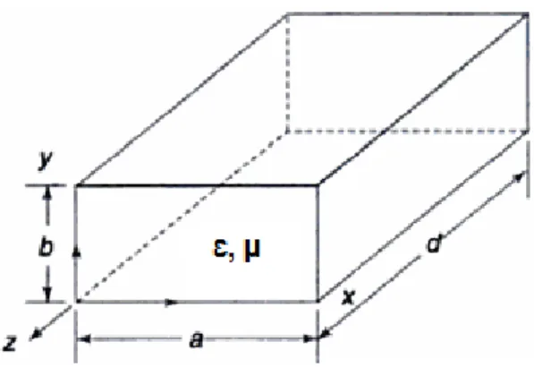
Rectangular waveguides are one of the earliest types of transmission lines. They have many applications. A rectangular waveguide can support TM and TE modes, but not TEM waves, because it is not possible to define a unique voltage since there is only one conductor in a rectangular waveguide. A rectangular waveguide with dimensions d (length), a (width) and b (height) cannot propagate below a certain frequency (assuming d>a>b). This frequency (fc) is called the cut-off frequency in the waveguide.

As seen in Figure 2.2, a rectangular cavity may be a section of a rectangular waveguide terminated by a short circuit at one end in the z-direction (z=d). If d equals a multiple of a half guide-wavelength at the frequency of f, the resulting standing-wave pattern is such that the x and y components of the electric field are zero at z=0. Consequently, a short circuit can be placed at the beginning of the z-direction (z=0) as well. The resulting structure considered a rectangular cavity [33].

(28)

Figure 2-2: Rectangular cavity perspective view

TEm,n modes (Ez=0 and Hz≠0) exist in a rectangular waveguide. Similarly, in a rectangular cavity, there are TEm,n,p modes (Ez=0 and Hz≠0) and we can measure the resonant frequency (fr) instead of the cut-off frequency (fc). In TEm,n,p modes, the resonant frequency (fr) of a rectangular cavity can be written as:

) ( 2 1 2 2 2 Hz d p b n a m f_r                       . (2.8)

where m, n and p represent possible modes and 1/  is the wave propagation speed in the guide. It is shown as the TEm,n,p mode for the cavity. Here, m denotes the number of half cycle variations of the fields in the x-direction (“a” direction), n denotes the number of half cycle variations of the fields in the y-direction (“b” direction) and p denotes the number of half cycle variations of the fields in the z-direction (“d” direction).

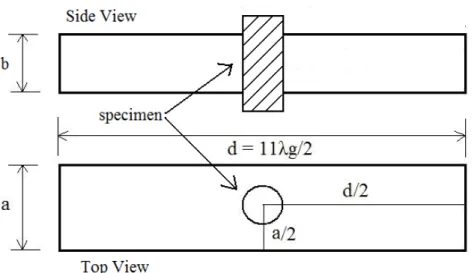
For a rectangular cavity, the TE1,0,p mode (p is an integer) is widely used for to measure complex permittivity.The sample is placed in the position of maximum electric field. Usually there are p positions in the cavity with maximum electric field for the TE1,0,p modes. When p is an odd number, the position of maximum electric field is in the middle of the cavity (geometrical center) for the TE1,0,p mode despite the fact that the maximum field positions change with changing p values as illustrated in Figure 2.3. This makes measurement easier since there is no need to calculate the position of maximum electric field in the cavity [34].

(29)

Figure 2-3: TE rectangular cavity side and top views for cavity perturbation technique (the a, b, and d are the width, height, and length of the cavity, respectively)

Complex permittivity is calculated from changes in the resonant frequency (fr) and the quality factor (Q). For this study, the mode has been determined TE1,0,11 which is one half cycle of a field variation in the x-direction and eleven half cycle of a field variation in the z-direction. For TE1,0,11 mode, (2.8) can be simplified for air-filled rectangular cavity as:

 

1 11 ( ) 2 2 2 11 , 0 , 1 _a _d Hz c f_r               (2.9)

where c is the speed of the light in free space.

We need to calculate Q values for the empty cavity and sample loaded cavity. The changes of f and Q of the cavity [34 - 35] can be expressed as







          0 2 1 2 1 0 ₁ 2 V V s s dV E dV E E f f f  s _, (2.10)



   0 2 1 2 1 0 1 1 V V s E dV dV E E Q Q s  (2.11)

(30)

where f0 and fs are the resonant frequencies of the empty cavity and the sample loaded cavity respectively, Q0 and Qs are the measured quality factors of the cavity without and with a lossy sample inside the cavity, V0 and Vs are the volume of empty cavity and the volume of sample, and E1 and E2 are the electric fields in the empty cavity and sample loaded cavity.

As mentioned above, the basic assumption for the cavity perturbation technique, which was studied by Bethe-Schwinger [21] and Von Hippel [22], is that the change of electromagnetic field upon the introduction of the sample must be small. From this assumption, inserting the sample symmetrically into the region of maximum electric field, according to Dube [28, 35] and Verna [35], the real and imaginary parts of the relative complex permittivity are calculated by:





₁ 2 0 0  _   s s s f V f f V  , (2.12)          0 0 1 1 4V Q Q V s s  . (2.13)

According to Akyel [6], the measured Q values (Q0 and Qs) of the cavity are calculated as:

) 3 ( ) 3 ( 3 f dB f dB f f f Q L R dB resonant     . (2.14)

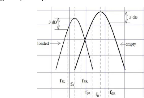
Figure 2-4: The graphs of the vector network analyzer of Q factors for the empty cavity and the sample loaded cavity when permittivity is measured using the cavity perturbation techniques (f0=the resonant frequency of the empty cavity, fs=the resonant frequency of the loaded cavity)

(31)

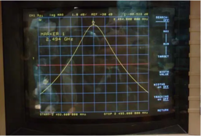
In (2.14), the resonant frequency f (peak S21 value on VNA-Vector Network Analyzer) and the half power bandwidth Δf3dB will be read on VNA for both the empty cavity and the sample loaded cavity as illustrated in Figure 2.4 and its screen picture on VNA is shown in Figure 2.5.

Figure 2-5: Screen picture of Q factors on a Vector Network Analyzer (VNA)

2.2.2 Interactions of electromagnetic wave with lossy dielectrics and energy

loss

According to Puschner [36], when we study dielectric materials, we observe the reactions which take place between an alternating electric field E and the atomic and molecular elements of the dielectric. The effective losses which appear as heat through these reactions in the dielectric are of interest to the practising engineer. With frequencies above 1000 MHz, it is usual to interpret the energy processes with the help of electromagnetic waves. The propagation energy of the electromagnetic wave can be deduced from Maxwell equations and leads to Poynting’s theorem. If we assume an approximately homogeneous electric field in the volume, necessary dissipation in the dielectric can be written as:

 

_ _          3 2 2 12 10 556 . 0 m W Hz f m V E P_loss _r . (2.15)

The energy converted into heat by the alternating electric field increases according to (2.15) in proportion to the frequency and the square of the electric field strength. The rise in the field strength is restricted by the finite dielectric strength of the dielectric so that the specific energy

(32)

conversion can only be raised by increasing the frequency. This is the essence of microwave heating. In general, Puschner [36] explains that the loss factor rises with increasing frequency. Even with falling values, the increase in the specific energy conversion according to (2.15) is very much greater when the frequency is raised.

2.2.3 Advantages and disadvantages of the rectangular cavity perturbation

technique

The cavity perturbation technique has many advantages to measure complex permittivity. First of all, the rectangular cavity is easy to design and build. The required hardware does not require very precise machining or special material. For our study, the rectangular resonator was made of copper with two loop antennas at each ends for excitation by Vector Network Analyzer (VNA). The cavity perturbation is the most accurate method for measuring low-loss materials. This advantage makes it very suitable for determining the complex permittivity of oil sand since it is expected a low-loss dielectric material. Unlike some other techniques, such as the coaxial probe technique, there is no need for calibration to perform or maintain valid measurements.

The main disadvantage of the cavity perturbation technique is determining the dielectric constant and conductivity at either one single frequency, or at a narrow band of frequencies. The measurement setup of the cavity is not practical and it is not easy to construct for many distinct frequencies or wide band measurement. This disadvantage was not an issue for our study since it was carried at only at 2.45 GHz, an ISM frequency (The Industrial, Scientific and Medical radio bands which are defined by the ITU-R in 5.138, 5.150, and 5.280 of the Radio Regulations). Sample is assumed to be homogeneous and isotropic. Although most liquids and semi-solid materials are homogenous (making this technique very suitable for determining their complex permittivity), unfortunately, oil sand cannot be classified as purely homogeneous because oil sand may contain different sized aggregates and different levels of humidity. During the measurements in the laboratory, we prepared the samples homogeneously as possible, but samples from different locations of the Alberta oil sands might cause slightly different values to be measured.

Due to geometrical design and sample placement problems, in some cavity shapes the samples may require very specific machining to fit into the cavity. In our study, a hole at the top and a

(33)

hole at the bottom were opened to insert a cylindrical glass sample holder containing the sample. Therefore, this disadvantage was not an issue for our study.

The volume of the sample must be small comparing to the volume of the cavity used. If the volume of the sample is very small may cause very small change in the Q factor and in frequency to be measured. Ideally, the sample must be small enough for the fields in the cavity. The physical size of the resonator itself is also a factor to consider for determining the ideal sample type. While large resonators provide a much higher unperturbed Q factor, a too large resonator may reduce the overall effectiveness of the measurement. In our study, length of cavity was taken long enough (11λg/2, eleven half cycles in the waveguide) to reach small ratio of sample volume to waveguide volume. Thus, the design of cavity resonator was able to satisfy the assumptions made for the perturbation theory and approximation.

One important drawback with the cavity perturbation technique is other undesired modes within the cavity due to the resonant leakages. Any kind connector interface may cause a non-resonant coupling between input and output port that will decrease the overall energy storage of the instrument. By designing the cavity long enough helped the separate modes and allowed to work at TE1,0,11 mode without interfering in other modes.

One small source of error for this method is the leakage from the holes at the bottom and the top of the cavity (Figure 2.3) which are necessary to insert sample into the resonator. The magnetic fields around the hole (with or without samples) impact the assumptions of the perturbation theory and affect the accuracy of the measurements.

Another drawback of this technique is to read the values on the VNA. The information in the resonant frequency and the Q factor are obtained via signal amplitude measurements at the peak and -3 dB points. Such amplitude measurements are inaccurate due to the difficulty in obtaining perfect matching in the transmission system. In addition, low Q values of cavities containing lossy materials increase the difficulty of determining the exact frequencies at which the peak and -3 dB amplitude points occur [25].

Carter found in his study that cavity perturbation technique might have up to 5% the measurement errors for rod-type sample inserted into the resonator [37].

(34)

CHAPTER 3 MEASUREMENTS

3.1 Design and constructing of a rectangular cavity resonator for our study

This study presents a rectangular cavity whose upper view of the rectangular cavity waveguide (depicted in Figure 3) was designed and constructed at École Polytechnique de Montréal laboratories. A standard waveguide made of copper was chosen with the width of 72.2 mm and the height of 34.1 mm.

The calculations for the cavity such as cut-off frequency of waveguide were based on TE1,0 mode since the TE1,0 mode is the dominant mode in a rectangular waveguide. The ideal rectangular cavity resonant frequency in the air for TE1,0,11 mode was 2.45 GHz, as shown in (2.8). However, the actual working (resonant) frequency for TE1,0,11 mode in our study was 2.49 GHz due to the frequency shift factor when the sample loaded. This frequency is still valid. In ISM radio bands, one of the frequency ranges is between 2.400 and 2.500 GHz.

Since oil sand is expected to behave as a low-loss dielectric material, the oil sand sample volume should be higher than other high-loss dielectric liquids. However, the volume of the cavity had to be much higher than usual in order to maintain a very small ratio of sample volume to cavity volume. To provide this, the length of the cavity, shown in Figure 3.1, was chosen as 11λg/2 (1186.55 mm) where λg is the wavelength in the waveguide. Choosing a long waveguide also has the advantage of separating the modes enough in the resonator.

After determining the mode (TE1,0 for waveguide and TE1,0,11 for cavity resonator) and the dimensions of the cavity resonator, the cut-off frequency fc was calculated as 2.077 GHz, the wavelength in the air λ0 as 120.00 mm, and the wavelength in the guide λg as 215.14 mm. The length of the entire waveguide, which was equal to 11λg/2, is 1186.55 mm. The rectangular cavity resonator fabricated for our study during the measurements is shown in Figure 3.1.

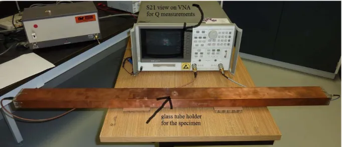
Waveguide resonator had two loop antennas at both ends for excitation from a Vector Network Analyzer (VNA). A hole at the top and a hole at the bottom were drilled to insert a cylindrical glass tube holder containing the sample. The diameter of the holes was 6.12 mm and it perfectly held the glass sample holder (a rod) in a cylindrical geometry with a diameter of 6.1 mm. The length of the glass tube holder was longer than the height of waveguide (dimension b) in order to fit the sampler perfectly into the holes.

(35)

Figure 3-1: The cavity resonator built for our study at École Polytechnique de Montréal laboratories (the length of 1186.55 mm, and made of copper)

The volume of the oil sands in the glass tube holder was around 990 mm3. This volume was enough to induce a measurable change in the Q factors and resonant frequencies. The Sampling volume of other well-known liquids was reduced to around 15-25 mm3 for the verification purposes since their dielectric loss values are higher than bitumen of oil sands (see section 3.3). In the resonant cavity technique, the volume of the sample must be as small as possible so that measurements will be as accurate as possible.

3.2 Measurement process

The rectangular cavity resonator was excited with VNA at both ends through small loop antennas. The empty cavity with empty glass tube holder in the hole was first excited to find its resonant frequency and Q factor of empty cavity. Then, the glass tube holder was taken out, filled up with the sample and put back to the hole. The sample loaded cavity was excited again to find its shifted resonant frequency and Q factor. If the field for the cavity can be explicitly determined, then these two parameters can be used to calculate complex permittivity values of the sample material as given in (2.12) and (2.13).

(36)

3.3 Measurement values

The Bitumen from oil sand samples obtained from Alberta oil sand resources were classified into very low, low and high grade samples (the oilier bitumen is considered the higher grade). Measurement results were repeatable after some practical problems and errors caused by the experiment setup were solved. The oil sand sample measurements by our in-house designed and manufactured rectangular cavity resonator are shown in the first three lines of the Table 3.1.

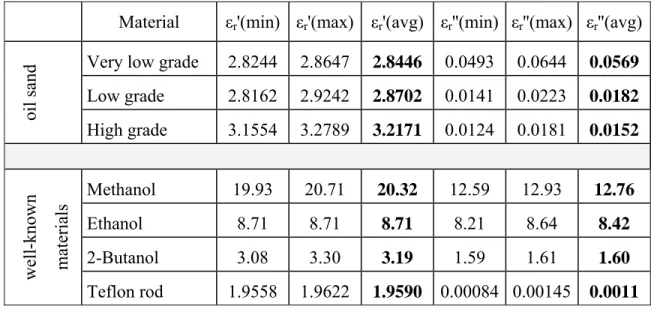
Table 3.1: Measurement values obtained by in-house rectangular cavity resonator Material εr'(min) εr'(max) εr'(avg) εr''(min) εr''(max) εr''(avg)

oil sand

Very low grade 2.8244 2.8647 2.8446 0.0493 0.0644 0.0569 Low grade 2.8162 2.9242 2.8702 0.0141 0.0223 0.0182 High grade 3.1554 3.2789 3.2171 0.0124 0.0181 0.0152 well-known mate ria ls Methanol 19.93 20.71 20.32 12.59 12.93 12.76 Ethanol 8.71 8.71 8.71 8.21 8.64 8.42 2-Butanol 3.08 3.30 3.19 1.59 1.61 1.60 Teflon rod 1.9558 1.9622 1.9590 0.00084 0.00145 0.0011

Some well-known liquids such as ethanol, methanol and 2-butanol, and a well-known solid such as a Teflon rod were also measured for verification and their values are also presented in the last four lines of the Table 3.1.

All the results in Table 3.1 show the minimum and maximum values of εr' and εr'' of the materials measured at the temperature of 23° C and at the frequency of 2.49 GHz.

3.4 Verification process

It can be assumed that the values of oil sand samples measured by 11λg/2-length rectangular cavity are correct and can be used as reliable values if the values of well-known substances are

(37)

comparable to the values measured by a commercial system or the values found in the literature. Verification was carried out in two ways:

3.4.1 Our study measurements compared to another system

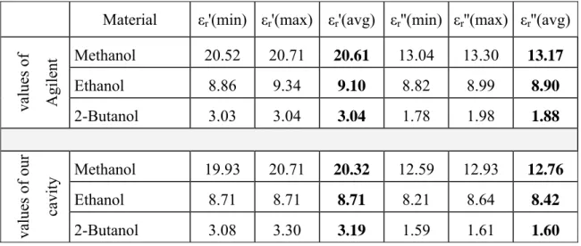
Throughout the study, the well-known substances (methanol, ethanol and 2-buthanol) were first measured by rectangular cavity with the length of 11λg/2 which was manufactured in our laboratory. Then the same substances were measured by a commercial system called Agilent 85070 slim form probe using an open-ended coaxial probe technique. Table 3.2 shows the results of the measurements (values of εr' and εr'') carried out by the Agilent 85070 probe system which was calibrated by open circuit, short circuit and air. The measurements and calibration were performed exactly at the same temperature (23°C) and at the frequency (2.49 GHz) as the rectangular cavity resonator.

Table 3.2: Measurement values obtained by Agilent 85070 slim form probe

Material εr'(min) εr'(max) εr'(avg) εr''(min) εr''(max) εr''(avg)

values of Agilent Methanol 20.52 20.71 20.61 13.04 13.30 13.17 Ethanol 8.86 9.34 9.10 8.82 8.99 8.90 2-Butanol 3.03 3.04 3.04 1.78 1.98 1.88 values of our cavity Methanol 19.93 20.71 20.32 12.59 12.93 12.76 Ethanol 8.71 8.71 8.71 8.21 8.64 8.42 2-Butanol 3.08 3.30 3.19 1.59 1.61 1.60

3.4.2 Our study measurements compared to the values in the literature

The values of the well-known liquid substances obtained by our in-house cavity were also compared with some similar values found in the literature as shown in Table 3.3. The in-house Teflon rod measurement was only compared to the values found in literature because the Agilent 85070 probe is not suitable for measuring solids or semi-solid substances.

(38)

Table 3.3: The values of the well-known substances found in the literature

Material εr' εr'' Source f (GHz) T (° C)

Methanol 20.32 12.76 our study 2.49 23

22 14 Jordan [39] 2.49 20

22.5 13.0 Ghannouchi [40] 2.49 25

21 13 Anderson [38] 2.49 20

Ethanol 8.71 8.42 our study 2.49 23

8.3 8.2 Lane [41] 2.49 25

7.7 6.9 Ghannouchi [40] 2.49 25

8.2 9.0 Anderson [38] 2.49 20

2-Butanol 3.19 1.60 our study 2.49 23

3.7 1.65 Von Hippel [42] 3.00 25 Teflon rod 1.9590 0.0011 our study 2.49 23

1.95 0.001 Akyel [6] 2.0 27

Table 3.3 compares our study values of the complex permittivity values of the well-known substances to the values found in the literature at the closest frequency to our study (2.49 GHz) and at the closest temperature to our study (23 °C). The values found in the literature might have been obtained by different techniques than rectangular cavity resonator.

(39)

CHAPTER 4 DISCUSSION AND CONCLUSION

4.1 Comparison of the permittivity measurements of liquid substances

The results of the methanol, ethanol and 2-butanol measurements obtained through our in-house resonator (Table 3.1) and the Agilent 85070 slim form probe (Table 3.2) have an excellent matching at the same resonant frequency and temperature for both values of εr' and εr''. They are in 5% error range.

For methanol and ethanol, the differences between our measurement (Table 3.1) and the results found in the literature (Table 3.3) seem to be slightly higher than 5% error range. This is expected since the results found in the literature were obtained at different frequencies and/or different temperatures. The complex permittivity values of very lossy substances such as methanol and ethanol vary with frequency and temperature.

For 2-butanol, we observed a quasi perfect agreement (particularly for εr'') between our result (Table 3.1) and the result found by Von Hippel (Table 3.3) although the temperature and frequency are slightly different. This is expected since 2-butanol can be considered as a low-loss substance compared to methanol and ethanol.

The cavity resonator technique used in our study is very suitable for low-loss materials. Among the substances used for comparison, 2-butanol is the most reliable substance for our study since it is in liquid form and has low-loss dielectric properties like bitumen in oil sand.

In conclusion, based on comparison to the Agilent 85070 probe, we can rely on the measurements from our in-house resonator because the measurements were carried out under the same conditions (at the same time, at the same frequency and with the same samples) for the methanol, ethanol and 2-butanol measurements.

4.2 Comparison of the Teflon measurement

Since Teflon is a solid, it was not possible to measure its complex permittivity with the Agilent 85070 slim form probe. The Teflon measurement obtained through in-house resonator (Table 3.1) is compared only to a result found by Akyel [6] in which the temperature and frequency are slightly different. In the literature, some researchers found the values of εr' to be around 2.0 and 2.05 for Teflon at a different frequency or temperature. This is very close to our measurement of

(40)

1.95. This is an expected result since Teflon is known as a very low-loss substance and the cavity resonator technique used in our study is very suitable for low-loss material. Among the substances that the complex permittivity values were measured for comparison, Teflon is another reliable substance as 2-butanol because Teflon has also low-loss dielectric properties although its solid form is not the same as oil sand.

In closing, a good agreement is obtained between the Agilent probe measurements and the cavity based measurements for the same testing conditions (temperature, frequency, materiel sample). In addition, the measurement of Teflon using the developed setup led to results that are in agreement with those found in the open literature. Therefore, our findings show that in-house rectangular cavity resonator is able to accurately measure the permittivity of oil sands. Our measurements for oil sands as shown in the Table 3.1 can be trusted as correct values.

4.3 Conclusion

In our study, we obtained the complex permittivity values of εr' and εr'' of oil sands by using the cavity perturbation technique at frequency of ISM 2.45 GHz with one mode (TE1,0,11). This technique has been widely used in the measurement of dielectric parameters of various materials. The advantage of this technique is that it is the most accurate method for measuring low-loss materials, making it very suitable for determining the complex permittivity of oil sands because oil sand a low-loss material. The samples required for the measurements in a rectangular cavity must be in the form of a rod with their heights equal at least to the height of the cavity to produce accurate measurements.

Our rectangular resonant cavity was designed and fabricated at École Polytechnique de Montréal laboratories. The oil sand samples were classified into three groups depending on their oil content: high, low or very low grade. Several measurements were carried out with oil sand samples as well as other well-known substances (methanol, ethanol, 2-butanol and Teflon) for the purpose of verification. The Liquids were also measured by a commercial system (Agilent 85070 slim form probe) under the same conditions. We had to use a value from the literature as a comparison for the Teflon measurement. As explained in the discussion section, our measurement values are very similar to comparison values particularly with the results obtained through the commercial system. Therefore, we may conclude that the results obtained through

(41)

our in-house cavity resonator are accurate and reliable complex permittivity values for the measuring oil sands from Alberta oil sand resources.

The ability to determine of complex permittivity values is very crucial to the design and implementation of a microwave energy applicator for processing oil sands and extracting bitumen from oil sand in a more cost efficient and environmental sound manner. Since there is no study in the literature about the complex permittivity values of oil sands at ISM 2.45 GHz, our study would be of a great help and an important guide for those who plan to design and manufacture microwave energy applicators in order to extract bitumen from the oil sands.

The oil sand measurement values in Table 3.1 show that complex permittivity values of oil sands are very low. It seems that a chemical reaction in the oil sand by heating it with low-level microwave energy is doubtful. After obtaining the measurements, in order to observe a reaction of oil sands against microwave, we applied almost 1900 W to the 100 grams of high grade sample in a microwave oven for a little over 15 minutes. We were not able to see any extraction or melting. Then, we mixed the oil sand sample with charcoal (containing 90% carbon) in order to accelerate the reaction. In the 100 gram mixture, there were 20 grams of charcoal and 80 grams of oil sand. We again applied almost 1900 W to the 100 gram mixture in a microwave oven for a little over 15 minutes. We observed some very limited melting due to high temperature, but no sign of extraction. This experiment shows that oil sands having low-level loss factor (εr'') cannot be heated at low level microwave energy.

This is not a conflict with Bosisio’s experimental studies [5] since he created plasma in the center of a cavity into which an oil sand sample was placed. He was able to apply a very high energy level to the sample thanks to plasma. This may be possible setting in a laboratory but unfortunately, in nature, where we intend to use microwave energy applicator, creating plasma is not a feasible process. In order to realize a microwave energy applicator to extract bitumen from oil sands, we would need to consider to applying very high power such as 10 KW or more. Otherwise we would search different frequencies at which oil sands show a higher loss factor against microwave, if possible.

(42)

BIBLIOGRAPHY

[1] Government of Alberta, “Alberta’s oil sands,” Government of Alberta, Alberta, March 2008, ISBN 978-07785-7348-7 [Online]. Available :

http://www.environment.alberta.ca/documents/Oil_Sands_Opportunity_Balance.pdf.

[2] Simon Dyer, “Environmental impacts of oil sands development in Alberta,” The Oil Drum, Alberta, September 2009 [Online]. Available:

http://www.theoildrum.com/pdf/theoildrum_5771.pdf.

[3] Oil Sand Discovery Centre, “Facts about Alberta’s oil sands and its industry,” Oil Sand Discovery Centre, Alberta, Facts Sheet, 2009 [Online]. Available: http://www.oilsandsdiscovery.com/oil_sands_story/pdfs/facts_sheets09.pdf.

[4] Alberta Energy, “Facts on oil sands,” Alberta Energy, Alberta, Facts Sheet, June 2006 [Online]. Available: http://www.energy.alberta.ca/OilSands/pdfs/FactSheet_OilSands.pdf. [5] R.G. Bosisio, J.L. Cambon, C. Chavarie and D. Klavana, “Experimental results on the heating of Athabasca tar sand samples with microwave power,” Journal of Microwave Power, 12(4), pp. 301-307, 1977.

[6] C. Akyel, “Système hyperfréquentiel de mesure et de calcul de la permittivité complexe en temps réel,” Ph.D., Department of Electrical Engineering, École Polytechnique de Montréal, QC, Canada, 1980.

[7] J.M. Sowa, P. Sheng, M. Y. Zhou, T. Chen, A.J. Serres and M.C. Sieben, “Electrical propeties of bitumen emulsions,” Fuel, vol74, no. 8 pp. 1176-1179, 1995.

[8] C. Fauchard et al, “Estimation of compaction of bituminous mixtures at microwave frequencies,” in Non-Destructive Testing in Civil Engineering Nantes-NDTCE-2009, France, 2009[Online]. Available: http://www.ndt.net/article/ndtce2009/papers/220.pdf.

[9] L. Erdogan, C. Akyel and F. M. Ghannouchi, “Dielectric properties of oil sands at 2.45 GHz with TE1,0,11 mode determined by a rectangular cavity resonator,” Journal of Microwave Power and Electromagnetic Energy, 45 (1), pp. 15-23, 2011 [Online]. Available: http://jmpee.org/jmpee_site/Vol_45/JMPEE45-1-15Erdogan.pdf.

Dielectric Properties of Oil Sands at 2.45 GHz Determined with Rectangular Cavity Resonator