Constraints on models for the Higgs boson with exotic spin and parity in VH→Vbb¯ final states

arXiv:1407.6369v2 [hep-ex] 8 Sep 2014

Constraints on models for the Higgs boson with exotic

spin and parity in V H → V b¯

b

_{final states}

V.M. Abazov,31_{B. Abbott,}67 _{B.S. Acharya,}25 _{M. Adams,}46 _{T. Adams,}44 _{J.P. Agnew,}41 _{G.D. Alexeev,}31

G. Alkhazov,35 _{A. Alton}a_,56 _{A. Askew,}44 _{S. Atkins,}54 _{K. Augsten,}7 _{C. Avila,}5 _{F. Badaud,}10 _{L. Bagby,}45

B. Baldin,45 _{D.V. Bandurin,}73_{S. Banerjee,}25 _{E. Barberis,}55 _{P. Baringer,}53_{J.F. Bartlett,}45 _{U. Bassler,}15

V. Bazterra,46 _{A. Bean,}53_{M. Begalli,}2 _{L. Bellantoni,}45 _{S.B. Beri,}23_{G. Bernardi,}14_{R. Bernhard,}19 _{I. Bertram,}39

M. Besan¸con,15 _{R. Beuselinck,}40 _{P.C. Bhat,}45 _{S. Bhatia,}58 _{V. Bhatnagar,}23 _{G. Blazey,}47 _{S. Blessing,}44_{K. Bloom,}59

A. Boehnlein,45 _{D. Boline,}64 _{E.E. Boos,}33 _{G. Borissov,}39_{M. Borysova}l_,38 _{A. Brandt,}70 _{O. Brandt,}20 _{R. Brock,}57

A. Bross,45 _{D. Brown,}14 _{X.B. Bu,}45 _{M. Buehler,}45_{V. Buescher,}21_{V. Bunichev,}33 _{S. Burdin}b_,39 _{C.P. Buszello,}37

E. Camacho-P´erez,28 _{B.C.K. Casey,}45 _{H. Castilla-Valdez,}28 _{S. Caughron,}57 _{S. Chakrabarti,}64 _{K.M. Chan,}51

A. Chandra,72 _{E. Chapon,}15_{G. Chen,}53 _{S.W. Cho,}27 _{S. Choi,}27 _{B. Choudhary,}24 _{S. Cihangir,}45 _{D. Claes,}59

J. Clutter,53 _{M. Cooke}k_,45 _{W.E. Cooper,}45 _{M. Corcoran,}72 _{F. Couderc,}15 _{M.-C. Cousinou,}12 _{D. Cutts,}69

A. Das,42 _{G. Davies,}40 _{S.J. de Jong,}29, 30 _{E. De La Cruz-Burelo,}28 _{F. D´eliot,}15 _{R. Demina,}63 _{D. Denisov,}45

S.P. Denisov,34 _{S. Desai,}45 _{C. Deterre}c_,20 _{K. DeVaughan,}59 _{H.T. Diehl,}45 _{M. Diesburg,}45 _{P.F. Ding,}41

A. Dominguez,59 _{A. Dubey,}24 _{L.V. Dudko,}33 _{A. Duperrin,}12 _{S. Dutt,}23 _{M. Eads,}47 _{D. Edmunds,}57

J. Ellison,43_{V.D. Elvira,}45 _{Y. Enari,}14_{H. Evans,}49 _{V.N. Evdokimov,}34_{A. Faur´e,}15 _{L. Feng,}47 _{T. Ferbel,}63

F. Fiedler,21 _{F. Filthaut,}29, 30 _{W. Fisher,}57 _{H.E. Fisk,}45 _{M. Fortner,}47 _{H. Fox,}39 _{S. Fuess,}45 _{P.H. Garbincius,}45

A. Garcia-Bellido,63_{J.A. Garc´ıa-Gonz´alez,}28 _{V. Gavrilov,}32 _{W. Geng,}12, 57 _{C.E. Gerber,}46 _{Y. Gershtein,}60

G. Ginther,45, 63 _{O. Gogota,}38_{G. Golovanov,}31 _{P.D. Grannis,}64 _{S. Greder,}16 _{H. Greenlee,}45 _{G. Grenier,}17

Ph. Gris,10_{J.-F. Grivaz,}13 _{A. Grohsjean}c_,15_{S. Gr¨unendahl,}45_{M.W. Gr¨unewald,}26 _{T. Guillemin,}13_{G. Gutierrez,}45

P. Gutierrez,67 _{J. Haley,}68 _{L. Han,}4 _{K. Harder,}41_{A. Harel,}63 _{J.M. Hauptman,}52 _{J. Hays,}40 _{T. Head,}41

T. Hebbeker,18 _{D. Hedin,}47 _{H. Hegab,}68 _{A.P. Heinson,}43 _{U. Heintz,}69 _{C. Hensel,}1 _{I. Heredia-De La Cruz}d_,28

K. Herner,45 _{G. Hesketh}f_,41_{M.D. Hildreth,}51 _{R. Hirosky,}73_{T. Hoang,}44_{J.D. Hobbs,}64 _{B. Hoeneisen,}9 _{J. Hogan,}72

M. Hohlfeld,21 _{J.L. Holzbauer,}58 _{I. Howley,}70 _{Z. Hubacek,}7, 15 _{V. Hynek,}7 _{I. Iashvili,}62 _{Y. Ilchenko,}71

R. Illingworth,45_{A.S. Ito,}45 _{S. Jabeen}m_,45 _{M. Jaffr´e,}13_{A. Jayasinghe,}67_{M.S. Jeong,}27 _{R. Jesik,}40_{P. Jiang,}4

K. Johns,42 _{E. Johnson,}57 _{M. Johnson,}45_{A. Jonckheere,}45 _{P. Jonsson,}40 _{J. Joshi,}43 _{A.W. Jung,}45_{A. Juste,}36

E. Kajfasz,12 _{D. Karmanov,}33_{I. Katsanos,}59_{R. Kehoe,}71 _{S. Kermiche,}12 _{N. Khalatyan,}45 _{A. Khanov,}68

A. Kharchilava,62 _{Y.N. Kharzheev,}31 _{I. Kiselevich,}32_{J.M. Kohli,}23 _{A.V. Kozelov,}34 _{J. Kraus,}58 _{A. Kumar,}62

A. Kupco,8 _{T. Kurˇca,}17 _{V.A. Kuzmin,}33_{S. Lammers,}49 _{P. Lebrun,}17 _{H.S. Lee,}27 _{S.W. Lee,}52_{W.M. Lee,}45 _{X. Lei,}42

J. Lellouch,14 _{D. Li,}14_{H. Li,}73_{L. Li,}43 _{Q.Z. Li,}45 _{J.K. Lim,}27 _{D. Lincoln,}45 _{J. Linnemann,}57 _{V.V. Lipaev,}34

R. Lipton,45 _{H. Liu,}71 _{Y. Liu,}4 _{A. Lobodenko,}35 _{M. Lokajicek,}8 _{R. Lopes de Sa,}64 _{R. Luna-Garcia}g_,28

A.L. Lyon,45_{A.K.A. Maciel,}1 _{R. Madar,}19 _{R. Maga˜na-Villalba,}28_{S. Malik,}59_{V.L. Malyshev,}31 _{J. Mansour,}20

J. Mart´ınez-Ortega,28 _{R. McCarthy,}64 _{C.L. McGivern,}41 _{M.M. Meijer,}29, 30 _{A. Melnitchouk,}45 _{D. Menezes,}47

P.G. Mercadante,3_{M. Merkin,}33_{A. Meyer,}18_{J. Meyer}i_,20 _{F. Miconi,}16_{N.K. Mondal,}25 _{M. Mulhearn,}73 _{E. Nagy,}12

M. Narain,69 _{R. Nayyar,}42 _{H.A. Neal,}56 _{J.P. Negret,}5 _{P. Neustroev,}35 _{H.T. Nguyen,}73 _{T. Nunnemann,}22

J. Orduna,72 _{N. Osman,}12 _{J. Osta,}51 _{A. Pal,}70 _{N. Parashar,}50 _{V. Parihar,}69 _{S.K. Park,}27_{R. Partridge}e_,69

N. Parua,49_{A. Patwa}j_,65 _{B. Penning,}45 _{M. Perfilov,}33 _{Y. Peters,}41 _{K. Petridis,}41_{G. Petrillo,}63 _{P. P´etroff,}13

M.-A. Pleier,65 _{V.M. Podstavkov,}45 _{A.V. Popov,}34 _{M. Prewitt,}72_{D. Price,}41 _{N. Prokopenko,}34 _{J. Qian,}56

A. Quadt,20 _{B. Quinn,}58 _{P.N. Ratoff,}39 _{I. Razumov,}34 _{I. Ripp-Baudot,}16_{F. Rizatdinova,}68 _{M. Rominsky,}45

A. Ross,39_{C. Royon,}15_{P. Rubinov,}45 _{R. Ruchti,}51 _{G. Sajot,}11 _{A. S´anchez-Hern´andez,}28 _{M.P. Sanders,}22

A.S. Santosh_,1 _{G. Savage,}45 _{M. Savitskyi,}38_{L. Sawyer,}54_{T. Scanlon,}40 _{R.D. Schamberger,}64 _{Y. Scheglov,}35

H. Schellman,48 _{C. Schwanenberger,}41_{R. Schwienhorst,}57 _{J. Sekaric,}53 _{H. Severini,}67 _{E. Shabalina,}20 _{V. Shary,}15

S. Shaw,57 _{A.A. Shchukin,}34 _{V. Simak,}7 _{P. Skubic,}67 _{P. Slattery,}63 _{D. Smirnov,}51 _{G.R. Snow,}59 _{J. Snow,}66

S. Snyder,65 _{S. S¨oldner-Rembold,}41_{L. Sonnenschein,}18_{K. Soustruznik,}6 _{J. Stark,}11 _{D.A. Stoyanova,}34_{M. Strauss,}67

L. Suter,41 _{P. Svoisky,}67 _{M. Titov,}15 _{V.V. Tokmenin,}31 _{Y.-T. Tsai,}63_{D. Tsybychev,}64_{B. Tuchming,}15 _{C. Tully,}61

L. Uvarov,35 _{S. Uvarov,}35 _{S. Uzunyan,}47 _{R. Van Kooten,}49 _{W.M. van Leeuwen,}29 _{N. Varelas,}46 _{E.W. Varnes,}42

I.A. Vasilyev,34_{A.Y. Verkheev,}31 _{L.S. Vertogradov,}31_{M. Verzocchi,}45 _{M. Vesterinen,}41 _{D. Vilanova,}15 _{P. Vokac,}7

M.R.J. Williams,49 _{G.W. Wilson,}53 _{M. Wobisch,}54 _{D.R. Wood,}55 _{T.R. Wyatt,}41 _{Y. Xie,}45 _{R. Yamada,}45

S. Yang,4 _{T. Yasuda,}45 _{Y.A. Yatsunenko,}31 _{W. Ye,}64 _{Z. Ye,}45 _{H. Yin,}45 _{K. Yip,}65 _{S.W. Youn,}45 _{J.M. Yu,}56

J. Zennamo,62 _{T.G. Zhao,}41 _{B. Zhou,}56 _{J. Zhu,}56 _{M. Zielinski,}63 _{D. Zieminska,}49 _{and L. Zivkovic}14

(The D0 Collaboration∗₎

1_{LAFEX, Centro Brasileiro de Pesquisas F´ısicas, Rio de Janeiro, Brazil} 2_{Universidade do Estado do Rio de Janeiro, Rio de Janeiro, Brazil}

3_{Universidade Federal do ABC, Santo Andr´e, Brazil}

4_{University of Science and Technology of China, Hefei, People’s Republic of China} 5_{Universidad de los Andes, Bogot´a, Colombia}

6_{Charles University, Faculty of Mathematics and Physics,}

Center for Particle Physics, Prague, Czech Republic

7_{Czech Technical University in Prague, Prague, Czech Republic}

8_{Institute of Physics, Academy of Sciences of the Czech Republic, Prague, Czech Republic} 9_{Universidad San Francisco de Quito, Quito, Ecuador}

10_{LPC, Universit´e Blaise Pascal, CNRS/IN2P3, Clermont, France} 11_{LPSC, Universit´e Joseph Fourier Grenoble 1, CNRS/IN2P3,}

Institut National Polytechnique de Grenoble, Grenoble, France

12_{CPPM, Aix-Marseille Universit´e, CNRS/IN2P3, Marseille, France} 13_{LAL, Universit´e Paris-Sud, CNRS/IN2P3, Orsay, France} 14_{LPNHE, Universit´es Paris VI and VII, CNRS/IN2P3, Paris, France}

15_{CEA, Irfu, SPP, Saclay, France}

16_{IPHC, Universit´e de Strasbourg, CNRS/IN2P3, Strasbourg, France}

17_{IPNL, Universit´e Lyon 1, CNRS/IN2P3, Villeurbanne, France and Universit´e de Lyon, Lyon, France} 18_{III. Physikalisches Institut A, RWTH Aachen University, Aachen, Germany}

19_{Physikalisches Institut, Universit¨at Freiburg, Freiburg, Germany}

20_{II. Physikalisches Institut, Georg-August-Universit¨at G¨ottingen, G¨ottingen, Germany} 21_{Institut f¨ur Physik, Universit¨at Mainz, Mainz, Germany}

22_{Ludwig-Maximilians-Universit¨at M¨unchen, M¨unchen, Germany} 23_{Panjab University, Chandigarh, India}

24_{Delhi University, Delhi, India}

25_{Tata Institute of Fundamental Research, Mumbai, India} 26_{University College Dublin, Dublin, Ireland}

27_{Korea Detector Laboratory, Korea University, Seoul, Korea} 28_{CINVESTAV, Mexico City, Mexico}

29_{Nikhef, Science Park, Amsterdam, the Netherlands} 30_{Radboud University Nijmegen, Nijmegen, the Netherlands}

31_{Joint Institute for Nuclear Research, Dubna, Russia} 32_{Institute for Theoretical and Experimental Physics, Moscow, Russia}

33_{Moscow State University, Moscow, Russia} 34_{Institute for High Energy Physics, Protvino, Russia} 35_{Petersburg Nuclear Physics Institute, St. Petersburg, Russia}

36_{Instituci´o Catalana de Recerca i Estudis Avan¸cats (ICREA) and Institut de F´ısica d’Altes Energies (IFAE), Barcelona, Spain} 37_{Uppsala University, Uppsala, Sweden}

38_{Taras Shevchenko National University of Kyiv, Kiev, Ukraine} 39_{Lancaster University, Lancaster LA1 4YB, United Kingdom} 40_{Imperial College London, London SW7 2AZ, United Kingdom} 41_{The University of Manchester, Manchester M13 9PL, United Kingdom}

42_{University of Arizona, Tucson, Arizona 85721, USA} 43_{University of California Riverside, Riverside, California 92521, USA}

44_{Florida State University, Tallahassee, Florida 32306, USA} 45_{Fermi National Accelerator Laboratory, Batavia, Illinois 60510, USA}

46_{University of Illinois at Chicago, Chicago, Illinois 60607, USA} 47_{Northern Illinois University, DeKalb, Illinois 60115, USA}

48_{Northwestern University, Evanston, Illinois 60208, USA} 49_{Indiana University, Bloomington, Indiana 47405, USA} 50_{Purdue University Calumet, Hammond, Indiana 46323, USA} 51_{University of Notre Dame, Notre Dame, Indiana 46556, USA}

52_{Iowa State University, Ames, Iowa 50011, USA} 53_{University of Kansas, Lawrence, Kansas 66045, USA} 54_{Louisiana Tech University, Ruston, Louisiana 71272, USA} 55_{Northeastern University, Boston, Massachusetts 02115, USA}

57_{Michigan State University, East Lansing, Michigan 48824, USA} 58_{University of Mississippi, University, Mississippi 38677, USA}

59_{University of Nebraska, Lincoln, Nebraska 68588, USA} 60_{Rutgers University, Piscataway, New Jersey 08855, USA} 61_{Princeton University, Princeton, New Jersey 08544, USA} 62_{State University of New York, Buffalo, New York 14260, USA}

63_{University of Rochester, Rochester, New York 14627, USA} 64_{State University of New York, Stony Brook, New York 11794, USA}

65_{Brookhaven National Laboratory, Upton, New York 11973, USA} 66_{Langston University, Langston, Oklahoma 73050, USA} 67_{University of Oklahoma, Norman, Oklahoma 73019, USA} 68_{Oklahoma State University, Stillwater, Oklahoma 74078, USA}

69_{Brown University, Providence, Rhode Island 02912, USA} 70_{University of Texas, Arlington, Texas 76019, USA} 71_{Southern Methodist University, Dallas, Texas 75275, USA}

72_{Rice University, Houston, Texas 77005, USA} 73_{University of Virginia, Charlottesville, Virginia 22904, USA}

74_{University of Washington, Seattle, Washington 98195, USA}

(Dated: August 28, 2014)

We present constraints on models containing non-standard model values for the spin J and parity P of the Higgs boson, H, in up to 9.7 fb−1 _{of p¯p collisions at}√_{s= 1.96 TeV collected with the}

D0 detector at the Fermilab Tevatron Collider. These are the first studies of Higgs boson JP

with fermions in the final state. In the ZH → ℓℓb¯b, W H → ℓνb¯b, and ZH → ννb¯b final states, we compare the standard model (SM) Higgs boson prediction, JP _{= 0}+_{, with two alternative}

hypotheses, JP _{= 0}− _{and J}P _{= 2}+_{. We use a likelihood ratio to quantify the degree to which}

our data are incompatible with non-SM JP _{predictions for a range of possible production rates.}

Assuming that the production rate in the signal models considered is equal to the SM prediction, we reject the JP _{= 0}−_{and J}P _{= 2}+

hypotheses at the 97.6% CL and at the 99.0% CL, respectively. The expected exclusion sensitivity for a JP _{= 0}−_(JP _{= 2}+

) state is at the 99.86% (99.94%) CL. Under the hypothesis that our data is the result of a combination of the SM-like Higgs boson and either a JP _{= 0}− _{or a J}P _{= 2}+ _{signal, we exclude a J}P _{= 0}−_{fraction above 0.80 and a J}P _{= 2}+

fraction above 0.67 at the 95% CL. The expected exclusion covers JP _{= 0}−_(JP _{= 2}+

) fractions above 0.54 (0.47).

PACS numbers: 14.80.Bn, 14.80.Ec, 13.85.Rm

After the discovery of a Higgs boson, H, at the CERN Large Hadron Collider (LHC) [1, 2] in bosonic final states, and evidence for its decay to to a pair of b quarks at the Tevatron experiments [3], and to pairs of fermions at the CMS experiment [4], it is important to determine the new particle’s properties using all decay modes avail-able. In particular, the spin and parity of the Higgs boson are important in determining the framework of the mass generation mechanism. The SM predicts that the Higgs boson is a CP-even spin-0 particle (JP _{= 0}+_{). If the}

∗_{with visitors from} a_{Augustana College, Sioux Falls, SD, USA,} b_{The University of Liverpool, Liverpool, UK,}c_{DESY, Hamburg,}

Germany, d_{Universidad Michoacana de San Nicolas de Hidalgo,}

Morelia, Mexicoe_{SLAC, Menlo Park, CA, USA,}f_University

Col-lege London, London, UK,g_{Centro de Investigacion en}

Computa-cion - IPN, Mexico City, Mexico,h_{Universidade Estadual Paulista,}

S˜ao Paulo, Brazil, i_{Karlsruher Institut f¨ur Technologie (KIT)}

-Steinbuch Centre for Computing (SCC), D-76128 Karlsruhe, Ger-many,j_{Office of Science, U.S. Department of Energy, Washington,}

D.C. 20585, USA,k_{American Association for the Advancement of}

Science, Washington, D.C. 20005, USA, l_{Kiev Institute for}

Nu-clear Research, Kiev, Ukraine andm_{University of Maryland,}

Col-lege Park, Maryland 20742, USA.

Higgs boson is indeed a single boson, the observation of its decay to two photons at the LHC precludes spin 1 ac-cording to the Landau-Yang theorem [5, 6]. Other JP

possibilities are possible. An admixture of JP _{= 0}+

and JP _{= 0}− _{can arise in Two-Higgs-Doublet models}

(2HDM) [7, 8] of type II such as found in supersymmet-ric models. A boson with tensor couplings (JP _{= 2}+_{) can}

arise in models with extra dimensions [9]. The ATLAS and CMS Collaborations have examined the possibility that the H boson has JP _{= 0}−_{or J}P _{= 2}+_{using its}

de-cays to γγ, ZZ, and W W states [10–14]. The JP _{= 0}−

hypothesis is excluded at the 97.8% and 99.95% CL by the ATLAS and CMS Collaborations, respectively, in the H → ZZ → 4ℓ decay mode. Likewise, the JP _{= 2}+

hy-pothesis is excluded at the ≥ 99.9% CL by the ATLAS Collaboration when combining all bosonic decay modes, and at the ≥ 97.7% CL by the CMS Collaboration in the H → ZZ → 4ℓ decay mode (depending on the produc-tion processes and the quark-mediated fracproduc-tion of the production processes). However, the JP _{character of}

Higgs bosons decaying to pairs of fermions, and in par-ticular to b¯b, has not yet been studied. In this Letter we present tests of non-SM models describing

produc-tion of bosons with a mass of 125 GeV, JP _{= 0}− _or

JP _{= 2}+_{, and decaying to b¯b. We explore two}

scenar-ios for each of the hypotheses: (a) the new boson is a JP _{= 0}− _(JP _{= 2}+_{) particle and (b) the observed}

reso-nance is either a combination of these non-SM JP _states

and a JP _{= 0}+ _{state or distinct states with degenerate}

mass. In the latter case, we do not consider interference effects between states.

Unlike the LHC JP _{measurements, our ability to}

dis-tinguish different Higgs boson JP _{assignments is not}

based primarily on the angular analysis of the Higgs bo-son decay products. It is instead based on the kinematic correlations between the vector boson V (V = W, Z) and the Higgs boson in VH associated production. Searches for associated VH production are sensitive to the differ-ent kinematics of the various JP _{combinations in several}

observables, especially the invariant mass of the VH sys-tem, due to the dominant p and d wave contributions to the JP _{= 0}−_{and J}P _{= 2}+ _{production processes [15–17].}

The p and d wave contributions to the production cross sections near threshold vary as β3 _{and β}5_{, respectively,}

whereas the s wave contribution for the SM Higgs bo-son varies as β, where β is the ratio of the Higgs bobo-son momentum and energy.

To test compatibility of non-SM JP _{models with data}

we use the D0 studies of ZH → ℓℓb¯b [18], W H → ℓνb¯b [19], and ZH → ννb¯b [20] with no modifications to the event selections. Lepton flavors considered in the W H → ℓνb¯b and ZH → ℓℓb¯b analyses include electrons and muons. Events with taus that decay to these lep-tons are considered as well, although their contribution is small. The D0 detector is described in Refs. [21–23].

We use 9.5–9.7 fb−1 _{of integrated luminosity collected}

with the D0 detector satisfying relevant data-quality re-quirements in each of the three analyses. The SM back-ground processes are either estimated from dedicated data samples (multijet backgrounds), or from Monte Carlo (MC) simulation. The V +jets and t¯t processes are generated using alpgen [24], single top processes are generated using singletop [25], and diboson (VV ) pro-cesses are generated using pythia [26]. The SM Higgs boson processes are also generated using pythia. The signal samples for the JP _{= 0}−_{and J}P _{= 2}+_hypotheses

are generated using madgraph 5 [27]. We have verified that JP _{= 0}+ _{samples produced with madgraph agree}

well with the SM pythia prediction.

In the following, we denote a non-SM Higgs boson as X, reserving the label H for the SM JP _{= 0}+ _Higgs

bo-son. madgraph can simulate several non-SM models, as well as user-defined models. These new states are intro-duced via dimension-5 Lagrangian operators [16]. The JP _{= 0}− _{samples are created using a model from the}

authors of Ref. [15]. The non-SM Lagrangian can be expressed as [16] L0− = cA V ΛAFµνF˜ µν_{, where F} µν is the

field-strength tensor for the vector boson, A is the new

boson field, cA

V is a coupling term, and Λ is the scale at

which new physics effects arise. The JP _{= 2}+_signal

sam-ples are created using a Randall-Sundrum (RS) model, an extra-dimension model with a massive JP _{= 2}+

parti-cle that has graviton-like couplings [28–31]. This model’s Lagrangian can be expressed as L2+ =c

G V ΛG

µν_T

µν, where

Gµν _{represents the J}P _{= 2}+ _{particle, c}G

V is a coupling

term, Tµν is the stress-energy tensor of the vector

bo-son, and Λ is the effective Planck mass [9]. The mass of the non-SM Higgs-like particle X is set to 125 GeV, a value close to the mass measured by the LHC Collabora-tions [1, 2] and also consistent with measurements at the Tevatron [3]. We study the decay of X to b¯b only. For our initial sample normalization we assume that the ratio µ of the product of the cross section and the branching fraction, σ(V X) × B(X → b¯b), to the SM prediction is µ = 1.0 [32, 33], and subsequently define exclusion re-gions as functions of µ. We use the CTEQ6L1 PDF set for sample generation, and pythia for parton showering and hadronization. The MC samples are processed by the full D0 detector simulation. To reproduce the effect of multiple p¯p interactions in the same beam crossing, each simulated event is overlaid with an event from a sample of random beam crossings with the same instan-taneous luminosity profile as the data. The events are then reconstructed with the same programs as the data. All three analyses employ a b-tagging algorithm based on track impact parameters, secondary vertices, and event topology to select jets that are consistent with orig-inating from a b quark [34, 35].

The ZH → ℓℓb¯b analysis [18] selects events with two isolated charged leptons and at least two jets. A kine-matic fit corrects the measured jet energies to their best fit values based on the constraints that the dilepton invariant mass should be consistent with the Z boson mass [36] and that the total transverse momentum of the leptons and jets should be consistent with zero. The event sample is further divided into orthogonal “single-tag” (ST) and “double-“single-tag” (DT) channels according to the number of b-tagged jets. The SM Higgs boson search uses random forest (RF) [37] discriminants to provide distributions for the final statistical analysis. The first RF is designed to discriminate against t¯t events and di-vides events into t¯t-enriched and t¯t-depleted ST and DT regions. In this study only events in the t¯t-depleted ST and DT regions are considered. These regions contain ≈ 94% of the SM Higgs signal.

The W H → ℓνb¯b analysis [19] selects events with one charged lepton, significant imbalance in the transverse energy (6ET), and two or three jets. This search is also

sensitive to the ZH → ℓℓb¯b process when one of the charged leptons is not identified. Using the outputs of the b-tagging algorithm for all selected jets, events are divided into four orthogonal b-tagging categories, “one-tight-tag” (1TT), “two-loose-tag” (2LT),

“two-medium-tag” (2MT), and “two-tight-“two-medium-tag” (2TT). Looser b-tagging categories correspond to higher efficiencies for true b quarks and higher fake rates. Outputs from boosted de-cision trees (BDTs) [37], trained separately for each jet multiplicity and tagging category, serve as the final dis-criminants in the SM Higgs boson search.

The ZH → ννb¯b analysis [20] selects events with large 6ET and exactly two jets. This search is also sensitive

to the W H process when the charged lepton from the W → ℓν decay is not identified. A dedicated BDT is used to provide rejection of the large multijet background. Two orthogonal b-tagging channels, medium (MT), and tight (TT), use the sum of the b-tagging discriminants of the two selected jets. BDT classifiers, trained sepa-rately for the different b-tagging categories, provide the final discriminants in the SM Higgs boson search.

These three analyses are among the inputs to the D0 SM Higgs boson search [38], yielding an excess above the SM background expectation that is consistent both in shape and in magnitude with a SM Higgs boson signal. The best fit to data for the H → b¯b decay channel for the product of the signal cross section and branching fraction, is µ = 1.23+1.24_−1.17 for a mass of 125 GeV. When including data from both Tevatron experiments, the best fit to data yields µ = 1.59+0.69_−0.72[39].

Discrimination between the JP _{values of non-SM and}

SM hypotheses is achieved by using mass information of the VX system. For the ℓℓb¯b final state we use the invari-ant mass of the two leptons and either the two highest b-tagged jets (DT) or the b-tagged jet and the highest pT

non-tagged jet (ST) as the final discriminating variable. For the final states that have neutrinos, the discrimi-nating variable is the transverse mass of the VX system which is defined as M2 T = (ETV + ETX) 2 − (~pV T + ~pXT) 2

where the transverse momenta of the Z and W bosons are ~pZ

T = ~6ET and ~pWT = ~6ET+ ~pℓT. For the ℓνb¯b final state

the two jets can either be one b-tagged jet (1TT) and the highest pT non-tagged jet, or the two b-tagged jets from

any of the other three b-tagging categories: 2LT, 2MT, or 2TT.

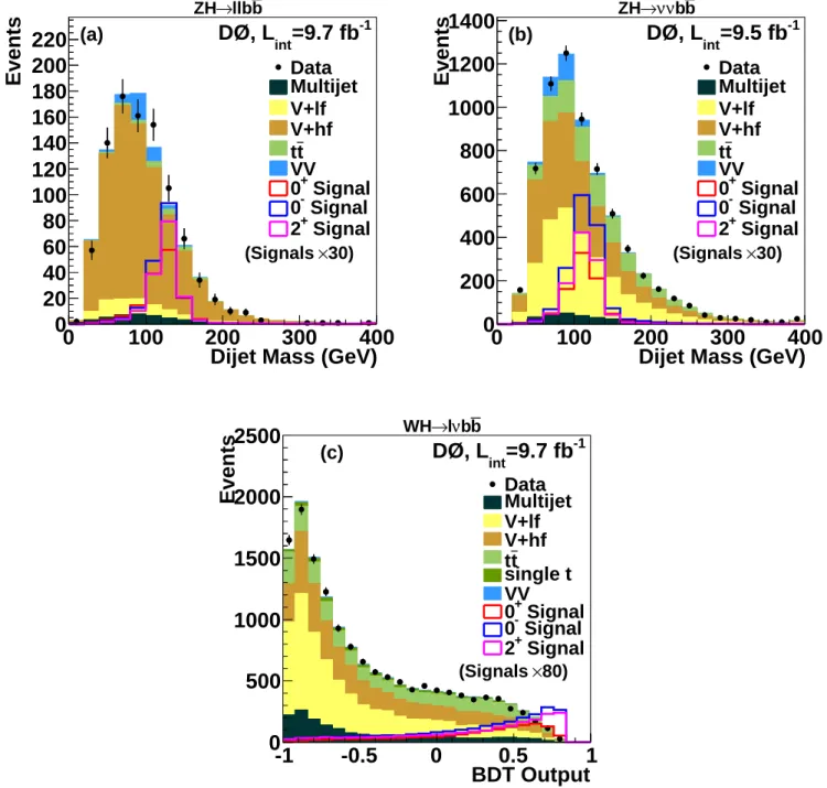
To improve the discrimination between the non-SM signals and backgrounds in the ℓℓb¯b and ννb¯b final states, we use the invariant mass of the dijet system, Mjj, to

select two regions with different signal purities. Events with dijet masses in the range 100 ≤ Mjj ≤ 150 GeV

(70 ≤ Mjj < 150 GeV) for ℓℓb¯b (ννb¯b) final states

com-prise the “high-purity” region (HP), while the remaining events are in the “low-purity region” (LP). As a result of the kinematic fit, the HP region for the ℓℓb¯b final state is narrower than that for the ννb¯b final state, given the correspondingly narrower dijet mass peak. For the ℓνb¯b final state we use the final BDT output (D) of the SM Higgs boson search[19]. Since events with D ≤ 0 provide negligible sensitivity to SM or non-SM signals, we do not consider them further. We separate the remaining events into two categories with different signal purities. The LP

category consists of events with 0 ≤ D ≤ 0.5, and the HP category of events with D > 0.5.

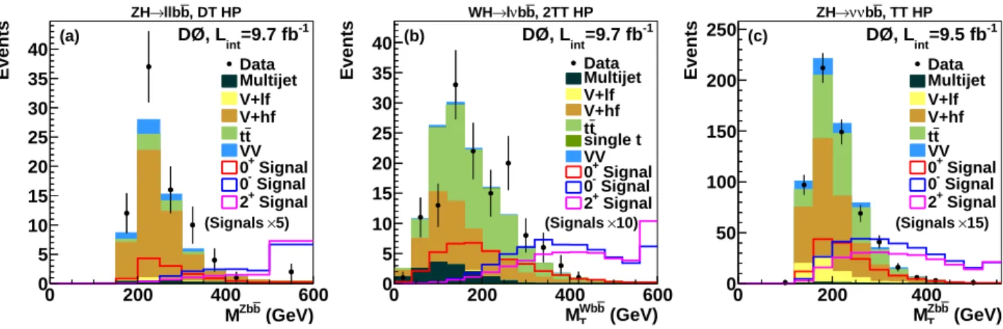
Figure 1 illustrates the discriminating variables for the three analysis channels in the high-purity categories for the most sensitive b-tagging selections. Distributions for additional subchannels can be found in Ref. [40].

We perform the statistical analysis using a modified frequentist approach [38, 41, 42]. We use a negative log-likelihood ratio (LLR) as the test statistic for two hy-potheses: the null hypothesis, H0, and the test

hypothe-sis, H1. This LLR is given by LLR = −2 ln (LH1/LH0), where LHx is the joint likelihood for hypothesis x evalu-ated over the number of bins in the final discriminating variable distribution in each channel. To decrease the effect of systematic uncertainties on the sensitivity, we fit the signals and backgrounds by maximizing the likeli-hood functions by allowing the systematic effects to vary within Gaussian constraints. This fit is performed sepa-rately for both the H0 and H1 hypotheses for the data

and each pseudo-experiment.

We define CLsas CLH1/CLH0where CLHxfor a given hypothesis Hx is CLHx = PHx(LLR ≥ LLR

obs

), and LLRobs_{is the LLR value observed in the data. P}

Hxis de-fined as the probability that the LLR falls beyond LLRobs for the distribution of LLR populated by the Hx model.

For example, if CLs≤ 0.05 we exclude the H1hypothesis

in favor of the H0hypothesis at ≥ 95% CL.

Systematic uncertainties affecting both shape and rate are considered. The systematic uncertainties for each in-dividual analysis are described in Refs. [18–20]. A sum-mary of the major contributions follows. The largest contribution for all analyses is from the uncertainties on the cross sections of the simulated V + heavy-flavor jets backgrounds which are 20%–30%. All other cross section uncertainties for simulated backgrounds are less than 10%. Since the multijet background is estimated from data, its uncertainty depends on the size of the data sample from which it is estimated, and ranges from 10% to 30%. All simulated samples for the W H → ℓνb¯b and ZH → ννb¯b analyses have an uncertainty of 6.1% from the integrated luminosity [43], whereas the simu-lated samples from the ZH → ℓℓb¯b analysis have un-certainties ranging from 0.7%–7% arising from the fit-ted normalization to the data [18]. All analyses take into account uncertainties on the jet energy scale, res-olution, and jet identification efficiency for a combined uncertainty of ≈ 7%. The uncertainty on the b-tagging rate varies from 1%–10% depending on the number and quality of the tagged jets. The correlations between the three analyses are described in Ref. [38].

In this Letter, the H0 hypothesis always contains SM

background processes and the SM Higgs boson normal-ized to µ × σSM

0+ . To test the non-SM cross section we assign the H1 hypothesis as the sum of the JP = 0−

or JP _{= 2}+ _{signal plus SM background processes, with}

(GeV) b Zb M 0 200 400 600 Events 0 5 10 15 20 25 30 35 40 -1 =9.7 fb int DØ, L 5) × (Signals Data Multijet V+lf V+hf t t VV Signal + 0 Signal -0 Signal + 2 , DT HP b llb → ZH (a) (GeV) b Wb T M 0 200 400 600 Events 0 5 10 15 20 25 30 35 40 -1 =9.7 fb int DØ, L 10) × (Signals Data Multijet V+lf V+hf t t single t VV Signal + 0 Signal -0 Signal + 2 , 2TT HP b b ν l → WH (b) (GeV) b Zb T M 0 200 400 Events 0 50 100 150 200 250 -1 =9.5 fb int DØ, L 15) × (Signals Data Multijet V+lf V+hf t t VV Signal + 0 Signal -0 Signal + 2 , TT HP b b ν ν → ZH (c)

FIG. 1: (color online) (a) Invariant mass of the ℓℓb¯b system in the ZH → ℓℓb¯b high-purity double-tag (DT HP) channel, (b) transverse mass of the ℓνb¯b system in the W H → ℓνb¯b high-purity 2-tight-tag (2TT HP) channel, and (c) transverse mass of the ννb¯b system in the ZH → ννb¯b high-purity tight-tag (TT HP) channel. The JP _{= 0}−_{and J}P _{= 2}+

samples are normalized to the product of the SM cross section and branching fraction multiplied by an additional factor. Heavy- and light-flavor quark jets are denoted by lf and hf, respectively. Overflow events are included in the highest mass bin. For all signals, a mass of 125 GeV for the H or X boson is assumed.

the CLs values using signal cross sections expressed as

µ × σSM

0+ and evaluate the expected values for each of these quantities by replacing LLRobs with LLRexp₀+, the median expectation for the JP _{= 0}+ _{hypothesis only.}

Figure 2 illustrates the LLR distributions for the H0 and

JP _{= 2}+_H

1hypotheses, and the observed LLR value

as-suming µ = 1.0, a production rate compatible with both Tevatron and LHC Higgs boson measurements. The sim-ilar plot for JP _{= 0}− _{is shown in Ref. [40]. We interpret}

1 − CLsas the confidence level at which we exclude the

non-SM hypothesis for the models considered in favor of the SM prediction of JP _{= 0}+ _{for the given value of µ.}

For µ = 1.0 we exclude the JP _{= 0}−_(JP _{= 2}+₎

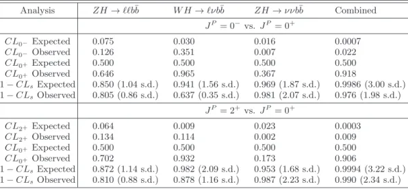
hypothe-sis at the 97.6% (99.0%) CL. The expected exclusions are at the 99.86% and 99.94% CL. Results, including those for µ = 1.23, are given in Table I.

Tables detailing the CLHx values for each individual analysis channel and the combination can be found in Ref. [40]. We also obtain 1 −CLsover a range of SM and

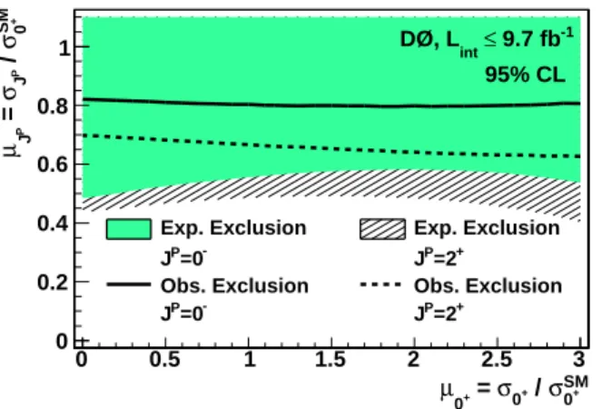
non-SM signal strengths. Figure 3 shows the expected and observed 95% CL exclusions as a function of the JP _{= 0}−_(JP _{= 2}+_{) and J}P _{= 0}+_{signal strengths, which}

may differ between the SM and non-SM signals. In the tests shown in Fig. 3 the signal in the H1hypothesis is the

JP _{= 0}−_(JP _{= 2}+_{) signal normalized to µ}

0−(µ2+)×σSM 0+ , and the signal in the H0hypothesis is the JP = 0+signal

normalized to µ0+× σSM 0+ .

We also consider the possibility of a combination of JP _{signals in our data (e.g., J}P _{= 0}+ _{and J}P _{= 0}−_).

These tests provide constraints on a number of theoreti-cal models such as those containing pseudostheoreti-calar bosons in addition to a SM-like Higgs boson. For these studies we fix the sum of the two cross sections to a specific value of µ×σSM

0+ and vary the fractions f0−= σ0−/(σ0++ σ₀−) or f2+ = σ₂+/(σ₀+ + σ₂+) of non-SM signal and

calcu-LLR -60 -40 -20 0 20 40 60 Pseudoexperiments 0 200 400 600 800 1000 1200 1400 1600 1800 2000 2200 LLR + 0 1 s.d. ± LLR + 0 2 s.d. ± LLR + 0 LLR + 2 Observed LLR -1 9.7 fb ≤ int DØ, L =1.0 µ b Vb → VX

FIG. 2: (color online) LLR distributions comparing the JP ₌

0+

and the JP _{= 2}+

hypotheses for the combination. The JP _{= 0}+

and JP _{= 2}+

samples are normalized to the product of the SM cross section and branching fraction. The vertical solid line represents the observed LLR value assuming µ = 1.0, while the dark and light shaded areas represent the 1 and 2 standard deviations (s.d.) on the expectation from the null hypothesis H0, respectively.

late the same CLs values as above as a function of f0− or f2+. To study f₀−, we now modify H1 to be the sum of the background, the JP _{= 0}− _{signal normalized to}

µ × σSM

0+ × f0−, and the J

P _{= 0}+ _{signal normalized to}

µ × σSM

0+ × (1 − f0−). H0 remains as previously defined. We follow an identical prescription for JP _{= 2}+_{. Figure 4}

presents the value 1 − CLsas a function of the JP = 0−

signal fraction f0− for the case of µ = 1.0, and the corre-sponding figure for the JP _{= 2}+_{hypothesis is available in}

Ref. [40]. For µ = 1.0 we exclude a JP _{= 0}− _(JP _{= 2}+₎

SM + 0 σ / + 0 σ = + 0 µ 0 0.5 1 1.5 2 2.5 3 SM+0 σ / _P J σ = _P J µ 0 0.2 0.4 0.6 0.8 1

Exp. Exclusion Exp. Exclusion

-=0

P

J _JP=2+

Obs. Exclusion Obs. Exclusion

-=0 P J _JP₌₂+ -1 9.7 fb ≤ int DØ, L 95% CL

FIG. 3: (color online) The expected exclusion region (shaded area) and observed exclusion (solid line) as functions of the JP _{= 0}−_{and J}P _{= 0}+

signal strengths. The expected exclu-sion region (hatched area) and observed excluexclu-sion (dashed line) as functions of the JP _{= 2}+

and JP _{= 0}+ signal strengths. Fraction

FIG. 4: (color online) 1 − CLs as a function of the JP =

0− _{signal fraction assuming the product of the total cross}

section and branching ratio is equal to the SM prediction. The horizontal blue line corresponds to the 95% CL exclusion. The dark and light shaded regions represent the 1 and 2 standard deviations (s.d.) fluctuations for the JP _{= 0}+ _hypothesis.

The expected exclusions are f0− > 0.54 (f2+ > 0.47). Limits on admixture fractions for other choices of µ are shown in [40].

In summary, we have performed tests of models with non-SM spin and parity assignments in Higgs boson pro-duction with a W or Z boson and decaying into b¯b pairs. We use the published analyses of the W H → ℓνb¯b, ZH → ℓℓb¯b, and ZH → ννb¯b final states with no mod-ifications to the event selections. Sensitivity to non-SM JP _{assignments in the two models considered here is}

en-hanced via the separation of samples into high- and low-purity categories wherein the total mass or total trans-verse mass of the VX system provides powerful

discrim-ination. Assuming a production rate compatible with both Tevatron and LHC Higgs boson measurements, our data strongly reject non-SM JP _{predictions, and agree}

with the SM JP _{= 0}+ _{prediction. Under the assumption}

of two nearly degenerate bosons with different JP _values,

we set upper limits on the fraction of non-SM signal in our data. This is the first exclusion of non-SM JP

pa-rameter space in a fermionic decay channel of the Higgs boson.

JP

1 − CLs (s.d.) fJP

µ= 1.0 Exp. Obs. Exp. Obs.

0− _{0.9986 (3.00) 0.976 (1.98) >0.54 >0.80} 2+ _{0.9994 (3.22) 0.990 (2.34) >0.47 >0.67} µ= 1.23 0− _{0.9998 (3.60) 0.995 (2.56) >0.45 >0.67} 2+ 0.9999 (3.86) 0.998 (2.91) >0.40 >0.56

TABLE I: Expected and observed 1 − CLs values (converted

to s.d. in parentheses) and signal fractions for µ = 1.0 and µ= 1.23 excluded at the 95% CL.

We thank the staffs at Fermilab and collaborating in-stitutions, and acknowledge support from the DOE and NSF (USA); CEA and CNRS/IN2P3 (France); MON, NRC KI and RFBR (Russia); CNPq, FAPERJ, FAPESP and FUNDUNESP (Brazil); DAE and DST (India); Col-ciencias (Colombia); CONACyT (Mexico); NRF (Ko-rea); FOM (The Netherlands); STFC and the Royal So-ciety (United Kingdom); MSMT and GACR (Czech Re-public); BMBF and DFG (Germany); SFI (Ireland); The Swedish Research Council (Sweden); and CAS and CNSF (China).

[1] G. Aad et al. [ATLAS Collaboration], Phys. Lett. B 716, 1 (2012).

[2] S. Chatrchyan et al. [CMS Collaboration], Phys. Lett. B 716_{, 30 (2012).}

[3] T. Aaltonen et al. [CDF and D0 Collaborations], Phys. Rev. Lett. 109, 071804 (2012).

[4] S. Chatrchyan et al., [CMS Collaboration], Nat. Phys. 10_{, 557 (2014).}

[5] L. Landau, Dokl. Akad. Nauk Ser. Fiz. 60, 207 (1948). [6] C. N. Yang, Phys. Rev. 77, 242 (1950).

[7] T. D. Lee, Phys. Rev. D 8, 1226 (1973).

[8] E. Cerver´o and J.-M. G´erard, Phys. Lett. B 712, 255 (2012).

[9] R. Fok, C. Guimaraes, R. Lewis, and V. Sanz, J. High Energy Phys. 12, 062 (2012).

[10] S. Chatrchyan et al. [CMS Collaboration], Phys. Rev. Lett. 110, 081803 (2013).

[11] G. Aad et al. [ATLAS Collaboration], Phys. Lett. B 726, 120 (2013).

[12] S. Chatrchyan et al. [CMS Collaboration], J. High Energy Phys. 01, 096 (2014).

[13] S. Chatrchyan et al. [CMS Collaboration], Phys. Rev. D 89, 092007 (2014).

[14] S. Chatrchyan et al. [CMS Collaboration], arXiv:1407.0558, (2014), submitted to Eur. Phys. J. C. [15] J. Ellis, D. S. Hwang, V. Sanz, and T. You, J. High

Energy Phys. 12, 134 (2012).

[16] J. Ellis, V. Sanz, and T. You, Eur. Phys. J. C 73 (2013). [17] D. Miller, S. Choi, B. Eberle, M. M¨uhlleitner, and P.

Zer-was, Phys. Lett. B 505, 149 (2001).

[18] V. M. Abazov et al. [D0 Collaboration], Phys. Rev. D 88, 052010 (2013).

[19] V. M. Abazov et al. [D0 Collaboration], Phys. Rev. D 88_{, 052008 (2013).}

[20] V. M. Abazov et al. [D0 Collaboration], Phys. Lett. B 716, 285 (2012).

[21] V. M. Abazov et al. [D0 Collaboration], Nucl. Instrum. Methods Phys. Res. A 565, 463 (2006).

[22] M. Abolins et al., Nucl. Instrum. Methods Phys. Res. A 584_{, 75 (2008).}

[23] R. Angstadt et al., Nucl. Instrum. Methods Phys. Res. A 622, 298 (2010).

[24] M. L. Mangano, M. Moretti, F. Piccinini, R. Pittau, and A. D. Polosa, J. High Energy Phys. 07, 001 (2003). [25] E. E. Boos, V. E. Bunichev, L. V. Dudko, V. I. Savrin,

and V. V. Sherstnev, Phys. Atom. Nucl. 69, 1317 (2006). [26] T. Sj¨ostrand, S. Mrenna, and P. Z. Skands, J. High

En-ergy Phys. 05, 026 (2006).

[27] J. Alwall, M. Herquet, F. Maltoni, O. Mattelaer, and T. Stelzer, J. High Energy Phys. 06, 128 (2011). We use

version 1.4.8.4.

[28] L. Randall and R. Sundrum, Phys. Rev. Lett. 83, 3370 (1999).

[29] L. Randall and R. Sundrum, Phys. Rev. Lett. 83, 4690 (1999).

[30] K. Hagiwara, J. Kanzaki, Q. Li, and K. Mawatari, Eur. Phys. J. C 56, 435 (2008).

[31] P. Aquino, K. Hagiwara, Q. Li, and F. Maltoni, J. High Energy Phys. 11, 1 (2011).

[32] J. Baglio and A. Djouadi, J. High Energy Phys. 10, 064 (2010).

[33] O. Brein, R. V. Harlander, M. Wiesemann, and T. Zirke, Eur. Phys. J. C 72, 1 (2012).

[34] V. M. Abazov et al. [D0 Collaboration], Nucl. In-strum. Methods Phys. Res. A 763, 290 (2014).

[35] V. M. Abazov et al. [D0 Collaboration], Nucl. In-strum. Methods Phys. Res. A 620, 490 (2010).

[36] J. Beringer et al., Particle Data Group, Phys. Rev. D 86, 010001 (2012), and 2013 partial update for the 2014 edition.

[37] A. Hoecker et al., PoS ACAT, 040 (2007). We use version 4.1.0.

[38] V. M. Abazov et al. [D0 Collaboration], Phys. Rev. D 88, 052011 (2013).

[39] T. Aaltonen et al. [CDF and D0 Collaborations], Phys. Rev. D 88, 052014 (2013).

[40] See Supplemental Material.

[41] A. L. Read, J. Phys. G 28, 2693 (2002). [42] W. Fisher, FERMILAB-TM-2386-E (2007). [43] T. Andeen et al., FERMILAB-TM-2365 (2007).

SUPPLEMENTAL MATERIAL

In this document we provide supplemental information on the constraints on models with non-SM spin and parity for the Higgs boson in the V H → V b¯b final states in up to 9.7 fb−1 _{of p¯p collisions at} √_{s = 1.96 TeV collected with}

the D0 detector at the Fermilab Tevatron Collider. We denote a non-SM Higgs boson as X.

Figure 5: Dijet mass distributions for the ννb¯b and ℓℓb¯b analyses and the BDT output distribution for the ℓνb¯b analysis.

Figures 6–9: Additional VX invariant and transverse mass distributions for individual analyses. Figures 10 and 11: LLR distributions for the individual analyses and their combination.

Tables II and III: Tables of CLHx and 1 − CLsvalues for the individual analyses and their combination for µ = 1.0 and µ = 1.23.

Figure 12: _{1 − CLs}as a function of the JP _{= 2}+ _{signal fraction, f}

2+, for all analyses combined.

Figure 13: The expected and observed 95% CL exclusion as functions of the JP _{= 0}− _(JP _{= 2}+_{) signal fraction,}

Dijet Mass (GeV)

0

100

200

300

400

Events

0

20

40

60

80

100

120

140

160

180

200

220

DØ, L

=9.7 fb

30)

×

(Signals

Data

Multijet

V+lf

V+hf

t

t

VV

Signal

0

Signal

-0

Signal

2

(a)

Dijet Mass (GeV)

0

100

200

300

400

Events

0

200

400

600

800

1000

1200

1400

=9.5 fb

DØ, L

30)

×

(Signals

Data

Multijet

V+lf

V+hf

t

t

VV

Signal

0

Signal

-0

Signal

2

(b)

BDT Output

-1

-0.5

0

0.5

1

Events

0

500

1000

1500

2000

2500

=9.7 fb

DØ, L

80)

×

(Signals

Data

Multijet

V+lf

V+hf

t

t

single t

VV

Signal

0

Signal

-0

Signal

2

(c)

FIG. 5: Invariant mass of the dijet system for (a) the ZH → ℓℓb¯b analysis, and (b) the ZH → ννb¯b analysis, and the BDT output for (c) the W H → ℓνb¯b analysis. The JP _{= 2}+ _{and J}P _{= 0}− _{samples are normalized to the product of the SM cross}

section and branching fraction multiplied by an additional factor. Heavy- and light-flavor quark jets are denoted by lf and hf, respectively. Overflow events are included in the highest bin. For all signals, a mass of 125 GeV for the H or X boson is assumed.

(GeV)

M

0

200

400

600

Events

0

20

40

60

80

100

120

=9.7 fb

DØ, L

20)

×

(Signals

Data

Multijet

V+lf

V+hf

t

t

VV

Signal

0

Signal

-0

Signal

2

(a)

(GeV)

M

0

200

400

600

Events

0

5

10

15

20

25

30

35

40

=9.7 fb

DØ, L

5)

×

(Signals

Data

Multijet

V+lf

V+hf

t

t

VV

Signal

0

Signal

-0

Signal

2

(b)

(GeV)

M

0

200

400

600

Events

0

50

100

150

200

250

=9.7 fb

DØ, L

100)

×

(Signals

Data

Multijet

V+lf

V+hf

t

t

VV

Signal

0

Signal

-0

Signal

2

(c)

(GeV)

M

0

200

400

600

Events

0

10

20

30

40

50

60

70

=9.7 fb

DØ, L

30)

×

(Signals

Data

Multijet

V+lf

V+hf

t

t

VV

Signal

0

Signal

-0

Signal

2

(d)

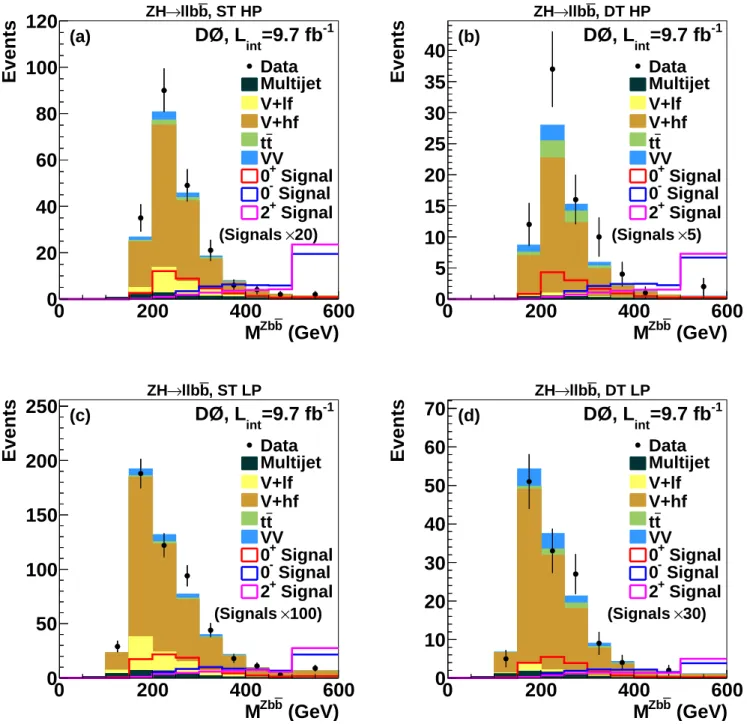
FIG. 6: Invariant mass of the ℓℓb¯b system in the ZH → ℓℓb¯b analysis for events in the (a) single-tag high-purity (ST HP), (b) double-tag high-purity (DT HP), (c) single-tag low-purity (ST LP), and (d) double-tag low-purity (DT LP) channels. The JP _{= 2}+

and JP _{= 0}−_{samples are normalized to the product of the SM cross section and branching fraction multiplied by an}

additional factor. Heavy- and light-flavor quark jets are denoted by lf and hf, respectively. Overflow events are included in the last bin. For all signals, a mass of 125 GeV for the H or X boson is assumed.

(GeV)

M

0

200

400

600

Events

0

50

100

150

200

250

=9.7 fb

DØ, L

30)

×

(Signals

Data

Multijet

V+lf

V+hf

t

t

single t

VV

Signal

0

Signal

-0

Signal

2

(a)

(GeV)

M

0

200

400

600

Events

0

10

20

30

40

50

60

70

80

90

100

=9.7 fb

DØ, L

30)

×

(Signals

Data

Multijet

V+lf

V+hf

t

t

single t

VV

Signal

0

Signal

-0

Signal

2

(b)

(GeV)

M

0

200

400

600

Events

0

10

20

30

40

50

=9.7 fb

DØ, L

10)

×

(Signals

Data

Multijet

V+lf

V+hf

t

t

single t

VV

Signal

0

Signal

-0

Signal

2

(c)

(GeV)

M

0

200

400

600

Events

0

5

10

15

20

25

30

35

40

=9.7 fb

DØ, L

10)

×

(Signals

Data

Multijet

V+lf

V+hf

t

t

single t

VV

Signal

0

Signal

-0

Signal

2

(d)

FIG. 7: Transverse mass of the ℓνb¯b system in the W H → ℓνb¯b analysis in the high-purity (HP) region for (a) 1 tight-tag (1TT), (b) 2 loose-tags (2LT), (c) 2 medium-tags (2MT), and (d) 2 tight-tags (2TT) channels. The JP _{= 2}+

and JP _{= 0}−_samples

are normalized to the product of the SM cross section and branching fraction multiplied by an additional factor. Heavy- and light-flavor quark jets are denoted by lf and hf, respectively. Overflow events are included in the last bin. For all signals, a mass of 125 GeV for the H or X boson is assumed.

(GeV)

M

0

200

400

600

Events

0

100

200

300

400

500

600

700

800

900

1000

=9.7 fb

DØ, L

100)

×

(Signals

Data

Multijet

V+lf

V+hf

t

t

single t

VV

Signal

0

Signal

-0

Signal

2

(a)

(GeV)

M

0

200

400

600

Events

0

20

40

60

80

100

120

140

160

180

200

=9.7 fb

DØ, L

100)

×

(Signals

Data

Multijet

V+lf

V+hf

t

t

single t

VV

Signal

0

Signal

-0

Signal

2

(b)

(GeV)

M

0

200

400

600

Events

0

20

40

60

80

100

120

=9.7 fb

DØ, L

50)

×

(Signals

Data

Multijet

V+lf

V+hf

t

t

single t

VV

Signal

0

Signal

-0

Signal

2

(c)

(GeV)

M

0

200

400

600

Events

0

20

40

60

80

100

120

=9.7 fb

DØ, L

30)

×

(Signals

Data

Multijet

V+lf

V+hf

t

t

single t

VV

Signal

0

Signal

-0

Signal

2

(d)

FIG. 8: Transverse mass of the ℓνb¯b system in the W H → ℓνb¯b analysis in the low purity (LP) region for (a) 1-tight-tag (1TT), (b) 2-loose-tags (2LT), (c) 2-medium-tags (2MT), and (d) 2-tight-tags (2TT) channels. The JP _{= 2}+

and JP _{= 0}−_samples

are normalized to the product of the SM cross section and branching fraction multiplied by an additional factor. Heavy- and light-flavor quark jets are denoted by lf and hf, respectively. Overflow events are included in the last bin. For all signals, a mass of 125 GeV for the H or X boson is assumed.

(GeV)

M

0

200

400

Events

0

200

400

600

800

1000

1200

1400

=9.5 fb

DØ, L

60)

×

(Signals

Data

Multijet

V+lf

V+hf

t

t

VV

Signal

0

Signal

-0

Signal

2

(a)

(GeV)

M

0

200

400

Events

0

50

100

150

200

250

=9.5 fb

DØ, L

15)

×

(Signals

Data

Multijet

V+lf

V+hf

t

t

VV

Signal

0

Signal

-0

Signal

2

(b)

(GeV)

M

0

200

400

Events

0

100

200

300

400

500

600

700

800

DØ, L

=9.5 fb

300)

×

(Signals

Data

Multijet

V+lf

V+hf

t

t

VV

Signal

0

Signal

-0

Signal

2

(c)

(GeV)

M

0

200

400

Events

0

20

40

60

80

100

120

140

160

DØ, L

=9.5 fb

150)

×

(Signals

Data

Multijet

V+lf

V+hf

t

t

VV

Signal

0

Signal

-0

Signal

2

(d)

FIG. 9: Transverse mass of the ννb¯b system in the ZH → ννb¯b analysis for events in the (a) medium-tag high-purity (MT HP), (b) tight-tag high-purity (TT HP), (c) medium-tag low-purity (MT LP), and (d) tight-tag low-purity (TT LP) channels. The JP _{= 2}+

and JP _{= 0}− _{samples are normalized to the product of the SM cross section and branching fraction multiplied}

by an additional factor. Heavy- and light-flavor quark jets are denoted by lf and hf, respectively. Overflow events are included in the last bin. For all signals, a mass of 125 GeV for the H or X boson is assumed.

LLR -20 -10 0 10 20 Pseudoexperiments 0 500 1000 1500 2000 2500 3000 0+ LLR 1 s.d. ± LLR + 0 2 s.d. ± LLR + 0 LLR

FIG. 10: LLR distributions comparing the JP _{= 0}+

and the JP _{= 0}− _{hypotheses for the (a) ZH → ℓℓb¯b analysis, (b)}

W H → ℓνb¯b analysis, (c) ZH → ννb¯b analysis, and (d) their combination. The JP _{= 0}+

and JP _{= 0}−_{samples are normalized}

to the product of the SM cross section and branching fraction multiplied by µ = 1.0. The vertical solid line represents the observed LLR value, while the dark and light shaded areas represent 1 s.d. and 2 s.d. on the expectation from the null hypothesis H0, respectively. Here H0is the SM JP = 0+signal plus backgrounds. For all signals, a mass of 125 GeV for the H or X boson

LLR -20 -10 0 10 20 Pseudoexperiments 0 500 1000 1500 2000 2500 3000 3500 4000 4500 ₀+ _LLR 1 s.d. ± LLR + 0 2 s.d. ± LLR + 0 LLR + 2 Observed LLR -1 = 9.7 fb int DØ, L =1.0 µ b llb → VX (a) LLR -40 -20 0 20 40 Pseudoexperiments 0 200 400 600 800 1000 1200 1400 1600 1800 2000 2200 LLR + 0 1 s.d. ± LLR + 0 2 s.d. ± LLR + 0 LLR + 2 Observed LLR -1 = 9.7 fb int DØ, L =1.0 µ b b ν l → VX (b) LLR -40 -20 0 20 40 Pseudoexperiments 0 200 400 600 800 1000 1200 1400 1600 1800 2000 2200 ₀+ _LLR 1 s.d. ± LLR + 0 2 s.d. ± LLR + 0 LLR + 2 Observed LLR -1 = 9.5 fb int DØ, L =1.0 µ b b ν ν → VX (c) LLR -60 -40 -20 0 20 40 60 Pseudoexperiments 0 200 400 600 800 1000 1200 1400 1600 1800 2000 2200 LLR + 0 1 s.d. ± LLR + 0 2 s.d. ± LLR + 0 LLR + 2 Observed LLR -1 9.7 fb ≤ int DØ, L =1.0 µ b Vb → VX (d)

FIG. 11: LLR distributions comparing the JP _{= 0}+

and the JP _{= 2}+

hypotheses for the (a) ZH → ℓℓb¯b analysis, (b) W H → ℓνb¯b analysis, (c) ZH → ννb¯b analysis, and (d) their combination. The JP _{= 0}+

and JP _{= 2}+

samples are normalized to the product of the SM cross section and branching fraction multiplied by µ = 1.0. The vertical solid line represents the observed LLR value, while the dark and light shaded areas represent 1 s.d. and 2 s.d. on the expectation from the null hypothesis H0, respectively. Here H0is the SM JP = 0+signal plus backgrounds. For all signals, a mass of 125 GeV for the H or X boson

Analysis _{ZH → ℓℓb¯b W H → ℓνb¯b ZH → ννb¯b} Combined JP _{= 0}− _{vs. J}P _{= 0}+ CL0− Expected 0.075 0.030 0.016 0.0007 CL0− Observed 0.126 0.351 0.007 0.022 CL0+ Expected 0.500 0.500 0.500 0.500 CL0+ Observed 0.646 0.965 0.367 0.918 1 − CLs Expected 0.850 (1.04 s.d.) 0.941 (1.56 s.d.) 0.969 (1.87 s.d.) 0.9986 (3.00 s.d.) 1 − CLs Observed 0.805 (0.86 s.d.) 0.637 (0.35 s.d.) 0.981 (2.07 s.d.) 0.976 (1.98 s.d.) JP _{= 2}+ _{vs. J}P _{= 0}+ CL2+ Expected 0.064 0.009 0.023 0.0003 CL2+ Observed 0.134 0.114 0.002 0.009 CL0+ Expected 0.500 0.500 0.500 0.500 CL0+ Observed 0.702 0.932 0.173 0.906 1 − CLs Expected 0.872 (1.14 s.d.) 0.982 (2.09 s.d.) 0.953 (1.68 s.d.) 0.9994 (3.22 s.d.) 1 − CLs Observed 0.810 (0.88 s.d.) 0.878 (1.16 s.d.) 0.987 (2.23 s.d.) 0.990 (2.34 s.d.)

TABLE II: Expected and observed CLHx and 1 − CLs values for J

P _{= 0}−_{and J}P _{= 2}+

VX associated production, assuming signal cross sections equal to the 125 GeV SM Higgs production cross section multiplied by µ = 1.0. The null hypothesis is taken to be the sum of the SM Higgs boson signal and background production.

Analysis _{ZH → ℓℓb¯b W H → ℓνb¯b ZH → ννb¯b} Combined JP _{= 0}− _{vs. J}P _{= 0}+ CL0− Expected 0.046 0.012 0.005 <0.0001 CL0− Observed 0.072 0.245 0.0006 0.005 CL0+ Expected 0.500 0.500 0.500 0.500 CL0+ Observed 0.615 0.971 0.215 0.922 1 − CLs Expected 0.908 (1.33 s.d.) 0.975 (1.96 s.d.) 0.989 (2.31 s.d.) 0.9998 (3.60 s.d.) 1 − CLs Observed 0.883 (1.19 s.d.) 0.747 (0.67 s.d.) 0.997 (2.78 s.d.) 0.995 (2.56 s.d.) JP _{= 2}+ _{vs. J}P _{= 0}+ CL2+ Expected 0.037 0.003 0.009 <0.0001 CL2+ Observed 0.078 0.056 0.003 0.002 CL0+ Expected 0.500 0.500 0.500 0.500 CL0+ Observed 0.679 0.937 0.363 0.911 1 − CLs Expected 0.925 (1.44 s.d.) 0.995 (2.56 s.d.) 0.983 (2.11 s.d.) 0.9999 (3.86 s.d.) 1 − CLs Observed 0.885 (1.20 s.d.) 0.941 (1.56 s.d.) 0.991 (2.35 s.d.) 0.998 (2.91 s.d.)

TABLE III: Expected and observed CLHx and 1 − CLsvalues for J

P _{= 0}−_{and J}P _{= 2}+

VX associated production, assuming signal cross sections equal to the 125 GeV SM Higgs production cross section multiplied by µ = 1.23. The null hypothesis is taken to be the sum of the SM Higgs boson signal and background production.

Fraction

+

2

0.1

0.2

0.3

0.4

0.5

0.6

0.7

0.8

0.9

1

1-CL

0.7

0.8

0.9

1

1.1

1.2

1.3

9.7 fb

≤

DØ, L

σ

=

σ

+

σ

Observed

1-CL

Expected

1-CL

1 s.d.

±

Expected

2 s.d.

±

Expected

FIG. 12: (color online) 1 − CLs as a function of the JP = 2+ signal fraction f2+ for µ = 1.0 for all analyses combined. The horizontal solid line corresponds to the 95% CL exclusion. The dark and light shaded regions represent the expected 1 and 2 s.d. fluctuations of the JP _{= 0}+