HAL Id: ird-02063040
https://hal.ird.fr/ird-02063040
Submitted on 10 Mar 2019
HAL is a multi-disciplinary open access archive for the deposit and dissemination of sci-entific research documents, whether they are pub-lished or not. The documents may come from teaching and research institutions in France or abroad, or from public or private research centers.
L’archive ouverte pluridisciplinaire HAL, est destinée au dépôt et à la diffusion de documents scientifiques de niveau recherche, publiés ou non, émanant des établissements d’enseignement et de recherche français ou étrangers, des laboratoires publics ou privés.
Analysis of diversification : combining phylogenetic and
taxonomic data
Emmanuel Paradis
To cite this version:
Emmanuel Paradis. Analysis of diversification : combining phylogenetic and taxonomic data. Proceed-ings of the Royal Society B: Biological Sciences, Royal Society, The, 2003, 270 (1532), pp.2499-2505. �10.1098/rspb.2003.2513�. �ird-02063040�
Analysis of diversification: combining
phylogenetic and taxonomic data
Emmanuel Paradis
Laboratoire de Pal´
eontologie, Pal´
eobiologie & Phylog´
enie,
Institut des Sciences de l’ ´
Evolution,
Universit´
e Montpellier II,
F-34095 Montpellier c´
edex 05, France
E-mail: [email protected]
Abstract: The estimation of diversification rates using phylogenetic data has attracted a lot of attention in the last decade. In this context, the analysis of incomplete phylogenies (e.g., phylogenies resolved at the family-level but unresolved at the species-level) has remained difficult. I present here a
likelihood-based method to combine partially resolved phylogenies with taxonomic (species-richness) data in order to estimate speciation and extinction rates. This method is based on fitting a birth-and-death model to both phylogenetic and taxonomic data. Some examples of the method are presented with data on birds and on mammals. The method is compared with existing approaches that deal with incomplete phylogenies. Some perspectives and generalizations of the approach introduced in this paper are further discussed.
Keywords: diversity; estimation; extinction; maximum likelihood; phylogeny; speciation.
1. INTRODUCTION
Evolutionary biology deals with changes in species diversity through time and their mechanisms. Such changes are brought about by speciation and extinction events, and quantifying the rates of these events contributes to a better
understanding of the biological mechanisms of evolution. During the past decade, there has been a lot of interest in using phylogenetic data to estimate speciation and extinction rates. This follows from the increasing number of phylogenetic studies using molecular techniques which has led to resolve the relationships among more and more taxa. Most of the methods to study diversification with phylogenetic data consider phylogenies at the species level, and thus require that most (if not all) species of the studied lineages be included in the reconstructed phylogenies (Hey 1992; Nee et al. 1994a; Sanderson & Donoghue 1996; Paradis 1997, 1998a; Pybus & Harvey 2000). However, quite often phylogenetic data are available at a higher level than the species, for instance giving the relationships among families whereas the relationships among species within the families are unknown though the numbers of species in these groups are known. Examples of such situation are provided by the phylogeny of birds where almost all 144 families are included but about 1000 species out of 9646 are represented (Sibley & Ahlquist 1990), or the phylogeny of Insects where the relationships among the 30 orders have been inferred but the relationships among the more than a million species cannot be drawn (Mayhew 2002).
In this paper, I present a method to estimate speciation and extinction rates which combines phylogenetic and species richness data. Some examples using birds and mammals are presented.
2. METHODS
The approach used here is an extension of the birth–death model developed by Nee et al. (1994a). They used a birth–death process to model phylogenetic diversification and estimate speciation and extinction rates with the branching times from an observed phylogenetic tree. Basically, this method requires that all species belonging to the studied clade are included in the reconstructed tree (Nee et al. 1994a,b).
The present approach assumes that two kinds of information are available. First, the phylogenetic relationships (tree topology and branch lengths) of a subset of all species belonging to the studied clade are known; this is referred to as the phylogenetic data in this paper. It is further assumed that the reconstructed phylogenetic tree is ultrametric, that is the branch lengths are linearly related to time. Second, the number of species belonging to each tip of this reconstructed phylogeny is known as well, and this is called the taxonomic data. This is likely to be a very common situation. For instance, it is usual in a phylogenetic study to resolve the relationships among higher level taxa (e.g., among orders within a class, or among families within an order) and that the number of species in each of these taxa is known. It is assumed below that both the phylogenetic and the taxonomic data are known without error.
Denote N the number of tips in the reconstructed phylogeny, and ni the
number of species belonging to the ith tip (i = 1, . . . N ).
Let us assume that a living species has an instantaneous probability of splitting in two species called the rate of speciation and denoted λ, and an instantaneous probability of disappearing called the rate of extinction and denoted µ. We further assume that both rates are constant through time and across lineages. Under this “birth-and-death” model, we can formulate the probabilities of the observed data
using formulae in Kendall (1948) and in Nee et al. (1994a).
The phylogenetic data are comprised by a set of N lineages that originated from the nodes of the reconstructed phylogeny and survived until present. The probability for a lineage originated at time t of not going extinct at time T is (Nee et al. 1994a, eq. 2):
P (t, T ) = λ − µ
λ − µe−(λ−µ)(T −t). (1)
The probability density of the branching events in the observed tree is
proportional to the number of extant lineages multiplied by λ. It is thus possible to compute the likelihood of the phylogenetic data by multiplying together the probabilities of the observed branching events and the probabilities that the lineages survived until present. This likelihood is:
LP = (N − 1)!λN −2 N
Y
i=3
P2(ti, T )P2(t2, T ). (2)
This is actually a modified likelihood from Nee et al. (1994a, their eq. 20) to take into account the fact that the lineages survived with one or more species untill present.
Let us rewrite equation 1 as:
P (t, T ) = 1 − a
1 − ae−rx, (3)
where a = µ/λ, r = λ − µ, and x = T − t. If T is the present, x is in fact the branching time. Some algebra lead us to rewrite equation 2 as:
LP = (N − 1)!rN −2(1 − a)Nexp 2r N X i=2 xi ! N Y i=2 (erxi − a)−2. (4)
A logarithmic transformation of the above equation leads to an expression easier to manipulate: ln LP = ln(N − 1)! + (N − 2) ln r + N ln(1 − a) + 2r N X i=2 xi− 2 N X i=2 ln(erxi − a). (5)
The taxonomic data are represented by a set of monophyletic groups of species which numbers and dates of origin (the lengths of the terminal branches of the reconstructed tree) are both known. The probability for a lineage originated from a single species to have n species after a time t is (Kendall 1948, eq. 16):
µ(e(λ−µ)t− 1) λ(e(λ−µ)t− µ) if nt= 0, (6) " 1 − µ(e (λ−µ)t− 1) λ(e(λ−µ)t− µ) # (1 − ζt)ζtn−1 if nt > 0, (7) where ζt = λ(e(λ−µ)t− 1) λe(λ−µ)t − µ . (8)
The same reparametrization used above for the phylogenetic data (a = µ/λ, r = λ − µ) and an algebraic development lead us to rewrite equation 7 as:
P (nt = n) =
(1 − a)2ert
(ert− a)n+1(e
rt− 1)n−1 for n ≥ 1. (9)
Multiplying together the corresponding probabilities for the N observed lineages gives the likelihood of the taxonomic data:
LT = (1 − a)2N N
Y
i=1
erti(erti− 1)ni−1(erti− a)−(ni+1), (10)
and after logarithmic transformation:
ln LT = 2N ln(1 − a) + r N X i=1 ti+ N X i=1 (ni− 1) ln(erti− 1) − N X i=1 (ni+ 1) ln(erti− a). (11)
The log-likelihood of the combined phylogenetic and taxonomic data (denoted ln L) is the sum ln LP + ln LT. Given some data, finding the maximum of ln L over
a and r gives their respective maximum likelihood estimates (MLEs) denoted ˆa and ˆr. Under the assumption that ln L is approximately normally distributed around its maximum, it is possible to estimate the standard-errors of the MLEs using its second derivatives.
Practically, maximizing ln L would require us to find its first partial derivatives with respect to a and r; however these expression are too complex to be solved analytically. I used instead a numerical minimization method. The likelihood was transformed as the deviance (equal to −2 ln L); finding the maximum likelihood was equivalent to minimizing the deviance. This was done with the nonlinear minimization function of R (Ihaka & Gentleman 1996) which uses a Newton-type algorithm for unconstrained minimization (Schnabel et al. 1985). This method allows one to find the minimum of a function even when its partial and second derivatives are unknown. However, these derivatives can be computed numerically, allowing to calculate the standard-errors of the MLEs.
If the normal approximation of the likelihood surface is not satisfied (e.g., due to asymmetries), the standard-errors of the MLEs based on the second derivatives of the log-likelihood may be incorrect. An alternative approach is to use the profile
likelihood (Hudson 1971): this consists of looking at the likelihood surface around its maximum. Since a difference between two log-likelihoods less than or equal to 1.92 is not significantly different with P > 0.05 (Edwards 1992), all likelihood values greater than or equal to the maximum likelihood minus 1.92 define a 95 % confidence region for both parameters a and r. This is best visualized by plotting the likelihood surface for different values of the two parameters. The confidence intervals of a and r can then be transformed in confidence intervals of λ and µ by developing the inequalities defining these intervals (see APPENDIX 1).
The programs implementing the method developed here are freely distributed in the package APE (analysis of phylogenetics and evolution, Paradis et al. 2003).
3. EXAMPLES
3.1 Birds
The extensive study of Sibley & Ahlquist (1990) provided an estimate of the phylogenetic relationships for more than 1000 species among the 9646 living bird species based on DNA/DNA hybridization experiments (their famous “tapestry”). This covered all avian orders, and almost all families. Sibley & Monroe (1990) made a review of the taxonomy of birds, and listed the number of species for all taxonomic levels, thus providing the numbers of species for the 23 orders and 144 families of living birds.
The goal of the present analysis was to estimate diversification rates for birds at the order and family levels. The data for 137 families were considered. The seven families not included here were groups with uncertain relationships (Sibley & Ahlquist 1990) and contained very few species: Brachypteraciidae (5 species), Raphidae (3), Mesitornithidae (3), Philepittidae (4), Callaeatidae (3),
dichotomous and contained one trichotomy (see Sibley & Ahlquist 1990, Fig. 356). This was resolved by assuming a null branch length below this node, so that the corresponding branching time was counted twice in the analysis. The original units of Sibley & Ahlquist (∆T50H, a measure of the distance among the tips of the
tree) were used here for the branch lengths.
Twenty three orders were considered: the resulting phylogeny was fully dichotomous (Fig. 1). As for families, the number of species were from Sibley & Monroe 1990.
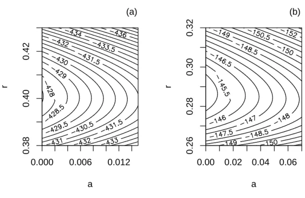
The parameter estimates for the bird family data were ˆa = 0, and ˆr = 0.401 (s.e. = 0.006). The maximum log-likelihood was −427.45. A plot of the
log-likelihood around its maximum shows a 95 % confidence interval of [0, 0.008] for a, and [0.385, 0.418] for r (Fig. 2a). The 95 % confidence intervals for
speciation and extinction rates (in ∆T50H time units) were 0.385 ≤ λ ≤ 0.421, and
0 ≤ µ ≤ 0.003.
The same estimates for the analysis at the order-level were ˆa = 0, and ˆ
r = 0.287 (s.e. = 0.007); the maximum log-likelihood was −144.58. The
log-likelihood surface indicates a 95 % confidence interval of [0, 0.040] for a, and [0.268, 0.308] for r (Fig. 2b). The 95 % confidence intervals for speciation and extinction rates (in ∆T50H time units) were 0.268 ≤ λ ≤ 0.321, and 0 ≤ µ ≤ 0.013.
It is noteworthy that the confidence intervals for λ estimated from family and order data do not overlap. This is discussed below.
3.2 Eutherian Mammals
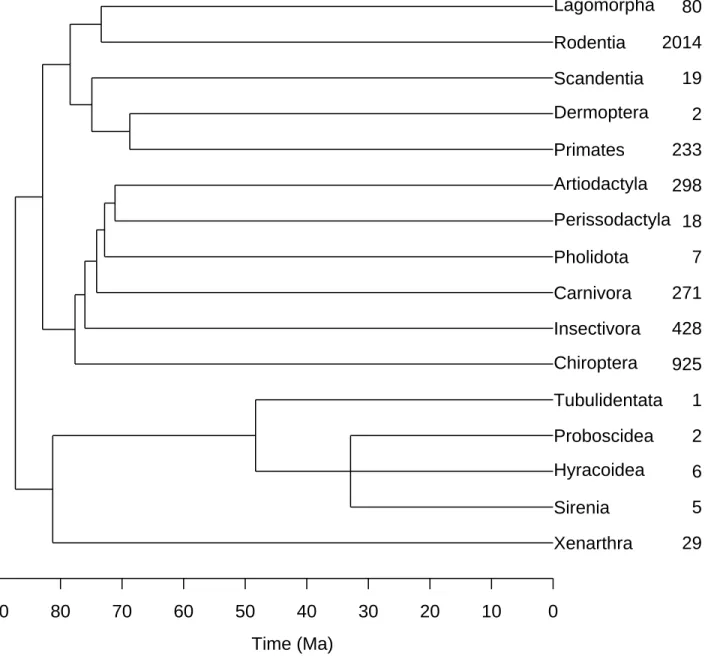
Wilson & Reeder (1993) listed 26 orders of mammals together with a complete taxonomic listing at the species level. On the other hand, there is, for the moment, no complete phylogeny with branch lengths of the orders of mammals. Douzery et
al. (in press) reconstructed a phylogeny with dated nodes for 18 orders of mammals based on molecular data for 42 species. They used a nonparametric method which does not assume a molecular clock (Sanderson 1997) to estimate the divergence dates of the tree. I discarded the data for the order Diprotodontia (represented by the kangaroo Macropus) which was the only non-Eutherian order in this study. I used data for 17 orders among which the species richness of Cetacea (78 species) was pooled with that of Artiodactyla (220 species), thus leaving 16 orders. I considered only Eutherian mammals since the divergence between this clade and the other mammals is not yet well dated (Douzery pers. comm.).
The tree was not fully dichotomous and contained one trichotomy (Fig. 3). This was resolved in the same way than for the phylogeny of avian families. The unit of branch lengths was in million years ago (Ma) calculated from the ages of the nodes reported by Douzery et al. (in press).
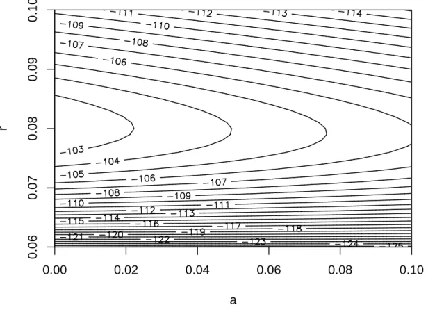
The parameter estimates for this mammalian phylogeny were ˆa = 0, and ˆ
r = 0.080 (s.e. = 0.003). The maximum log-likelihood was −102.21. A plot of the log-likelihood around its maximum shows a 95 % confidence interval of [0, 0.050] for a, and [0.074, 0.088] for r (Fig. 4). The 95 % confidence intervals for speciation and extinction rates are 0.074 ≤ λ ≤ 0.093, and 0 ≤ µ ≤ 0.005.
4. DISCUSSION
There is great interest in using phylogenetic data to study macroevolutionary processes as shown by recent reviews (Sanderson & Donoghue 1996; Barraclough & Nee 2001). Significant progress has been accomplished when the available
phylogeny is complete (i.e., has been reconstructed with all species; Slowinski & Guyer 1993; Harvey et al. 1994). However, the development of approaches for analyzing incomplete phylogenies has been more difficult (Paradis 1997, 1998b;
Pybus & Harvey 2000). The method presented in this paper is an attempt to combine phylogenetic and taxonomic data to estimate speciation and extinction rates, and thus can be used to analyse incomplete phylogenies provided some data on species richness are available.
The present method can be viewed as an extension of the method introduced by Nee et al. (1994a). Both methods are based on the birth-and-death process studied by Kendall (1948). The main distinction between both methods, particularly apparent in the computation of their respective likelihoods, is that Nee et al. (1994a) consider that all surviving lineages have one species living at present, whereas the present method simply assumes that these lineages survive (with one or more species).
It is interesting to point out that both approaches aim to estimate parameters rather than to test hypotheses. Nee et al.’s (1994a) method can be extended to more general birth–death models (e.g., assuming time-dependence in both
parameters, see Nee et al. 1994a) but, as far as I know, this does not seem to have been used in practice. Whether the approach presented here could be extended to more complex birth–death models requires more work. It would be interesting in the future to compare extensively the estimates from Nee et al.’s (1994a) method and the present one.
In a previous work, I developed a method to take into account missing species in phylogenetic data when estimating diversification rates (Paradis 1997, 1998b). This is based on making an analogy between branching times in a phylogeny and survival events: thus missing branching times can be treated as censored data (i.e. when death is not known precisely but it is known that it occurred after some time). This approach has the advantage of making available likelihood-based fitting of alternative models, and thus testing alternative hypotheses on variation
in diversification rates (Paradis 1997, 1998b). However, this has the inconvenient property that when the proportion of missing data is too large there is not enough information to allow efficient estimation. Thus, the approach based on survival models is not applicable to the analysis of the kind of data analysed in the above examples.
Though the approach presented here aims to analyse incomplete phylogenies, the data considered (branch lengths, tree topology, and number of species) are assumed to be known without error. This assumption is likely to be untrue in some situations since the tree is usually an estimate and species numbers in some groups may be inacurrate particularly in speciose or poorly-known groups. The maximum likelihood approach developed here could be, at least in theory,
extended to take into account such uncertainties but this would certainly require complex mathematical developments. Furthermore, it is likely that in most situations the uncertainty in the data reflects conflicts between a limited number of scenarios (such as the attribuation of a sub-group to a particular sub-clade) and thus it is possible to consider alternatively all of them.
Pybus & Harvey (2000) proposed a method to assess the impact of
incompleteness in phylogenetic data on testing for constant diversification. This is based on simulating phylogenies with constant rates then sampling randomly a subset of the species “living” at the end of the simulation. This Monte Carlo approach makes it possible to estimate the distribution of their test statistic (the γ-statistic) in the presence of missing data.
Nee et al. (1994b) used simulations to assess the effect of missing data on analysis of diversification with a graphical method: the lineages-through-time plot (Harvey et al. 1994; Nee et al. 1995). They showed that the analysis of incomplete phylogenies may indicate a spurious decline through time of diversification (Nee et
al. 1994b). There is still an obvious need for methods that would tease apart the effects of incomplete sampling from those of temporal variation in phylogenetic diversification rates.
The analyses presented in this paper have mainly an illustrative purpose, but the results obviously call for a few comments. We will first convert the rates estimated for birds in meaningful units (Ma−1). The depth of the bird tree of Sibley & Ahlquist (1990) is 28 in ∆T50H units. Paton et al. (2002), using various
methods, dated the origin of the modern bird orders between 110 and 130 Ma depending on the method. We need thus, roughly, to multiply Sibley & Ahlquist’s (1990) time-scale by 4 to obtain a time-scale in Ma. Therefore, the corresponding rates converted in Ma−1 (after dividing the above speciation and extinction rates by 4) are 0.096 ≤ λ ≤ 0.105, and 0 ≤ µ ≤ 0.001 for the family-based analysis, and 0.067 ≤ λ ≤ 0.080, and 0 ≤ µ ≤ 0.003 for the order-based one.
Concerning birds, the analysis at the level of orders yielded smaller estimates and larger confidence intervals than the same analysis at the level of families. There could be two explanations for this discrepancy. First, the family-based data can be thought as more accurate than the order-based ones. Consequently, the analysis of the former may give more accurate (with narrower confidence intervals) estimates than for the latter. Second, heterogeneity in rates may affect the present estimates. The present method assumes that speciation and extinction rates are constant through time and the same for all lineages. This is certainly not true for the present data since species richness is extremely uneven among bird families, with some Passerines being extremely diverse (e.g., Fringillidae). It could be that at the level of orders, the effect of heterogeneity was lessened since the
heterogeneity among orders may be smaller than among families. In other words, the family-based estimates may have been “pushed-up” by the many diversified
families of Passerines.
The estimates for mammals are close to those for birds, particularly for the order-based analysis of the latter group. This is in agreement with the slightly younger origin of the modern orders of Eutherian mammals (ca. 90 Ma) compared to birds (ca. 110 Ma). The Eutherian mammals have 4260 species (Mammals total 4628 species according to Wilson & Reeder 1993) against 9623 for the birds
analysed here. However, we need to keep in mind that rates are certainly heterogeneous in both groups: rodents, like passerines for birds, have surely
diversified at a higher rate than other lineages of mammals (see Purvis et al. 1995 and Paradis 1998b for analyses of heterogeneity in diversification rates among lineages of primates; and Mooers & Heard 1997 for a review). However, the present analyses suggest that, on average, birds and mammals have diversified at similar rates.
The three analyses reported in this paper yielded an estimate of a equal to zero. It is obvious that some extinction events occurred during the history of mammals and birds as evidenced by the fossil record. However, the estimation of extinction rates with phylogenies without fossils is still an open issue. For
instance, Purvis et al. (1995) reported estimates of a equal to zero in primate lineages in two cases out of four, and Nee et al. (1994b) reported similar instances in other groups. The method presented in this paper can, in theory, yields
estimates of a greater than zero (APPENDIX 2). One referee of the present paper pointed out that there is currently some confusion in the literature with respect to the issue of estimating extinction rates with phylogenies without fossils (e.g., Sims & McConway 2003). In the absence of an extensive theoretical treatment of this issue, it seems sound to take the estimates of extinction rates inferred from
would be to assess whether the confidence interval for the extinction rate inferred with the profile likelihood correctly covers the true value of µ.
The method presented in this paper has surely a wide range of potential applications. Future research will need to address the issues of temporal variation and heterogeneity in rates. Ultimately, linking the methods dealing with
phylogenetic diversification and the methods dealing with the evolution of characters, such as the various phylogenetic comparative methods, should be a significant progress in evolutionary analysis.
I am grateful to three anonymous referees for their constructive comments on an earlier version of this paper, and to E. Douzery for sending me his results on divergence dates on mammals. This research was financially supported by the Institut Fran¸cais de la Biodiversit´e and the Centre National de la Recherche Scientifique. This is publication 2003-052 of the Institut des Sciences de l’ ´Evolution (Unit´e Mixte de Recherche 5554 du Centre National de la Recherche Scientifique).
APPENDIX 1
This appendix shows how the confidence intervals of the parameters a and r are transformed to give confidence intervals of the speciation and extinction rates (λ and µ, respectively).
Suppose the profile likelihood of the model gives the two 95 % confidence intervals:
a1 ≤ a ≤ a2, (12)
Since we have a = µ/λ, and r = λ − µ, and under the condition that λ is positive nonnull, we can re-write both inequalities as:
a1λ ≤ µ ≤ a2λ, (14)
r1+ µ ≤ λ ≤ r2+ µ. (15)
Thus we have for λ the inequalities:
r1+ a1λ ≤ λ ≤ r2+ a2λ, (16)
which can be written separately as:
r1+ a1λ − λ ≤ 0, 0 ≤ r2+ a2λ − λ. (17)
Developing algebraically both inequalities gives (under the condition that both a1 and a2 are less than one):
r1
1 − a1
≤ λ, r2 1 − a2
≥ λ, (18)
giving the 95 % confidence interval for λ:
r1
1 − a1
≤ λ ≤ r2 1 − a2
. (19)
Substituting in the above inequalities of µ gives its 95 % confidence interval:
a1r1
1 − a1
≤ µ ≤ a2r2 1 − a2
APPENDIX 2
This appendix shows that the method presented in this paper can yield estimates of a greater than zero. This can be shown by examining the first partial derivative of the log-likelihood function ln L. Since ln L = ln LP + ln LT, we have:
∂ ln L ∂a = ∂ ln LP ∂a + ∂ ln LT ∂a . (21)
Deriving equations 5 and 11 with respect to a is straightforward:
∂ ln LP ∂a = 2 N X i=2 1 erxi − a − N 1 − a; (22) ∂ ln LT ∂a = N X i=1 ni+ 1 erti− a − 2N 1 − a; (23)
giving for the log-likelihood function:
∂ ln L ∂a = 2 N X i=2 1 erxi − a + N X i=1 ni+ 1 erti− a − 3N 1 − a. (24)
If the partial derivative of ln L can be positive at a = 0, then ln L can have a maximum for positive values of a. Fixing a = 0 in the above equation gives:
2 N X i=2 1 erxi + N X i=1 ni+ 1 erti − 3N. (25)
The first two terms above are always positive, whereas the third one is always negative. Thus, the above expression can be positive depending on the values of r, xi, ti, and N . Consequently, the log-likelihood can potentially achieve a maximum
REFERENCES
Barraclough, T. G. & Nee, S. 2001 Phylogenetics and speciation. Trends Ecol. Evol. 16, 391–399.
Douzery, E. J. P., Delsuc, F., Stanhope, M. J. & Duchon, H. in press Local molecular clocks in three nuclear genes: divergence times for rodents and other mammals, and incompatibility among fossil calibrations. J. Mol. Evol..
Edwards, A. W. F. 1992 Likelihood (expanded edition). Baltimore: Johns Hopkins University Press.
Harvey, P. H., May, R. M. & Nee, S. 1994 Phylogenies without fossils. Evolution 48, 523–529.
Hey, J. 1992 Using phylogenetic trees to study speciation and extinction. Evolution 46, 627–640.
Hudson, D. J. 1971 Interval estimation from the likelihood function. J. R. Statist. Soc. B 33, 256–262.
Ihaka, R. & Gentleman, R. 1996 R: a language for data analysis and graphics. J. Comput. Graph. Statist. 5, 299–314.
Kendall, D. G. 1948 On the generalized “birth-and-death” process. Ann. Math. Stat. 19, 1–15.
Mayhew, P. J. 2002 Shifts in hexapod diversification and what Haldane could have said. Proc. R. Soc. Lond. B 269, 969–974.
Mooers, A. Ø. & Heard, S. B. 1997 Evolutionary process from phylogenetic tree shape. Quart. Rev. Biol. 72, 31–54.
Nee, S., May, R. M. & Harvey, P. H. 1994a The reconstructed evolutionary process. Phil. Trans. R. Soc. Lond. B 344, 305–311.
Nee, S., Holmes, E. C., May, R. M. & Harvey, P. H. 1994b Extinction rates can be estimated from molecular phylogenies. Phil. Trans. R. Soc. Lond. B 344, 77–82.
Nee, S., Holmes, E. C., Rambaut, A. & Harvey, P. H. 1995 Inferring population history from molecular phylogenies. Phil. Trans. R. Soc. Lond. B 349, 25–31.
Paradis, E. 1997 Assessing temporal variations in diversification rates from
phylogenies: estimation and hypothesis testing. Proc. R. Soc. Lond. B 264, 1141–1147.
Paradis, E. 1998a Testing for constant diversification rates using molecular
phylogenies: a general approach based on statistical tests for goodness of fit. Mol. Biol. Evol. 15, 476–479.
Paradis, E. 1998b Detecting shifts in diversification rates without fossils. Am. Nat. 152, 176–187.
Paradis, E., Claude, J. & Strimmer, K. 2003 APE: an R package for analyses of phylogenetics and evolution. Bioinformatics, in press.
Paton, T., Haddrath, O. & Baker, A. J. 2002 Complete mitochondrial DNA genome sequences show that modern birds are not descended from transitional shorebirds. Proc. R. Soc. Lond. B 269, 839–846.
Purvis, A., Nee, S. & Harvey, P. H. 1995 Macroevolutionary inferences from primate phylogeny. Proc. R. Soc. Lond. B 260, 329–333.
Pybus, O. G. & Harvey, P. H. 2000 Testing macro-evolutionary models using incomplete molecular phylogenies. Proc. R. Soc. Lond. B 267, 2267–2272.
Sanderson, M. J. 1997 A nonparametric approach to estimating divergence times in the absence of rate constancy. Mol. Biol. Evol. 14, 1218–1231.
Sanderson, M. J. & Donoghue, M. J. 1996 Reconstructing shifts in diversification rates on phylogenetic trees. Trends Ecol. Evol. 11, 15–20.
Schnabel, R. B., Koontz, J. E. & Weiss, B. E. 1985 A modular system of
algorithms for unconstrained minimization. ACM Trans. Math. Software 11, 419–440.
Sibley, C. G. & Ahlquist, J. E. 1990 Phylogeny and classification of birds: a study in molecular evolution. New Haven: Yale University Press.
Sibley, C. G. & Monroe, B. L., Jr. 1990 Distribution and taxonomy of birds of the world. New Haven: Yale University Press.
Sims, H. J. & McConway, K. J. 2003 Nonstochastic variation of species-level diversification rates within angiosperms. Evolution 57, 460–479.
Slowinski, J. B. & Guyer, C. 1993 Testing whether certain traits have caused amplified diversification: an improved method based on a model of random speciation and extinction. Am. Nat. 142, 1019–1024.
Wilson, D. E. & Reeder, D. M. (ed.) 1993 Mammal species of the World. A taxonomic and geographic reference (2nd edition). Washington and London: Smithsonian Institution Press.
Struthioniformes Tinamiformes Craciformes Galliformes Anseriformes Turniciformes Piciformes Galbuliformes Bucerotiformes Upupiformes Trogoniformes Coraciiformes Coliiformes Cuculiformes Psittaciformes Apodiformes Trochiliformes Musophagiformes Strigiformes Columbiformes Gruiformes Ciconiiformes Passeriformes 10 47 69 214 161 17 355 51 56 10 39 152 6 143 358 103 319 23 291 313 196 1027 5712 28 24 20 16 12 8 4 0 Distance (∆T50H)
Figure 1: The phylogenetic relationships among the orders of birds according to Sibley & Ahlquist (1990). The numbers on the right-hand side are the number of species in each order according to Sibley & Monroe (1990).
a r 0.000 0.006 0.012 0.38 0.40 0.42 (a) a r 0.00 0.02 0.04 0.06 0.26 0.28 0.30 0.32 (b)
Figure 2: Likelihood surface of the diversification model described in the text for the analysis with the bird data. (a) Results at the family-level. A 95 % confidence region of the parameters is approximately given by the contour line −429.5. (b) Results at the order-level. A 95 % confidence region of the parameters is approximately given by the contour line −146.5.
Xenarthra Sirenia Hyracoidea Proboscidea Tubulidentata Chiroptera Insectivora Carnivora Pholidota Perissodactyla Artiodactyla Primates Dermoptera Scandentia Rodentia Lagomorpha 29 5 6 2 1 925 428 271 7 18 298 233 2 19 2014 80 90 80 70 60 50 40 30 20 10 0 Time (Ma)
Figure 3: The phylogenetic relationships among the orders of birds according to Douzery et al. (in press). The numbers on the right-hand side are the number of species in each order according to Wilson & Reeder (1993).
a r 0.00 0.02 0.04 0.06 0.08 0.10 0.06 0.07 0.08 0.09 0.10
Figure 4: Likelihood surface of the diversification model described in the text for the analysis with the mammal data. A 95 % confidence region of the parameters is approximately given by the contour line −104.