The impact of food price volatility on consumer welfare in Cameroon

(1)

HAL Id: hal-02801351

https://hal.inrae.fr/hal-02801351

Preprint submitted on 5 Jun 2020

HAL is a multi-disciplinary open access archive for the deposit and dissemination of sci-entific research documents, whether they are pub-lished or not. The documents may come from teaching and research institutions in France or abroad, or from public or private research centers.

L’archive ouverte pluridisciplinaire HAL, est destinée au dépôt et à la diffusion de documents scientifiques de niveau recherche, publiés ou non, émanant des établissements d’enseignement et de recherche français ou étrangers, des laboratoires publics ou privés.

The impact of food price volatility on consumer welfare

in Cameroon

Gilles Quentin Kane, Gwladys Laure Mabah Tene, Jean-Joël Ambagna,

Isabelle Piot-Lepetit, Fondo Sikod

To cite this version:

Gilles Quentin Kane, Gwladys Laure Mabah Tene, Jean-Joël Ambagna, Isabelle Piot-Lepetit, Fondo Sikod. The impact of food price volatility on consumer welfare in Cameroon. 2015. �hal-02801351�

(2)

WIDER Working Paper 2015/013

The impact of food price volatility on consumer

welfare in Cameroon

Gilles Quentin Kane

1

_{, Gwladys Laure Mabah Tene}

2

_{, Jean Joël}

Ambagna

3

_{, Isabelle Piot-lepetit}

4

_{, and Fondo Sikod}

5

(3)

1_{Faculty of Economics and Management, University of Yaoundé II-Soa, Yaoundé-Cameroon, kanegilles@yahoo.fr corresponding}

author; 2_Faculty_{of Economics and Management, University of Yaoundé II-Soa, Yaoundé–Cameroon, mabahlaure@yahoo.fr;}3

Sub-Regional Institute of Statistics and Applied Economics, Yaoundé–Cameroon, joelambagna@rocketmail.com; 4_{INRA – National}

Institute for Agricultural Research, Montpellier-France, isabelle.piot-lepetit@supagro.inra.fr; and 5_Faculty_{of Economics and}

Management, University of Yaoundé II-Soa, Yaoundé–Cameroon, fsikod2002@yahoo.com.

This paper has been presented at the UNU-WIDER ‘Inequality—Measurement, Trends, Impacts, and Policies’ conference, held 5–6 September 2014 in Helsinki, Finland.

Typescript prepared by Lesley Ellen for UNU-WIDER.

UNU-WIDER gratefully acknowledges the financial contributions to the research programme from the governments of Denmark, Finland, Sweden, and the United Kingdom.

The World Institute for Development Economics Research (WIDER) was established by the United Nations University (UNU) as its first research and training centre and started work in Helsinki, Finland in 1985. The Institute undertakes applied research and policy analysis on structural changes affecting the developing and transitional economies, provides a forum for the advocacy of policies leading to robust, equitable and environmentally sustainable growth, and promotes capacity strengthening and training in the field of economic and social policy-making. Work is carried out by staff researchers and visiting scholars in Helsinki and through networks of collaborating scholars and institutions around the world.

Abstract: The objective of this paper is to analyse the welfare effects of food price volatility on

Cameroonian consumers. Using data from the third Cameroonian Household Consumption Surveys, the price elasticities are obtained from a Quadratic Almost Ideal Demand System model. Price elasticities are then used to evaluate the distributional impacts of food price changes in terms of compensating variation. The paper finds that: (a) poor households are the most affected by food price volatility and (b) the welfare losses from food price volatility depend on the extent of any price hike.

Keywords: price volatility, consumer welfare, Cameroon JEL classification: D12, P46, Q18

Acknowledgements: We are grateful to the National Institute of Statistics in Cameroon and

(4)

1 Introduction

The world food market experienced a dramatic surge in the price of many commodities between 2005 and mid-2008, and these prices still remain volatile (De Janvry and Sadoulet 2009). This considerably raised concerns about the welfare of poor people in developing countries since they spend a large share of their income on food. According to the Food and Agriculture Organization (FAO), 24 million people in sub-Saharan Africa moved below the poverty line in 2008 because of rising prices and the number of under-nourished increased from 850 million in 2007 to about 1.23 billion in 2009. The world food crisis of 2007–08 has reduced growth prospects and increased poverty in developing countries (HLPE 2011).

In Cameroon, between 2005 and 2007, the price of cereals increased by 41.5 per cent, chicken by 103 per cent, beef by 44.5 per cent, and fish by 30 per cent, while between June and December 2007 the price of a litre of palm oil increased by 72 per cent (Medou 2008). This negatively affected the purchasing power of households and led to adjustments in the distribution of their expenditure. Food prices are likely to continue to rise even beyond the peak levels of 2008 as a result of climate change that will increase the uncertainty and instability of agricultural production; an increase in demand due to use of biofuel; and the anticipated rise in input cost related to energy scarcity (Blein and Longo 2009; FAO and OECD 2011).

According to the OECD and FAO, all food prices will increase above average in 2020 compared to the previous decade. The prices of rice and maize, for example, will increase by 15 per cent and 20 per cent respectively compared to the average of the last decade. However, rising agricultural prices can also be an opportunity for farming households. Most of the poor households in developing countries live in rural areas. They are producers and sellers of food commodities and can be gainers from rising prices (De Janvry and Sadoulet 2008). So, there is a need to assess the impact of rising food prices on households’ welfare in developing countries.

In microeconomic theory, the impact of price changes on consumer welfare is generally analysed in two ways: compensating variation methodology and the consumer surplus framework. The analysis of the impact of a change in food prices on household welfare, using compensating variation, was introduced by Deaton (1989) and this approach is most often used in the literature (Deaton 1989, 1997; Friedman and Levinsohn 2002; Niimi 2005; Ackah and Appleton 2007). The basis of this approach is that, when a change in price occurs, there is a certain amount of money that the consumer can accept or requires, to compensate for this price change. Under the consumer surplus framework, the effect of a change in prices on household welfare can be estimated by the resulting change in the consumer’s surplus (Ferreira et al. 2011). For these two approaches, the Hicksian compensating variation can be used. However, as noted by Turnovsky et al. (1980), consumers’ surplus as a measure of economic welfare is not a subject of consensus in the empirical literature. Using the consumer surplus framework, Ferreira et al. (2011) estimated the household welfare consequences of the rise in food prices in 2008. The authors concluded that the overall impact of food price volatility in Brazil was U-shaped. Indeed, it was the middle-income group that suffered more welfare losses than the very poor.

While using the compensating variation framework, Bellemare et al. (2010) analysed the willingness to pay for price stabilization, and derived a measure of multivariate price risk aversion. The results suggested a distributional regressive benefit incidence from price stabilization policy in Ethiopia. Leyaro (2009) has shown that price increases negatively impacted consumers’ welfare during the 1990s and 2000s. In particular, compared to the urban non-poor, the rural poor were mainly worse

(5)

off. Similar results were obtained by Ackah and Appleton (2007) using the linear approximate of the Almost Ideal Demand System (AIDS) model for food demand functions in Ghana.

Tafere et al. (2010) used a Quadratic Almost Ideal Demand System (QUAIDS) approach to examine the welfare impact of rising food prices on rural households in Ethiopia. They showed that in the long run, high food and agricultural prices benefited both net cereal sellers and buyers. However, very poor households with limited farm and non-farm incomes were adversely affected by high food prices. Also, in the long run, current net buyers could become net sellers if prices were stable and incentive enough for producers. Attanasio et al. (2013) also used a QUAIDS approach to analyse the welfare consequences of recent increases in food prices in rural Mexico. They showed that poor households were affected by increases in relative food prices. Barrett and Dorosh (1996), using non-parametric density estimation and kernel-smoothing techniques, suggested that increases in the variance or mean of rice prices had significant negative effects on households’ welfare in Madagascar. But this effect was high for farm households that were below the poverty line.

However, little is known about how households in Cameroon respond to food price changes and the welfare effects of such a situation. Previous studies used statistical methods to measure the effect of food price volatility on the purchasing power of households (Medou 2008; MINEPAT 2008). They showed that food price volatility adversely affected the purchasing power of households and subsequently their nutritional status.

This paper goes further and analyses the impact of food price volatility on consumer welfare in Cameroon using data from the third Cameroonian household consumption survey. Since socio-economic and demographic characteristics of households play an important role in determining their demand patterns, the demand model is estimated taking into account heterogeneity across households. We then estimate price elasticities using the QUAIDS model and, following the compensating variation framework, we use those elasticities to estimate the welfare effects of price volatility. The major components of food consumption are taken into account in the following four composite categories: cereals, roots and tubers, vegetables, and animal products. The paper is organized as follows: Section 2 outlines materials and methods, Section 3 presents the results and discussion, and Section 4 summarizes the main conclusions.

2 Materials and methods

2.1 Data

The data used in this study are from the 2007 Cameroonian Household Consumption Survey (ECAM III), carried out by the National Institute of Statistics (NIS) of Cameroon. This survey was conducted from May to July 2007 when 11,391 households were surveyed from 32 strata (12 urban, 10 semi-urban, and 10 rural), and four agro-ecological zones, namely rural forests, rural savannah, other towns, and rural high plateaus. Following the first round of the ECAM in 1996 and the second in 2001, the principal objectives of ECAM III were to upgrade the poverty profile and to provide living standard indicators, which are useful in evaluating the realization of the Millennium Development Goals’ objectives through the implementation of the poverty reduction strategy paper in Cameroon.

As noted by NIS (2008), this survey specifically aimed to: study all dimensions of poverty at both national and regional levels; establish correlations between different poverty aspects; analyse the effect of the macroeconomic policies of the last five years through the study of the change in

(6)

poverty between 2001 and 2007; evaluate the demand for education and identify its determinants; and provide a useful database in order to update official statistics.

The survey was nationally representative and recorded data with variables on: household expenditure, consumption, and income; household demographics; economic activities; and other useful variables for welfare analysis. The sampling design for household interviews was carried out in two stages. First, the primary sampling units (PSUs) or clusters, either in urban or rural areas, were selected all over the country. Second, a sample of households was randomly selected from each of the selected PSUs.

Due to data limitation, and excluding households who do not consume the commodities retained in this study, we use a sample of 2,665 households from ECAM III. Unfortunately, it was not possible to find data on food production for this sample since ECAM mainly focused on consumption information, thus this study only focused on consumers.

2.2 Food groups

To deal with the large number of goods involved and to facilitate the empirical analysis, we aggregated the major components of food consumption into four groups: cereals, roots and tubers, animal products, and vegetables. The grouping of the food products was carried out according to the nomenclature adopted by NIS. Additionally, we assumed separability of preferences as is usual in the literature (Béké 2013). Under this assumption, the preference within a given food group is independent of the choices in the other groups. The separability of preference also implies independence between the choice of foodstuffs and non-food items. Then, the allocation of total expenditure is sequential in three stages as presented in Figure 1.

(7)

Figure 1: Utility tree for three-stage budgeting for food demand in Cameroon

Source: Adapted from Béké (2013).

2.3 Welfare impact of changing prices

The effect of food price volatility on consumer welfare is evaluated using the compensating variation (CV) concept as is usual in the literature (Minot and Goletti 2000; Leyaro 2009; Tafere et al. 2010; Badolo and Traore 2012). Price volatility is taken into account by the induced change in price.

As stated earlier, compensating variation can be defined as the amount of money required to

compensate a household for a change in prices and to restore the pre-change utility level (Tafere et al. 2010; Badolo and Traore 2012).

The CV can be expressed using the expenditure function as follows :

1 0 0 0

( , ) ( , )

CV =e p u −e p u ₍₁₎ Where (.)e is the expenditure/cost function, p is the price vector, p1and p0are respectively prices

after and before the price change, and u is the utility.

Using second-order Taylor-series expansion and Shephard’s lemma on Equation (1), the effect of price changes on consumers is obtained as follows (Badolo and Traore 2012):

Total consumption

Non-food commodities

Food commodities

Cereals

Root, tubers and starchy foods Animal product Vegetables Cassava Plantain Cocoyam Rice Maize Fish Meat Tomatoes Onion Groundnut

(8)

2 0 0 0 1 2 i i i d i i i p p CV CR CR x p ε p   Δ Δ ≅ +     ₍₂₎ Where 0 0 0 0 ( , ) i i i p q p x CR x

= is the consumption ratio defined as the proportion of the budget affected to the product consumption relative to the household income or total expenditure.

i

p , q_i, x₀and ε_dare respectively the price, the quantity demanded, the original income, and the own-price elasticity for a given product.

On the other hand, it is possible to derive the short-run (immediate) impact of a changing price by assuming zero elasticities as follow:

1 0 0 c i i c i p w CR x p Δ Δ ≅ − (3) Where 1 w

Δ is the first-order approximation of the net welfare effect of a changing price.

There is one major issue in such an analysis; notably the use of appropriate price elasticities, since price elasticities are needed to calculate the compensating variation after demand adjustments (Ackah and Appleton 2007; Pons 2011; Attanasio et al. 2013). To overcome this point, we estimated an entire demand system for all commodity groups in consideration as discussed in the following sub-section.

2.4 The demand model

In the literature, the most commonly used method in demand analysis in the last two decades is the Deaton and Muellbauer (1980) AIDS model. Indeed the AIDS model has a number of desirable demand properties such as allowing testing for symmetry and homogeneity through linear restriction among others. However, more recently (Banks et al. 1997) generalized the AIDS model by demonstrating that the appropriate form for some consumer preferences is of a quadratic nature contrary to the linear form in the basic AIDS. In addition, the QUAIDS model maintains the theory consistency and the desirable demand properties of the AIDS model.

Formally, the share equations in the (Banks et al. 1997) QUAIDS model are:

2 1 ln ln ln ( ) ( ) ( ) n i i i ij j i i j m m w p a p b p a p λ α γ β ε =       = + + _ _+  _ _ +     



(4) Where wiis a household’s expenditure share for commodity i, defined as

i i i p q w m ≡ and 1 1 n i i w = =



On the other hand, the demand theory requires the following restrictions:

Adding-up: 1 1 1 1 1, 0, 0, 0 n n n n i i ij i i i i i α β γ λ = = = = = = = =



(5) Homogeneity: 1 0 n ji i γ = =



(6) Slutsky symmetry: γ =γ (7)

(9)

The QUAIDS model in this study was carried out accounting for socio-demographic effects. Indeed, demographic factors can affect household behaviour in terms of demand and allocation of expenditure among goods (Pollak and Wales 1981, 1992; Tafere et al. 2010; Olorunfemi 2013). Ray’s (1983) ‘demographic scaling’ method was then used to take into account demographics in this study as in Poi (2012). In this approach, the effects of a change on the demographics are closed to the effects of a change in prices (Pollak and Wales 1992).

Considering z as a vector of s household characteristics z is a scalar representing the household

size in the simplest case. Let ( , )R

e p u represent the expenditure function of a reference household with just a single adult.

For each household, Ray’s method uses an expenditure function of the following form:

0

( , , ) ( , , ) * R( , )

e p z u =m p z u e p u ₍₈₎

Further, Ray decomposes the scaling function as m p z u₀( , , )=m z0( ) * ( , , )φ p z u

Where the first term measures the increase in a household’s expenditure as a function of household characteristics, without controlling for any changes in consumption patterns. The second term controls for a change in relative prices and actual goods consumed.

Following Ray (1983), QUAIDS parameterizes m z0( ) as m z0( )= +1 ρ'z

Where ρis a vector of parameters to be estimated.

The expenditure share expenditure equation takes the following form:

2 ' 0 0 1 ln ( ) ln ln ( ) ( , ) ( ) ( ) ( ) ( ) k i i i ij j i i j m m w p z b p c p z m z a p m z a p λ α γ β η =       = + + +  +        



(9) Where ' 1 ( , ) j k z j j c p z pη = = ∏

The adding-up condition requires that k ₁ _rj 0

j=η =



for r=1,...,s.

The uncompensated price elasticity for the commodity group i with respect to changes in the price of commodity good j is:

(

'

)

2 ' 0 0 2 1 ln * ln ln ( ) ( , ) ( ) ( ) ( ) ( , ) ( ) ( ) j i i i ij ij ij i j jl l i z m m i z pt w b p c p z m z a p b c c p z m z a p β η λ λ ε _{= − +}δ γ ₋_β η₊ ₊ _ __ _α ₊ γ _₋ + _ _ __            



 (10) The expenditure (income) elasticity for the good or commodity group i is :

' 0 2 1 1 ln ( ) ( , ) ( ) ( ) i i i i i m z w b p c p z m z a p λ μ = + β η+ +       ₍₁₁₎

(10)

c

ij ij iwj

ε = +ε μ

Note: all the lowercase Greek letters other than

α

0 are the parameters to be estimated. Two

demographic variables were finally used in this study, namely area (urban and rural), and household size.

The parameters are estimated by iterated feasible generalized nonl-inear least squares which are equivalent to the multivariate normal maximum likelihood estimator for this class of problem via Stata’s ‘nlsur’ command as suggested by Poi (2012).

After the presentation of the demand model, it is worth discussing at least two major data issues, namely the price measure and the treatment of outliers and missing values.

2.5 Data problems

Price measure: Unit value

In demand analysis using microeconomic data, when the survey process is not accompanied by a questionnaire on prices as is usual for developing countries, there are two main sources for price data collection for cross-section analysis: regional price data and household price data (Deaton 1997). Regional data, when available from the statistical office, can be used for constructing consumer price indexes. However, the main problem with such an approach is that there are few sites where price data can be collected. This can cause inaccurate estimates of prices for some households.

On the other hand, household responses usually provide useful information on price data. Then, the ratio of the household total expenditure divided by the total quantity purchased for each good gives a measurement of price or, more accurately, of unit value. The unit value for a purchase can be seen as the highest acceptable price and thus, a ‘subjective price’ (Pons 2011). However, this may be problematic, since unit values are not the same as prices, as unit values reflect both quality and price variations1_{(Cox and Wohlgenant 1986; Deaton 1988, 1997). Therefore, a correction was}

needed, in order to take into account both quality effects and measurement errors when using unit values as proxy of prices. The Deaton (1988) method was widely used in the literature for the linear demand system. However, this method cannot be used in the case of QUAIDS due to non-linearity (Attanasio et al. 2013). In addition, the assumptions on which this approach is based are strongly rejected by McKelvey (2011). For these reasons, this paper uses the same method as Attanasio et al. (2013), for lack of better alternatives. The median unit value for each cluster is used as a measure of the price of a given good for each locality.

The treatment of outliers and missing values

When outliers are detected, they have been replaced by the cluster median (obtained in the presence of these values) or the regional median, when the cluster median is null for the product group under consideration, since it can be too costly to drop such observations. In the case where data on expenditure, or quantity, or both are missing for some households, the cluster median

1 For example, in the presence of a change in price or income, a household not only responds by a change in quantity but also by a change in quality of food expenditure. Also, since quantities can be subject to measurement errors, these errors can be transmitted to the derived unit value.

(11)

value, or regional median when the cluster median is null for the product group considered, replaces the missing unit value.

3 Results and discussions

3.1 Description of variables

An understanding of the differences in households’ food expenditure patterns accross regions and income groups is important to design effective food price policies. In order to look at expenditure patterns for food demand in Cameroon, this sub-section describes statistics for food expenditure, prices, and expenditure shares by area and poverty status.

Table 1 shows that, on average, the highest food expenditure is for roots and tubers. Table 1 reports also that in rural areas, expenditure on cereals is higher than in urban areas. This can be explained by the fact that cereals are consumed more in rural areas. In the same line, animal products expenditure is higher for non-poor households than for poor households.2

Table 1: Summary statistics for expenditure by area and living standard (in FCFA)

Area Poverty status

Entire sample

urban rural poor non-poor

Cereals 4919.201 5712.848 5546.770 5233.599 5523.054 Animal products 6357.015 5486.209 4693.121 6218.543 6066.899 Roots and tubers 6601.493 7773.826 7015.113 7174.600 7135.325 Vegetables 2687.294 2720.729 2454.918 2755.335 2757.457 Source: Authors’ computation from ECAM III.

On average, food prices are higher in urban regions than in rural ones (Table 2). This can be explained by the fact that agricultural production mostly takes place in rural areas that provide urban areas with food products.

2 A poor household is defined by the NIS as a household in which the average per adult equivalent consumption does not exceed 269,443 FCFA per year at Yaoundé prices (about 738 CFA per day equivalent to US$1.5082). This poverty threshold was obtained using adult equivalent consumption as a measure of welfare. Indeed, this measure compared to the total consumption of households and the per capita consumption has the advantage of taking into account both the size and composition of the household.

(12)

Table 2: Average food prices in urban and rural areas (in FCFA) Area Entire sample urban rural Cereals 281.1529 219.3193 252.3947 Animal products 1195.896 1056.202 1056.202 Roots and tubers 197.5873 171.6362 171.6362 Vegetables 459.0365 457.1031 457.1031 Source: Authors’ computation from ECAM III.

Table 3 shows that on average, roots and tubers constitute the largest share of households’ total food budget. Poor households spend their food budget more on cereals than on animal products while non-poor households spend rather more on animal products than on cereals. This reflects the fact that maize and rice are staples for most poor households while fish and meat are considered as luxury goods.

Table 3: Average expenditure shares of food commodities by area and poverty status

Area Poverty status

Entire sample Urban Rural Poor Non-poor

Cereals .2438614 .2653359 .2823012 .2478251 .253849 Animal products .298809 .2529891 .2448695 .2844068 .2774986 Roots and tubers .3232621 .3570203 .3484115 .3369622 .3389627 Vegetables .1340675 .1246547 .1244177 .1308059 .1296897

Source: Authors’ computation from ECAM III.

3.2 Demand elasticities

The expenditure elasticities (Table 4) show that, cereals, roots and tubers, and vegetables are normal goods, with elasticities between 0 and 1. Only animal products are luxury goods, with an expenditure elasticity higher than 1. Similar results were found by Béké (2013) for Côte d’Ivoire.

Table 4: Expenditure elasticities

Commodity groups Expenditure elasticities

Cereals .9230848 Animal products 1.192594

Roots and tubers .9961353

Vegetables .7164125 Source: Authors’ computation from ECAM III.

An increase of 1 per cent in income leads to an increase of 1.19 per cent in the demand for animal products, 0.99 per cent for roots and tubers, 0.71 per cent for fruits and vegetables, and of 0.92 per cent for cereals. Animal products seem therefore to have a more important place in the diet of Cameroonian households. However, the demand for fruit and vegetables is less sensitive to income changes.

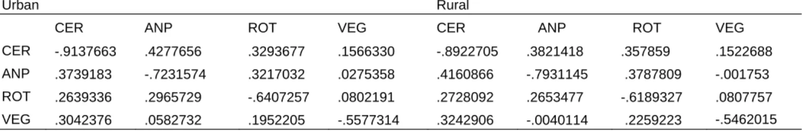
Table 5 gives estimates by area of the Hicksian elasticities which contain only price effects, contrary to the Marshallian elasticities which contain both income and price effects (Table A1). All

(13)

own-satisfied the negativity property. This is consistent with demand theory and suggests that the relationship between changes in price indexes and quantities demanded is inverse. The own-price elasticities suggest inelastic demand for all commodity groups analysed (elasticity absolutely < 1). Except for vegetable and animal products in rural areas, the remaining commodity groups carry positive signs for cross-price elasticity as expected for substitutable product. Cereals, and roots and tubers are identified as substitutes by households.

Table 5: Price elasticity from the QUAIDS model

Note: CER=cereals; ANP=animal products; ROT=roots and tubers; VEG=vegetables. Source: Authors’ computation from ECAM III.

3.3 Estimated impact of rising food prices on consumer welfare

Empirically, the CV can be seen here as a measure of the total transfer required for compensating households for a change in prices, as a percentage of their initial total food expenditure. The CV is disaggregating by area and poverty status in order to illustrate which groups of households are the most vulnerable to a price change. We utilize the estimated Hicksian elasticities to implement the CV as is usual in the literature (Ackah and Appleton 2007).

Following the CV framework, Equations (2) and (3) are used to estimate the impact of changing food prices on consumer welfare. We simulate the welfare impact of the increase in each commodity group by 10 per cent and 40 per cent in both the short and long run. Indeed, the analysis of food prices variation shows that on average in 2008, food prices have increased in the range of 10 per cent for fruit and vegetables and 40 per cent for cereals including imported ones such rice and maize (Medou 2008).

Tables 6 to 9 present long-run and short-run welfare effects of food price increases. One should note that in the short run, households cannot respond to price changes and thus, price elasticities are equal to zero.

Compensated/Hicksian elasticity

Urban Rural

CER ANP ROT VEG CER ANP ROT VEG

CER -.9137663 .4277656 .3293677 .1566330 -.8922705 .3821418 .357859 .1522688 ANP .3739183 -.7231574 .3217032 .0275358 .4160866 -.7931145 .3787809 -.001753 ROT .2639336 .2965729 -.6407257 .0802191 .2728092 .2653477 -.6189327 .0807757 VEG .3042376 .0582732 .1952205 -.5577314 .3242906 -.0040114 .2259223 -.5462015

(14)

Table 6: Compensating variation implied by change in cereals prices

Percentage increase in price 10% 40%

Short run Long run Short run Long run

Area Urban 2,44% 2,55% 9,75% 11,54% Rural 2,65% 2,77% 10,61% 12,51% Poverty status Non-poor 2,48% 2,59% 9,91% 11,71% Poor 2,82% 2,95% 11,29% 13,32%

Poverty status Rural Rural Rural Rural

Non-poor 2,60% 2,72% 10,40% 12,26%

Poor 2,79% 2,91% 11,16% 13,15%

Poverty status Urban Urban Urban Urban

Non-poor 2,40% 2,50% 9,58% 11,33%

Poor 2,92% 3,06% 11,69% 13,82%

Entire sample 2,61% 2,73% 10,43% 12,32%

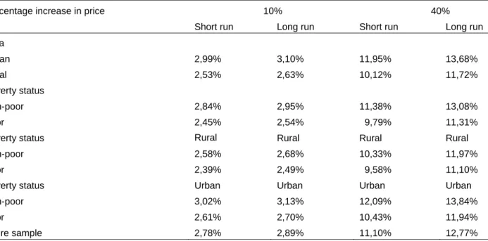
Table 7: Compensating variation implied by change in animal product prices

Non-poor 2,58% 2,68% 10,33% 11,97%

Poor 2,39% 2,49% 9,58% 11,10%

Non-poor 3,02% 3,13% 12,09% 13,84%

Poor 2,61% 2,70% 10,43% 11,94%

Entire sample 2,78% 2,89% 11,10% 12,77%

(15)

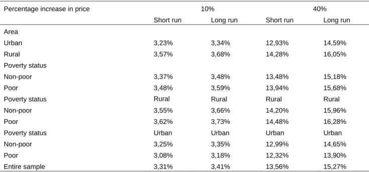
Table 8: Compensating variation implied by change in root and tuber prices

Non-poor 3,55% 3,66% 14,20% 15,96%

Poor 3,62% 3,73% 14,48% 16,28%

Non-poor 3,25% 3,35% 12,99% 14,65%

Poor 3,08% 3,18% 12,32% 13,90%

Entire sample 3,31% 3,41% 13,56% 15,27%

Table 9: Compensating variation implied by change in vegetable prices

Percentage increase in price 10% 40% Short run Long run Short run Long run

Non-poor 1,27% 1,30% 5,07% 5,62%

Poor 1,19% 1,23% 4,78% 5,30%

Non-poor 1,34% 1,37% 5,35% 5,94%

Poor 1,39% 1,43% 5,56% 6,18%

Entire sample 1,30% 1,34% 5,19% 5,76%

Results show that, on average, for each group of households there is a welfare loss due to the increase in food prices. However results reveal some heterogeneity in the welfare impact of food price volatility. Poor households in both urban and rural areas are the most affected as suggested in the literature (Ackah and Appleton 2007; Badolo and Traore 2012; Attanasio et al. 2013). For example, on average, poor households need to be reimbursed by about 15.68 per cent of their expenditure as the result of a 40 per cent change in the price of roots and tubers. We observe also that the highest welfare losses are due to increases in the price of roots and tubers. This is as expected since households spend more of their food budget on those commodities.

(16)

of the agricultural products they consume while poor urban households may not. On the other hand, it is the welfare of poor rural households that is most reduced due to an increase in the price of roots and tubers. Similar results were found by Leyaro (2009) and Ackah and Appleton (2007), whereas an increase in the price of animal products mostly affects the non-poor households in urban areas. This is in line with the fact that those households spend more of their total food budget on animal products.

The tables in this paper also show that the welfare effect of food price increases depends on the extent of the increases. Thus, there is an expected positive relationship between price increases and households’ welfare losses. They also show that the welfare effect in the long run is greater than in the short run.

4 Conclusion

This paper estimates the welfare impact of food price volatility in Cameroon. Using the QUAIDS model, we calculated expenditure, own-price and cross-price demand elasticities for the four main components of food consumption of most Cameroonian households. The results showed that demand for food commodities in Cameroon is price sensitive. In addition, poor households are, on average, the most affected by any hike in prices. However, welfare losses resulting from food price volatility is heterogeneous.

These results are important since it will be difficult to design efficient food policies without a thorough understanding of how different types of households in different areas are affected by changes in food prices and how sensitive they are. Having such information, policy makers will be able to implement more specific and efficient policies to fight against hunger and poverty in developing countries such as Cameroon. Nevertheless, even though such studies are important for developing countries, data constraints remain a major problem. For future research, it could be interesting to investigate how households are affected by changes in food prices using information on both producers and consumers.

(17)

Appendix

Table A1: Uncompensated/Marshallian elasticity from QUAIDS model

Note: CER=cereals; ANP=animal products; ROT=roots and tubers; VEG=vegetables

Urban Rural

CER ANP ROT VEG CER ANP ROT VEG

CER -1.149320 .1582713 .0358988 .0349649 -1.158581 .1375937 .0085518 .0271543 ANP .0707443 -1.070015 -.0560114 -.1290592 .1171294 -1.067641 -.0133482 -.1422051 ROT .0059980 .0014720 -.9620793 -.0530094 .0042896 .0187711 -.9711383 -.0453765 VEG .1179232 -.1548867 -.0369025 -.6539663 .096628 -.2130690 -.0726917 -.6531585

(18)

References

Ackah, C., and S. Appleton (2007). ‘Food Price Changes and Consumer Welfare in Ghana in the 1990s’. CREDIT Research Paper No. 07/03. Nottingham: University of Nottingham, Centre for Research in Economic Development and International Trade.

Attanasio, O., V. Di Maro, V. Lechene, and D. Phillips (2013). ‘Welfare Consequences of Food Prices Increases: Evidence from Rural Mexico’. Journal of Development Economics, 104: 136–51. Badolo, F., and F. Traore (2012). ‘Impact of Rising World Rice Prices on Poverty and Inequality

in Burkina Faso’. CERDI Working Paper E 2012.22. Clermont Ferrand: Centre d’Etudes et de Recherche sur le Développement International.

Banks, J., R. Blundell, and A. Lewbel (1997). ‘Quadratic Engle Curves and Consumer Demand’. Review of Economics and Statistics, 79: 527-39.

Barrett, C.B., and P.A. Dorosh (1996). ‘Welfare and Changing Food Prices: Nonparametric Evidence from Rice in Madagascar’. American Journal of Agricultural Economics, 78(3): 656–69. Béké, T.E. (2013). ‘Analysis of Substitutions in Demand for Food Crops in Ivory Coast’. Final

Report, CREA-AERC, processed, University F.H.B Cocody-Abidjan.

Bellemare, M.F., C.B. Barrett, and R. David (2010). ‘The Welfare Impacts of Commodity Price Fluctuations: Evidence from Rural Ethiopia’. Available at: http://economics.adelaide.edu.au/research/seminars/20130405-bellemare-barrett.pdf.

Accessed 12 June 2014.

Blein, R., and R. Longo (2009). ‘Food Price Volatility–How to Help Smallholder Farmers Manage Risk and Uncertainty’. Discussion Paper for IFAD’s Governing Council. Rome: IFAD. Cox, T., and M. Wohlgenant (1986). ‘Prices and Quality Effects in Cross-Sectional Demand

Analysis’. American Journal of Agricultural Economics, 68(4): 908–19.

De Janvry, A., and E. Sadoulet (2008). ‘Estimating the Effects of the Food Price Surge on the Welfare of the Poor’. UNDP/RBLAC, Poverty and MDG Cluster project.

De Janvry, A., and E. Sadoulet (2009). ‘The Impact of Rising Food Prices on Household Welfare in India’. IRLE Working Paper No. 192-09. Berkley, CA: Institute for Research on Labor and Employment, University of California.

Deaton, A. (1988). ‘Quality, Quantity and Spatial Variation of Price’. American Economic Reciew, 78: 418–30.

Deaton, A. (1989). ‘Rice Prices and Income Distribution in Thailand: a Non-parametric Analysis’. Economic Journal, 99 (395 Supplement): 1–37.

Deaton, A. (ed.) (1997). The Analysis of Household Surveys: a Microeconometric Approach to Development Policy. Baltimore: Johns Hopkins University Press.

Deaton, A., and J. Muellbauer (1980). ‘An Almost Ideal Demand System’. American Economic Review 70(3): 312–26.

FAO and OECD (2011). ‘Price Volatility in Food and Agricultural Markets: Policy Responses’. Policy Report. Paris: OECD.

Ferreira, F.H.G., A. Fruttero, P. Leite, and L. Lucchetti (2011). ‘Rising Food Prices and Household Welfare: Evidence from Brazil’. ECINEQ Working Paper No. 2011–200. Verona, Italy: Society for the Study of Inequality.

(19)

Friedman, J., and J. Levinsohn (2002). ‘The Distributional Impacts of Indonesia’s Financial Crisis on Household Welfare: A “Rapid Response” Methodology’. World Bank Economic Review 16: 397–423.

High Level Panel of Experts on Food security and Nutrition of the Committee on World Food Security (HLPE) (2011). ‘Price Volatility and Food Security’. A report by the High Level Panel of Experts on Food Security and Nutrition of the Committee on World Food Security. Rome: HLPE.

Leyaro, V. (2009). ‘Commodity Price Changes and Consumer Welfare in Tanzania in the 1990s and 2000s’. CREDIT Research Paper No. 10/01. Nottingham, UK: University of Nottingham, Centre for Research in Economic Development and International Trade. McKelvey, C. (2011). ‘Price, Unit Value, and Quality Demanded’. Journal of Development Economics,

95: 157–69.

Medou, J.C. (2008). ‘Evaluation de l’Impact de la Flambée des Prix des Denrées Alimentaires sur les Ménages dans les Milieux Urbains Camerounais’. World Food Programme, Ministry of Agriculture and Rural Development, Yaoundé: Cameroon.

Ministry of Economy, Planning, and Regional Planning (MINEPAT) (2008). ‘Autosuffisance et Sécurité Alimentaire au Cameroun: Une Analyse basée sur la Flambée des Prix des Produits Alimentaires de Première Nécessité’. Yaoundé: Cameroon.

Minot, N., and F. Goletti (2000). ‘Rice Market Liberalization and Poverty in Viet Nam’. IFPRI Research Report 114. Washington, DC: International Food Policy Research Institute.

National Institute of Statistics (NIS) (2008). ‘Conditions de Vie des Populations et Profil de Pauvreté au Cameroun en 2007’. ECAMIII Report. Yaoundé: Cameroon.

Niimi, Y. (2005). ‘An Analysis of Household Reponses to Price Shocks in Vietnam: Can Unit Values Substitute for Market Prices?’. Poverty Research Unit Working Paper 30. Brighton: University of Sussex.

Olorunfemi, S. (2013). ‘Demand for Food in Ondo State, Nigeria: Using Quadratic Almost Ideal Demand System’. Journal of Sustainable Development in Africa, 15(6): 16–45.

Poi, B.P. (2012). ‘Easy Demand-System Estimation with QUAIDS’. Stata Journal, 12(3): 433–46. Pollak, R.A., and T.J. Wales (1981). ‘Demographic Variables in Demand Analysis’. Econometrica, 49:

1533–51.

Pollak, R.A. and T.J. Wales (ed.) (1992). Demand System Specification and Estimation. New York: Oxford University Press.

Pons, N. (2011). ‘Food and Prices in India: Impact of Rising Food Prices on Welfare’. Delhi: Human Science Centre.

Ray, R. (1983). ‘Measuring the Cost of Children: an Alternative Approach’. Journal of Public Economics, 22: 89-102.

Tafere, K., S.A. Taffesse, S. Tamru, N. Tefera, and P. Zelekawork (2010). ‘Food Demand Elasticities in Ethiopia: Estimates Using Household Income Consumption Expenditure (HICE) Survey Data’. ESSP II Working Paper 11. Addis Ababa: IFPRI.

Turnovsky, S.J., S. Haim, and A. Schmitz (1980). ‘Consumer’sSurplus, Price Instability, Consumer Welfare’. Econometrica, 48(1): 135–52.