HAL Id: hal-01699301
https://hal.archives-ouvertes.fr/hal-01699301
Submitted on 2 Feb 2018
HAL is a multi-disciplinary open access
archive for the deposit and dissemination of
sci-entific research documents, whether they are
pub-lished or not. The documents may come from
teaching and research institutions in France or
abroad, or from public or private research centers.
L’archive ouverte pluridisciplinaire HAL, est
destinée au dépôt et à la diffusion de documents
scientifiques de niveau recherche, publiés ou non,
émanant des établissements d’enseignement et de
recherche français ou étrangers, des laboratoires
publics ou privés.
Let’s Be Lazy, We Have Time or, Lazy Reachability
Analysis for Timed Automata
Loïg Jezequel, Didier Lime
To cite this version:
Loïg Jezequel, Didier Lime. Let’s Be Lazy, We Have Time or, Lazy Reachability Analysis for Timed
Automata. 15th International Conference on Formal Modeling and Analysis of Timed Systems, Sep
2017, Berlin, Germany. �hal-01699301�
Let’s Be Lazy, We Have Time
or, Lazy Reachability Analysis for Timed Automata
Lo¨ıg Jezequel1and Didier Lime2
1 Universit´e de Nantes, LS2N UMR CNRS 6004
2 Ecole Centrale de Nantes, LS2N UMR CNRS 6004´
Abstract. In a recent work we proposed an algorithm for reachability analysis in distributed systems modeled as networks of automata. The main interest of this algorithm is that it performs its analysis in a lazy way: decision is done by only taking into account the automata poten-tially involved in a path to the reachability goal. This new work extends the approach to networks of timed automata, lazily considering the au-tomata but also lazily adding the clocks to the analysis, which implies not only to consider clocks tested along the paths to the goal, but also to deal with the special issues due to urgency and shared clocks. We have implemented our approach as a tool and provide some interesting experimental results, in a comparison with the model-checker Uppaal.
1
Introduction
The verification of concurrent timed systems is a crucial and challenging issue. It is subject to both an explosion of the number of discrete states due to the number of concurrent components, and an explosion of the clock space due to the number of clocks.
To model such systems we focus here on networks of timed automata and the verificaion of reachability properties. Since the seminal article of Alur and Dill establishing the PSPACE completeness of this problem [1], many techniques have been developed to improve the practical efficiency of reachability verification.
Efficient symbolic representations of the clock space have been proposed, implemented using a data structure called Difference Bound Matrix [5, 7], as well as efficient algorithms to handle them [16]. Different kind of abstractions have then been devised to further improve them [2, 12].
Better exploration orders [13] have also been proposed and quite a few au-thors have defined partial-order reductions for timed automata (see e.g. [10, 18, 6] and the references therein). Some decision-diagram-based representations of the state-space have also been proposed [15, 20]. Several tools are available that implement part of these techniques, this is in particular the case of Uppaal [17]. In this article, we exploit a technique orthogonal to most of those mentioned above and build on a recently proposed lazy reachability analysis algorithm in compound systems modeled as networks of labelled transition systems [14], that
we extend to the timed setting. The resulting algorithm can be implemented using the successful DBM data structure. It starts separately from each of the components explicitly mentioned in the reachability property and adds other components, as well as clocks, on demand, based on the analysis of the successive overapproximations obtained by ignoring some components or clocks. Since we start by verifying separately that each component in the property can indeed reach its goal, the algorithm also performs synchronisations to make sure that in reaching its goal, one component does not prevent another one to do so.
The timed setting brings a few difficulties of its own, namely: choosing the clocks to add, handling urgency, and accounting for shared clocks. It can be proven that our algorithm is sound, complete and that it terminates. We pro-vide a rather naive prototype implementation that nonetheless produce some interesting experimental results.
This paper is organized as follows. In Section 2 we recall basic definitions about timed automata, give some definitions and notations about compound systems built from timed automata, and we define the reachability problem we consider. In Section 3 we briefly recall the lazy reachability algorithm of [14] and we describe the modifications needed to make it cope with timed systems. In Section 4 we discuss an implementation of this algorithm as a publicly avail-able tool: LaRA-T and we present an experimental evaluation, comparing its performances to those of Uppaal on a few classic examples.
2
Definitions
In this section we first recall standard definitions for timed automata and set the notations we use in the paper. Then, we define the reachability problem on compound systems built from timed automata that we aim at solving.
2.1 Timed automata
Definition 1 (Clocks, clock constraints). Let X be a set of real-valued vari-ables called clocks. A clock constraint over X is a constraint of the form x ∼ k with x ∈ X, k ∈ N, and ∼∈ {<, ≤, =, ≥, >}. The set of all possible such clock constraints over X is denoted by B(X). The subset of B(X) where ∼∈ {<, ≤} is denoted by B0(X).
For simplicity, we do not consider clock differences in the above defined con-straints. The high level algorithm presented in this paper is however independant of the exact reachability analysis technique used, so our approach is not restricted to these simple constraints.
Definition 2 (Clock valuations). For a set of clocks X we call clock valu-ation a function v : X → R≥0 associating a non-negative real number to each
clock in X. We denote by V (X) the set of all such valuations. Given a subset R of X and a clock valuation v, we denote by v[R] the clock valuation such that ∀x ∈ R, v[R](x) = 0 and ∀x /∈ R, v[R](x) = v(x). Given d ∈ R≥0, we denote by
Definition 3 (Constraint satisfaction). A clock valuation v satisfies a con-straint b = x ∼ k, written v |= b, if and only if v(x) ∼ k. A clock valuation v satisfies a set of constraints g, written v |= g, if and only if it satisfies each of its elements.
In this article, we consider timed automata with invariants [11]. Finite au-tomata are extended with clocks that can be tested in guards to allow some transition to be taken, and can also be reset to 0 when some transition is taken. Invariants further specify constraints on clocks that must be satisfied to stay or enter in a given location. They add a notion of urgency to the timed automata of [1].
Definition 4 (Timed automata: syntax). A Timed automaton (TA) is a tuple A = (L, `0, Σ, X, E, Inv) where L is a set of locations, `0∈ L is an initial
location, Σ is a set of action labels, X is a set of clocks, E ⊆ L × 2B(X)× Σ × 2X× L is a set of transitions, and Inv : L → 2B0(X)
associates invariants to the locations.
In the rest of the paper A will denote the tuple (L, `0, Σ, X, E, Inv). Simi-larly, A0 will denote the tuple (L0, `00, Σ0, X0, E0, Inv0). And, for any i, A
i will
denote the tuple (Li, `0i, Σi, Xi, Ei, Invi). For a transition e = (`, g, σ, R, `0) ∈ E,
we note `(e) = `, g(e) = g, σ(e) = σ, R(e) = R, and `0(e) = `0. Moreover, Σ(A) = {σ ∈ Σ : ∃e ∈ E, σ(e) = σ} denotes the set of actions actually used by A. Similarly, X(A) = {x ∈ X : ∃e ∈ E, g(e) ∩ B({x}) 6= ∅ ∨ x ∈ R(e)} ∪ {x ∈ X : ∃` ∈ L, Inv(`) ∩ B({x}) 6= ∅} denotes the set of clocks actually appearing in A. And finally, Res(A) = {x ∈ X : ∃(`, g, σ, R, `0) ∈ E, x ∈ R} denotes the set of clocks reset by A.
A state of a timed automaton consists of a location, and a value for each of its clocks. The state of a timed automaton evolves either by letting time pass, or by taking a transition. This is formalised in the following definition:
Definition 5 (Timed automata: semantics, timed-paths, timed-runs, reachable locations, duration). A state of a timed automaton A is a pair (`, v) ∈ L × V (X) so that v |= Inv(`). A transition relation →A is defined over
the states of A as follows: (`, v) →A(`0, v0) if and only if:
– ` = `0 and ∃d ∈ R≥0 so that v0 = (v + d) (time elapsing of duration d), or
– ∃e ∈ E, such that `(e) = `, `0(e) = `0, v |= g(e), and v0 = v[R(e)] (discrete transition firing – of duration 0).
A finite timed-path (or simply, path) of A is a sequence (`0, v0) . . . (`n, vn) of
states such that ∀i ∈ {0..n − 1}, (`i, vi) →A (`i+1, vi+1). If, moreover, `0 = `0
(i.e `0 is the initial location of A), we call (`0, v0) . . . (`n, vn) a finite timed-run
(or simply, run) of A. When there exists such a run, we say that `n is reachable
in A. The duration of a timed-path is the sum of the durations of its transitions. In the rest of the paper we denote by Urg(A) the set of initially urgent locations of A. These locations are the ones appearing on a timed-run so that
any location in it has a non-empty invariant. Formally, Urg(A) is the smallest set such that (a) if Inv(`0) 6= ∅ then `0 ∈ Urg(A), and (b) if e ∈ E with `(e) ∈ Urg(A) and Inv(`0(e)) 6= ∅ then `0(e) ∈ Urg(A).
And we denote by Req(A) the set of actions that could be requested by A due to urgency: the actions appearing in transitions originating from locations in Urg(A). Formally, Req(A) = {σ ∈ Σ : ∃e ∈ E, σ(e) = σ ∧ `(e) ∈ Urg(A)}.
2.2 Reachability problem in compound systems
We are interested in systems made of several interacting components. To for-malise this notion, we define compound systems.
Definition 6 (Compound system). Let A1, . . . , An be TAs. The compound
system A1|| . . . ||An is the TA A such that:
– L = L1× . . . × Ln, `0= (`01, . . . , `0n), Σ = Σ1∪ . . . ∪ Σn, X = X1∪ . . . ∪ Xn,
– ((`1, . . . , `n), g1∪ . . . ∪ gn, σ, R1∪ . . . ∪ Rn, (`01, . . . , `0n)) ∈ E if and only if
∀i ∈ [1..n]:
• σ ∈ Σi implies (`i, gi, σ, Ri, `0i) ∈ Ei, and
• σ /∈ Σi implies `i= `0i, gi= ∅, and Ri= ∅,
– ∀` = (`1, . . . , `n) ∈ L, Inv(`) = Inv1(`1) ∪ . . . ∪ Invn(`n).
Definition 7 (Time-non blocking timed automaton). A timed automaton A is time-non blocking if, in any state and for any duration d, there exists a finite timed-path from that state with duration d.
In all this article, we assume that compound systems are time-non blocking TA. Else, an invariant of any TA could block the whole system. This would force to always consider all the TA of a system to perform reachability analysis.
The next definitions allow us to specify reachability objectives related to only a part of the global system.
Definition 8 (Global locations, partial locations, concretisation). In a compound system A1|| . . . ||An we call any element from L1× . . . × Ln a global
location. We call partial location any element from (L1∪ {?}) × . . . × (Ln∪
{?}) \ {(?, . . . , ?)}, where ? is a special symbol not in any Li. We say that a
global location (`01, . . . , `0n) concretises the partial location (`1, . . . , `n) if and only
if ∀i ∈ [1..n], `i6= ? implies `0i= `i.
Definition 9 (Reachability problem). In a compound system A we say that a partial location ` is reachable (in A) if and only if there exists a global location that (1) is reachable in A and (2) concretises `. Given a set R of partial locations, we call reachability problem the problem of deciding if there exists a reachable element in R. We denote this problem by RPAR.
In this paper, we propose a lazy backtracking-based algorithm for solving such reachability problems. We avoid as much as possible to compute the full compound systems considered, only taking into account the subsets of their components and clocks that are needed for reachability analysis. In the remaining of this section we introduce a few more definitions, simplifying the description of our algorithm.
2.3 Partial compound systems
The following definitions allow us to reason about only parts of the global system, be they obtained by considering only some of the components, some of the clocks, or even a partial behaviour of some components.
Definition 10 (Isomorphic timed automata). Let A1 and A2 be two TA.
We say that they are isomorphic if and only if Σ1 = Σ2, X1 = X2, and there
exists a bijection f : L1→ L2 so that: f (`01) = `02, (`, g, σ, R, `0) ∈ E1if and only
if (f (`), g, σ, R, f (`0)) ∈ E2 and ∀` ∈ L1, Inv1(`) = Inv2(f (`)).
Definition 11 (Neutral element). We denote by Aid the TA such that Lid=
{id}, `0
id = id, Σid = ∅, Xid = ∅, Eid = ∅, and Invid(id) = ∅. As, for any TA
A, A||Aid is isomorphic to A, Aid can be considered as the neutral element for
the composition of TAs. For any TA A we denote by id(A) the TA whose only location is the initial location of A and which is isomorphic to Aid.
Definition 12 (Clock projection). For a TA A and a set of clocks X0, we denote by PX0(A) the TA A0 so that: L0= L, `00 = `0, Σ0= Σ, X0 is the set of
clocks, E0 = {(`, g ∩ B(X0), σ, R ∩ X0, `0) : (`, g, σ, R, `0) ∈ E}, Inv0 is so that ∀` ∈ L, Inv0(`) = Inv(`) ∩ B(X0).
Definition 13 (Extensions). A TA A1 extends a TA A02, noted A1 w A02,
if and only if A02 is isomorphic to some TA A2 so that: L2 ⊆ L1, `02 = `01,
Σ2 ⊆ Σ1, X2 = X1, E2 ⊆ E1|L2,Σ2, Inv2 = Inv1|L2, with E1|L2,Σ2 = {e ∈
E1 : `(e), `0(e) ∈ L2∧ σ(e) ∈ Σ2} and Inv1|L2 the function defined over L2
and so that ∀` ∈ L2, Inv1|L2(`) = Inv1(`). If moreover at least one of the above
inclusions is strict, we say that A1 strictly extends A02, which we note A1A A02.
Definition 14 (Initialisation). For a TA A and a set of clocks X0 we denote by ini(A, X0) the TA with the same locations, initial location, and transitions as id(A) but with X0 as set of clocks, the same set of actions as A, and the same invariants as A on its initial location. Notice that PX0(A) w ini(A, X0).
Definition 15 (Partial compound system). A TA A0 is a partial com-pound system of A = A1|| . . . ||An if there exist m TAs A0k1, . . . , A
0 km with
{k1, . . . , km} ⊆ [1..n], such that A0 = A0k1|| . . . ||A 0
km and PX0ki(Aki) w A 0 ki
for all i in [1..m].
In the rest of this paper, for a compound system A = A1|| . . . ||An, a partial
compound system A0 = A0k
1|| . . . ||A 0
km of A, the set K = {k1, . . . , km}, and a
set R of partial locations of A, we adopt the following notations.
By A0 → R|K we denote that R is (partially) reachable in A0. That is, the
fact that there exists a location from R|K = {(`0k1, . . . , ` 0
km) : ∃(`1, . . . , `n) ∈
R, ∀i ∈ [1..n], ∀j ∈ [1..m], i = kj ⇔ `i= `0kj} which is reachable in A 0.
By Conf(A0, K) we denote the set of actions in conflict with A0with respect to K: the actions from AK= Ak1|| . . . ||Akmoriginating from locations in L
0but not
appearing in transitions from E0. Formally Conf(A0, K) = {σ /∈ Σ(A0) : ∃e K ∈
EK, σ(eK) = σ ∧ `(eK) ∈ L0} (assuming not only isomorphism but equality in
3
From lazy reachability to lazy reachability with time
In this section we give an as generic as possible description of our lazy reachabil-ity algorithm. This description is strongly based on what we proposed recently for non-timed systems [14]. We show that it extends naturally to timed-systems. This however implies non-trivial modifications, in particular to handle invari-ants and resets of shared clocks. These modifications mostly impact the notion of completeness, which is the main notion behind the validity of the approach.
3.1 Introductory example
The main goal of our algorithm is to be as lazy as possible when solving a reach-ability problem in a compound system. That is, trying to involve the smallest number of automata and the smallest number of clocks of these automata in the reachability analysis. In order to get an overview of our approach to do so, lets consider the example of Figure 1.
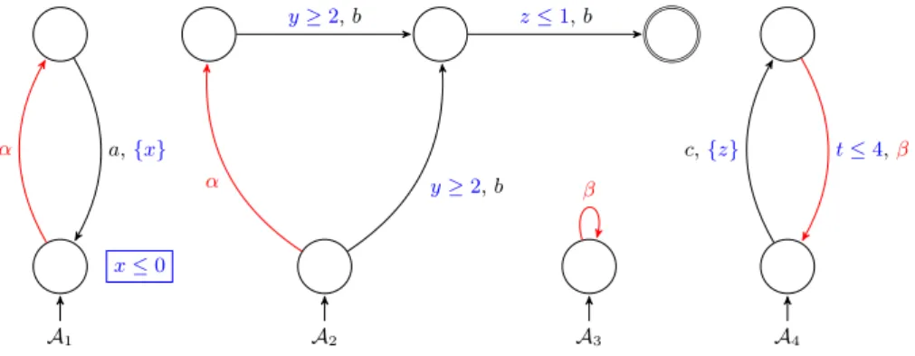
A1 x ≤ 0 α a,{x} A2 α y ≥ 2, b y ≥ 2, b z ≤ 1, b A3 β A4 c,{z} t ≤ 4,β
Fig. 1. A compound system involving four timed automata.
This figure shows a compound system made of four TAs: A1, A2, A3, and
A4. Locations are depicted as circles and transitions as arrows with labels
indi-cating guards, actions, and clocks resets (in this order, with empty guards and empty sets of resets omitted). Initial locations are the ones with input arrows coming from no other location. Invariants are depicted in rectangles near the corresponding locations (there is only one invariant, in A1, in this figure). There
are three interactions in this system: A1 interacts with A2 because they share
theα action, A2 interacts with A4 because they share thez clock, and A3
in-teracts with A4 because they share theβ action. The objective here is to reach
the double circled location in A2.
One can start from a partial compound system P∅(A2), and look for a path
to the objective. A possibility is bb. The clock constraints have to be added, moving to a partial compound system A2. The constraint y ≥ 2 for the first b
can be satisfied by waiting for (at least) 2 time units. After that, the constraint
z ≤ 1for the second b cannot be fulfilled. However,zis a clock that can be reset by A4. One thus adds P{z}(A4) to the partial compound system. It appears that
bcb allows to reach the objective, fulfilling all the timing constraints.
However, in A2, the first b is in conflict with α. Andα is shared with A1,
where it has to be used with no delay, due to the invariant x ≤ 0. This im-mediately discards bcb as a possible path to the reachability objective in the global compound system. One thus, looks for another path to the objective in A2||P{z}(A4).
A possibility is αbcb. This immediately implies to add A1 to the partial
compound system because of the shared action α. In the partial compound system A1||A2||P{z}(A4),αbb is clearly a timed-run. It can be verified that this
run is also a run of the global compound system.
Using this incremental process, one has found a way to satisfy the reachability objective. This has been done without considering the automaton A3, nor the
clock t. This is why we call our algorithm lazy. The remainder of this section formalizes the approach we just exemplified.
3.2 General scheme of the algorithm
Algorithm 1 presents the general scheme of our algorithm3. This algorithm starts
from a partition of the TAs involved in the reachability objective. The idea is to verify this objective separately on each involved component, with the hope to find a solution involving no interaction between these components. The current state of the search is stored in the list Ls which has initially one element per part of the initial partition. Each such element is a list of tuples (A, C, I, J, K, L, M ) – described in details in the next subsection – that represent more and more concrete partial compound systems: they include more and more automata and take into account more and more clocks. The more concrete partial compound system is at the head of the list.
First note that the initial partition of the TAs has to be well-formed (line 1), by that we mean that it should contain only one element I1= Lgif any TA has
an invariant on a reachability objective (that is ∃i ∈ Lg, ∃(`1, . . . , `n) ∈ R, so
that `i6= ? and Invi(`i) 6= ∅).
Each element in the initial partition has to be completed with all automata resetting some clocks of the automata in that element (lines 3,4). Resetting a clock may indeed add some behaviours, which could be overlooked otherwise.
After initialising Ls, we proceed to the main loop, which consists of two oper-ations: concretisation, ensuring completeness, and merging, ensuring consistency. These notions and functions are described in the following subsections.
3 Notice that the algorithms presented in this paper make use of the classic abstract
list data-structure. The usual operations hd(), tl(), and len() give respectively the head, tail, and length (number of elements) of a list. The list constructor (prepend) is denoted by : and the list concatenation is denoted by ++ . The rev() operator reverses a list. The empty list is denoted by [ ]. Finally, L[i] denotes the ithelement
Algorithm 1 Algorithm solving RPAR (Lg: indices of TAs involved in R)
1 choose anywell-formed partition {I1, . . . , Ip} of Lg
2 for all kin [1..p] { 3 let Ik0 = Ik
4 until stability let Ik0 = Ik0 ∪ {i /∈ Ik0 : ∃j ∈ Ik0, Res(Ai) ∩ X(Aj) 6= ∅}
5 let IDk= ||i∈I0kid(Ai)
6 let INIk= ||i∈I0
kini(Ai, ∅)
7 }
8 let Ls = [[(ID1, INI1, I1, ∅, I10, ∅, ∅)], . . . , [(IDp, INIp, Ip, ∅, Ip0, ∅, ∅)]]
9 let Complete =false 10 let Consistent = false
11 while notCompleteor notConsistent { 12 let Complete = IsComplete(Ls) 13 if notComplete {
14 optional unlessConsistent {
15 if notConcretise(Ls) {returnfalse}
16 }
17 }
18 let Consistent = IsConsistent(Ls) 19 if notConsistent {
20 optional unlessComplete { Merge(Ls) } 21 }
22 }
23 returntrue
3.3 Completeness, concretisation and the Concretise function
The main loop of Algorithm 1 iterates as long as the current state Ls of the search is not complete. We say that Ls is complete (noted IsComplete(Ls)) if and only if, for any indice k, Ls[k] is complete. Intuitively, this means that the partial compound system represented by hd(Ls[k]) contains a path to reach the corresponding local goal. Moreover, this path has to (1) use no action of any automaton not participating in this partial compound system, (2) have no conflict with actions that could be externally forced by an invariant (this was the case of action αin the above example), (3) avoid relying on the satisfaction of a clock constraint involving a clock that is reset by an automaton not from this partial compound system (this was the case of clock z in the above example), and (4) take into account all clock constraints on any transition involved. In other words: a partial compound system is complete if it can reach a local goal alone.
In any tuple (A, C, I, J, K, L, M ), in particular in hd(Ls[k]), C is the TA representation of the partial compound system considered, and J ∪ K contains the indices of the TAs (from the global compound system) involved in this partial compound system. The above notion of completeness can be formalized from only C, J , and K. The other elements of the tuple are instrumental for building our
algorithm and are described later. In the following definition of completeness, points (1-4) correspond to intuitions (1-4) above.
Definition 16 (Completeness). The list Ls[k] so that hd(Ls[k]) = (A, C, I, J, K, L, M ) is complete if ∃C∗ so that: C w C∗, C∗ → R|J∪K, and (1) ∀i /∈
J ∪K, Σi∩Σ(C∗) = ∅, (2) ∀i /∈ J ∪K, Conf(C∗, J ∪K)∩Req(Ai) = ∅ (3) ∀i /∈ J ∪
K, Res(Ai) ∩ X(C∗) = ∅ (4) {x /∈ X(C∗) : ∃A∗, ||i∈J ∪KAiw A∗, PX(C∗)(A∗) =
C∗, x ∈ X(A∗)} = ∅.
In order to achieve completeness, we use the Concretise function defined in Algorithm 2. This is basically a standard backtracking algorithm, specialized for incrementally building more and more concrete partial compound systems: partial compound systems containing (1) more and more states and transitions, for a fixed set of TAs and clocks, and (2) more and more TAs and clocks.
Algorithm 2 Auxiliary function Concretise(Ls) for Algorithm 1
1 choose anykin[0..len(Ls) − 1]such that notIsComplete(Ls[k]) 2 let (A, C, I, J, K, L, M ) = hd(Ls[k])
3 let Back = tl(Ls[k])
4 if ∃C∗ s.t. (||i∈KPL∪M(Ai))||A w C∗A C andC∗→ R|J ∪K {
5 choose any suchC∗
6 let NA= {i /∈ J ∪ K : Σi∩ Σ(C∗) 6= ∅}
7 let A0 be such that||i∈J ∪KAiw A0andP∅(A0) = P∅(C∗)
8 let NX= {x /∈ L ∪ M : x ∈ X(A0)}
9 caseNA∪ NX6= ∅
10 choose anyK0, M0 such thatK0⊆ NAandM0⊆ NX andK0∪ M06= ∅
11 let Back0= (A, C∗, I, J, K, L, M ) : Back 12 let J0= J ∪ K
13 let L0= L ∪ M 14 let K00= K0
15 until stability let K00= {i /∈ J0∪ K00 : ∃j ∈ K00, Res(Ai) ∩ X(Aj) 6= ∅}
16 let A∗ be such that||i∈J ∪KPL0∪M0(Ai) w A∗andP∅(A∗) = P∅(C∗)
17 let Ls[k] = (A∗, ||i∈J0∪K00ini(Ai, L0∪ M0), I, J0, K00, L0, M0) : Back0
18 caseN = ∅
19 let Ls[k] = (A, C∗, I, J, K, L, M ) : Back 20 }else {
21 if Back = [ ] { returnfalse} 22 else {let Ls[k] = Back } 23 }
24 returntrue
The list Ls[k] contains the search history: backtracking means replacing this list by its tail (else part of the conditional at line 4). Notice that, when back-tracking, it could be possible to allow to remember the unsuccessful searches (this can be used for speeding up the future searches). This has been described in [14] for un-timed systems.
Any element of Ls[k], and in particular the one reflecting the current state of the search (the head of Ls[k]), is a tuple (A, C, I, J, K, L, M ) where: A is the partial compound system computed at the previous call to Concretise, C is the current partial compound system we consider, I gives the initial partition of TAs involved in the objective, J gives the TAs involved in A, K gives the TAs that can be used to build C from A, L gives the clocks involved in A, and M gives the clocks that are used to build C from A.
The main idea of the function consists in first choosing a partial compound system C∗ bigger than what we already had, and that can reach the goal. Set NA then corresponds to the automata sharing some action with C∗, but not
added, and NX to the clocks tested, but not present, in C∗. From these sets, we
can choose automata or clocks to add to our partial compound system in order to try to make it complete (line 10). The next lines create the new tuple that will be put at the head of Ls as the new current level of concretisation (line 17), to reflect these choices. Line 15 forces the addition of automata that reset some clocks we have chosen to add. This is important because resetting a clock may add some new behaviours. Finally, A∗(line 16) is a version of C∗with the whole set of clocks we have up to now (those we already had and those we have just chosen to add). It will serve as an upper bound (wrt. w) for the choice of C∗ at the next level of concretisation. Note that at this next level we start with a partial compound system reduced to the initial states of the chosen automata (and with all the chosen clocks). If we have no clocks or automata to add from NX, NA, then we simply update the current partial compound with C∗(line 19)
and back in the main algorithm we will check if this has allowed us to achieve completeness (line 11 of Algorithm 1). If we could not find C∗ at all, then it is not possible to reach the goal with the current upper bound an we need to backtrack to extend this upper bound at a lower level of concretisation, i.e., with fewer clocks or automata (line 22).
3.4 Consistency, merging and the Merge function
Achieving completeness for each element of Ls is not sufficient however to solve our reachability problem. Indeed, it may be the case that some automata ap-pear in several different elements of Ls: we start from a partition but the same automata may be added to elements of Ls during concretisation steps. In this case, it is likely that some paths in different partial compound systems interfere: they use the same actions but not in the same order or they need incompatible valuations of the clocks for satisfying clock constraints. The main loop of Algo-rithm 1 reflects this by iterating as long as the current state Ls of the search is not complete, as explained above, or not consistent.
Definition 17 (Consistency). Ls = [(A1, C1, I1, J1, K1, L1, M1) : Back1, . . . ,
(An, Cn, In, Jn, Kn, Ln, Mn) : Backn] is consistent if ∀i 6= j ∈ [1..n], (Ji∪ Ki) ∩
(Jj∪ Kj) = ∅.
In order to achieve consistency we use a Merge function to replace two elements of Ls: Ls[i] (with hd(Ls[i]) = (Ai, Ci, Ii, Ji, Ki, Li, Mi) and tl(Ls[i]) =
Backi) and Ls[j] (with hd(Ls[j]) = (Aj, Cj, Ij, Jj, Kj, Lj, Mj) and tl(Ls[j]) =
Backj) by a single one h : Back obtained by merging them, thus reducing
the length of Ls by one. The simplest such new element would be such that: Back = [ ] and h = (IDi||IDj, INIi||INIj, Ii ∪ Ij, ∅, Ii0 ∪ Ij0, ∅, ∅). However, it
may be of interest to use the current state of the search in both Ls[i] and Ls[j], taking instead: Back = [(IDi||IDj, INIi||INIj, Ii∪ Ij, ∅, Ii0∪ Ij0, ∅, ∅)], and
h = (PLj(Ai)||PLi(Aj), PLj∪Mj(Ci)||PLi∪Mi(Cj), Ii∪ Ij, Ji∪ Jj, Ki∪ Kj).
In fact, it is even possible to replace Ls[i] and Ls[j] by any history that could have been produced by a sequence of call to Concretise starting from (IDi||IDj, INIi||INIj, Ii∪ Ij, ∅, Ii0 ∪ Ij0, ∅, ∅) (of which the two above examples
are particular cases). This avoids to un-merge when backtracking, has been for-malized as a notion of good Merge in our previous work [14], and remains essentially the same for timed systems.
3.5 Termination, soundness, completeness
Theorem 1 explicits the fact that Algorithm 1 always terminates, and is sound and complete. Due to space limitations, its proof is omitted.
Theorem 1. Algorithm 1 always terminates. It returns true if and only if the goal is reachable.
3.6 Example
We get back to the introductory example and see how our algorithm may find the result we intuitively outlined.
First we choose an initial partition of the automata directly involved in the objective. Here there is only A2so Ls = [(id(A2)||id(A4), ini(A2, ∅)||ini(A4, ∅),
{2}, ∅, {2, 4}, ∅, ∅)]. Note in particular that I0
1= {2, 4} because clock z is present
in A2 and reset by A4. Also, since we have only one element in our partition,
we will always stay consistent in this example.
Now we can call Concretise and choose k = 0 (the only possibility). We choose for instance C∗ as the compound system C24 made of the path bb in
A2 and the path c in A4, which permits to reach the goal. Then NA = ∅
and NX = {y, z}. We can now choose K0 = ∅ and M0 = {y, z} for instance.
Then K00 = ∅. Finally, A∗ is C∗ = C24 augmented by the clocks y and z,
slightly abusing notations we denote it by P{y,z}(C24). The function returns true,
and Ls[0] = [Ls1, Ls00] with Ls00= (id(A2)||id(A2), C24, {2}, ∅, {2, 4}, ∅, ∅)], and
Ls1= (P{y,z}(C24), ini(A2, {y, z})||ini(A4, {y, z}), {2}, {2, 4}, ∅, ∅, {y, z}).
Back in the main algorithm, starting from ini(A2, {y, z})||ini(A4, {y, z})
we obviously do not have completeness. So we call Concretise again. We choose, for instance C∗as the full P{y,z}(C24), in which the goal can be reached.
Both NA and NX are empty, so we proceed to line 19 and Ls[0] becomes
[(P{y,z}(C24), P{y,z}(C24), {2}, {2, 4}, ∅, ∅, {y, z}), Ls00]. We return true.
Back in the main algorithm, P{y,z}(C24) is not complete because α is in
Definition 16) so we need to call Concretise again. There, we have to choose something strictly bigger than the C, i.e P{y,z}(C24), which is not possible with
K being empty. We reach line 22 (backtracking) and Ls[0] becomes [Ls00]. In the main algorithm again, Ls is not complete because C24 (the C value
of Ls00) is not complete (for the same conflict with α as above). We choose to add the rest of A2and choose therefore C∗ as the compound system C240 made
of A2 and the path c of A4. Then NA = {1} because α is shared with A1 and
NX = {y, z}. We choose K0 = {1}, M0= ∅ and since we have no further shared
clock, we have K00= K0. Since we have not added clocks, A∗= C240 and finally Ls[0] becomes [Ls01, Ls000] with Ls000 = (id(A2)||id(A4), C240 , {2}, ∅, {2, 4}, ∅, ∅),
and Ls01 = (C240 , ini(A1, ∅)||ini(A2, ∅)||ini(A4, ∅), {2}, {2, 4}, {1}, ∅, ∅). We
re-turn true.
Back in the main algorithm we are not complete since we do not reach the goal in ini(A1, ∅)||ini(A2, ∅)||ini(A4, ∅) so we call Concretise. We choose for
instance C∗as the compound system C
124 made of the path α in A1, the whole
of A2 and the path c in A4. Then NA= ∅ but NX = {x, y, z} because clock x
is tested in the invariant of A1. So we have to choose K0= ∅ and decide to take
M0 = {x, y, z}. We have K00= K0. Hence, A∗ is C124 augmented by the clocks
x, y and z, slightly abusing notations we denote it by P{x,y,z}(C124). And Ls[0]
becomes [Ls2, Ls001, Ls000], with Ls001 = (C240 , C124, {2}, {2, 4}, {1}, ∅, ∅) and Ls2=
(P{x,y,z}(C124), ini(A1, {x, y, z}) || ini(A2, {x, y, z}) || ini(A4, {x, y, z}), {2},
{1, 2, 4}, ∅, ∅, {x, y, z}). We return true.
Again in the main algorithm we are not complete because we do not reach the goal in the C value of Ls2, so we call Concretise. We choose C∗ as the
com-pound system C1240 made of the path α in A1(but with x this time), the whole of
A2(with y and z this time ) and the path c in A4(with z this time). Now taking
into account the clocks C0
124 does allow to reach the goal, but only through the
path αbcb. Furthermore, NX= NA= ∅ so we proceed to line 19 and Ls[0] is now
[Ls02, Ls001, Ls000], with Ls02= (P{x,y,z}(C124), C1240 , {2}, {1, 2, 4}, ∅, ∅, {x, y, z}). We
return true. Finally, the main algorithm concludes that C1240 is complete and ter-minate, by concluding that the goal is indeed reachable.
4
Experimental analysis
We implemented an instance of the above algorithm as a tool called LaRA-T. The LaRA-T tool represents around 2000 lines of code written in the func-tional language Haskell4. It is built over the previous LaRA tool for reachabil-ity analysis in networks of (untimed) automata [14]. Both tools are available for download5.
The algorithm we have presented is very general and the current implemen-tation results from some important choices. First, each time we add automata or clocks, we compute the resulting partial compound system completely. This
4 https://www.haskell.org/ 5
eliminates the need for backtracking, since if we cannot find the goal in this par-tial compound system then it is for sure not reachable at all. In that respect, this choice also heuristically favors the unreachable case. Second, we only compute the reachable parts of the compound systems, using a classic DBM-based sym-bolic state exploration [16], with DBM inclusion checking and maximal constant per clock extrapolation. Finally, when we have computed a whole partial com-pound system, we look at the paths we have followed to reach all goal states. If some automata or clocks are required for completeness with respect to all those paths, then we add them all at the next level. Otherwise, we add one arbitrary required automaton or clock with the following priority: first automata ((1) of Definition 16), then clocks actually used on some path to the goal (4), and fi-nally clocks coming from urgent conflicts due to invariants (2). We have not yet implemented the support for shared clocks (hence (3) of Def. 16 not appearing in the previous priority order).
We compared LaRA-T to Uppaal [4] on several examples from the literature on analysis and verification of timed systems6:
CritReg is a modeling of a critical region protocol from PAT [19] benchmarks. We check the reachability of an error location in one of the automata. This is a true property.
Fddi is a modeling of a communication protocol based on a token ring network presented in [9] and adapted to our setting in [13]. We check the reachability of a couple of mutually exclusive locations. This is a false property.
Fischer is a modeling of Fischer’s mutual exclusion protocol [3]. We check the reachability of a couple of mutually exclusive locations. This is a false property.
Fischer2 is a variation of Fischer’s mutual exclusion protocol where a time constant has been changed, breaking the mutual exclusion guarantee. In this example, the property is true.
Trains1 is the Train model of Uppaal [3]. A controller is responsible for a queue of trains and has to prevent more than one of them to access a bridge together. We check the reachability of a state in which the two first trains are crossing the bridge at the same time. This is a false property.
Trains2 is a variation of the Trains1 benchmark where the controller manages a set of trains rather than a queue of trains.
Trains3 is a model where a railway crosses a road [8]. A controller has to ensure that the gate is closed (cars cannot crosse the railway) as soon as a train crosses the road. We check the reachability of a state in which a train crosses the road while the gate is open. This is a false property.
4.1 Experimental results
For each example we ran Uppaal and LaRA-T on instances of growing size (the size is, roughly, the number of timed-automata, see Table 2 for precise
6
information), with a time-limit of 20 minutes at each size. In order to better evaluate the performances of the laziness mechanism (independently of our im-plementation of the DMB-based computation of the state-space of a TA) we also ran LaRA-T with all components and clocks in a single element of the initial partition (LaRA-T Full). All the experiments were run on the same ma-chine with four Intel R Xeon R E5-2620 processors (six cores each) with 128GB
of memory. Though this machine has some potential for parallel computing, all the experiments presented here are actually monothreaded.
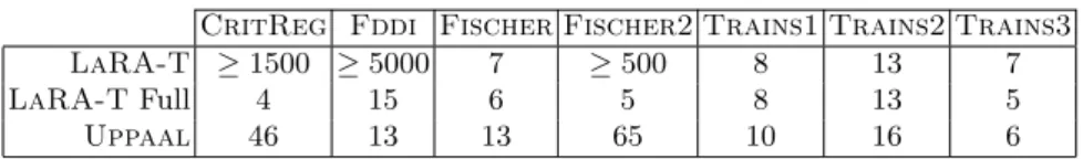
Table 1 gives the largest instance of each example solved by each tool within the time-limit.
Table 1. Size of last instances solved within 20 minutes by Uppaal and LaRA-T CritReg Fddi Fischer Fischer2 Trains1 Trains2 Trains3 LaRA-T ≥ 1500 ≥ 5000 7 ≥ 500 8 13 7 LaRA-T Full 4 15 6 5 8 13 5 Uppaal 46 13 13 65 10 16 6
For each example, we also evaluated the number of automata and clocks that LaRA-T takes into account to decide its result in an instance of size n. In Table 2, we compare it to the total number of automata and clocks in the same instance. Our goal was to evaluate to which extent our algorithm is actually lazy.
Table 2. Number of automata (A) and clocks (C) used by LaRA-T for solving in-stances of size n, and total number of automata and clocks in such inin-stances.
CritReg Fddi Fischer Fischer2 Trains1 Trains2 Trains3 A C A C A C A C A C A C A C LaRA-T 3 1 4 5 n + 1 n 3 2 3 3 3 3 n + 2 3 total 2n + 1 n n + 1 3n + 1 n + 1 n n + 1 n n + 1 n n + 1 n n + 2 n + 2
4.2 Analysis of the results
We first remark that LaRA-T clearly outperforms Uppaal on three of our seven examples: CritReg, Fddi, and Fischer2. This is because the number of automata and clocks considered by LaRA-T in these examples does not increase with the size of the instances considered. This is particularly striking in the case of Fddi where the property we consider is false: Uppaal needs to completely explore a quickly growing state-space.
On three other examples, namely Trains1, Trains2, and Trains3, LaRA-T copes with Uppaal. It is surprising that, while the number of automata and clocks does not increase with the size of the instances considered, LaRA-T solves a bit less instances of Trains1 and Trains2 than Uppaal. This can be
explained by the fact that one of the automata considered by LaRA-T repre-sents the centralized data-structure (either a queue or a set) involved in these examples. The size of this automaton increases exponentially with the size of the instances considered. LaRA-T does not implement efficient search in large automata (this is orthogonal to our work). On the Trains3 example, LaRA-T always uses all the automata. However, it needs only a subset (of size indepen-dent from the size of the instance considered) of the clocks to conclude. So, the timed reachability analysis is made easier, explaining the fact that LaRA-T solves a bit more instances than Uppaal.
Finally, LaRA-T is clearly outperformed by Uppaal on the Fischer exam-ple. This can be explained by the fact that LaRA-T needs to consider all the automata and all the clocks, that is, to perform the full reachability analysis. On such a task it is illusory to be as efficient as Uppaal.
5
Conclusion
We have proposed a new algorithm for the verification of concurrent timed sys-tems, modelled as products of timed automata. This algorithm extends our pre-vious proposition for untimed systems [14] by considering not only the different automata components, but also clocks, in a lazy manner. By examining closely which actions and clocks are needed to reach some goal locations, and how they interact with urgency, in successive over-approximations of the whole system, we are, in many cases, able to conclude on the reachability property by consid-ering only a subset of the components and clocks. And we can do it regardless of the actual truth value of the property. We have implemented a version of the algorithm in a freely available tool, named LaRA-T and we report on its efficiency in comparison to Uppaal, a state-of-the-art model-checker for timed automata. These experimental results, obtained on classic benchmarks from the timed systems community, are very encouraging, with LaRA-T outperforming Uppaal, sometimes by several magnitude orders, on a few of the benchmarks, and being never too far behind even in the worst cases where all components and clocks have to be considered to decide the property.
The proposed algorithm provides a quite general framework open for many heuristic improvements, and part of future work naturally consists in finding good heuristics for better choosing the components and clocks to add. The com-puted over-approximations also contain a lot of information on the system and, in practice, we currently only use them to prune actions leading to non-coreachable states. It would be interesting to make a better use of that information, and, for instance in the case of timed systems, to use it to cheaply find good exploration orders minimizing the number of “mistakes” when a bigger DBM is reached af-ter a smaller one for a given location, and all the successors have to be explored again (see [13] for precise account of the problem). Further work also includes extending to properties beyond reachability, and taking discrete variables into account to improve the conciseness of the models.
References
1. Rajeev Alur and David L. Dill. A Theory of Timed Automata. Theoretical Com-puter Science, 126(2):183–235, 1994.
2. Gerd Behrmann, Patricia Bouyer, Kim G. Larsen, and Radek Pel´anek. Lower and upper bounds in zone-based abstractions of timed automata. International Journal on Software Tools for Technology Transfer, 8(3):204–215, June 2006.
3. Gerd Behrmann, Alexandre David, and Kim G. Larsen. A tutorial on UPPAAL. In Proceedings of Formal Methods for the Design of Real-Time Systems, Interna-tional School on Formal Methods for the Design of Computer, Communication and Software Systems, pages 200–236, 2004.
4. Gerd Behrmann, Alexandre David, Kim G. Larsen, Paul Pettersson, and Wang Yi. Developing UPPAAL over 15 years. Software - Practice and Experience, 41(2):133– 142, 2011.
5. Richard Bellman. Dynamic Programming. Princeton University Press, 1957. 6. Johan Bengtsson, Bengt Jonsson, Johan Lilius, and Wang Yi. Partial order
reduc-tions for timed systems. In 9th International Conference on Concurrency Theory, pages 485–500, 1998.
7. Bernard Berthomieu and Miguel Menasche. An enumerative approach for analyzing time petri nets. In IFIP Congress, pages 41–46, 1983.
8. Bernard Berthomieu and Fran¸cois Vernadat. State class constructions for branch-ing analysis of time petri nets. In Proceedbranch-ings of the 9th International Conference on Tools and Algorithms for the Construction and Analysis of Systems, pages 442– 457, 2003.
9. Conrado Daws, Alfredo Olivero, Stavros Tripakis, and Sergio Yovine. The tool KRONOS. In Proceedings of the DIMACS/SYCON Workshop Hybrid Systems III: Verification and Control, pages 208–219, 1995.
10. Henri Hansen, Shang-Wei Lin, Yang Liu, Truong Khanh Nguyen, and Jun Sun. Diamonds are a girl’s best friend: Partial order reduction for timed automata with abstractions. In 26th International Conference on Computer Aided Verification, pages 391–406, 2014.
11. Thomas A. Henzinger, Xavier Nicollin, Joseph Sifakis, and Sergio Yovine. Symbolic model checking for real-time systems. Information and Computation, 111(2):193– 244, 1994.
12. Fr´ed´eric Herbreteau, B. Srivathsan, and Igor Walukiewicz. Better abstractions for timed automata. Information and Computation, 251:67–90, 2016.
13. Fr´ed´eric Herbreteau and Thanh-Tung Tran. Improving search order for reachability testing in timed automata. In 13th International Conference on Formal Modeling and Analysis of Timed Systems, volume 9884 of Lecture Notes in Computer Science, pages 124–139, Madrid, Spain, September 2015. Springer.
14. Lo¨ıg Jezequel and Didier Lime. Lazy reachability analysis in distributed systems. In Proceedings of the 27th International Conference on Concurrency Theory, pages 17:1–17:14, 2016.
15. Kim G. Larsen, Justin Pearson, Carsten Weise, and Wang Yi. Clock difference diagrams. Nordic Journal of Computing, 6(3):271–298, 1999.
16. Kim G. Larsen, Paul Pettersson, and Wang Yi. Model-checking for real-time sys-tems. In Fundamentals of Computation Theory, pages 62–88, 1995.
17. Kim G. Larsen, Paul Pettersson, and Wang Yi. Uppaal in a Nutshell. Journal of Software Tools for Technology Transfer, 1(1-2):134–152, 1997.
18. Ramzi Ben Salah, Marius Bozga, and Oded Maler. On interleaving in timed au-tomata. In 17th International Conference on Concurrency Theory, pages 465–476, 2006.
19. Jun Sun, Yang Liu, Jin Song Dong, and Jun Pang. Pat: Towards flexible verification under fairness. In 21th International Conference on Computer Aided Verification, volume 5643 of Lecture Notes in Computer Science, pages 709–714. Springer, 2009. 20. Farn Wang. Symbolic verification of complex real-time systems with clock-restriction diagram. In Formal Techniques for Networked and Distributed Systems, pages 235–250, 2001.