HAL Id: hal-01421186
https://hal.archives-ouvertes.fr/hal-01421186
Preprint submitted on 21 Dec 2016
HAL is a multi-disciplinary open access
archive for the deposit and dissemination of
sci-entific research documents, whether they are
pub-lished or not. The documents may come from
teaching and research institutions in France or
abroad, or from public or private research centers.
L’archive ouverte pluridisciplinaire HAL, est
destinée au dépôt et à la diffusion de documents
scientifiques de niveau recherche, publiés ou non,
émanant des établissements d’enseignement et de
recherche français ou étrangers, des laboratoires
publics ou privés.
Shift Design Personnel Task Scheduling Problem with
Equity: Improving a constraint-based approach with a
Large Neighborhood Search
Tanguy Lapègue, Damien Prot, Odile Bellenguez-Morineau
To cite this version:
Tanguy Lapègue, Damien Prot, Odile Bellenguez-Morineau. Shift Design Personnel Task Scheduling
Problem with Equity: Improving a constraint-based approach with a Large Neighborhood Search.
2016. �hal-01421186�
Shift Design Personnel Task Scheduling Problem with Equity: Improving a
constraint-based approach with a Large Neighborhood Search
Tanguy Lapèguea,b, Damien Prota, Odile Bellenguez-Morineaua
aEcole des Mines de Nantes, IRCCyN UMR CNRS 6597 (Institut de Recherche en Communication et en Cybernétique de
Nantes), LUNAM Université, 4 rue Alfred Kastler, La Chantrerie, BP20722, 44307 Nantes Cedex 3, France
bCosling, Bureau B318, 2 rue Alfred Kastler, 44307 Nantes Cedex 3, France
Abstract
This paper introduces a new approach to solve the Shift-Design Personnel Task Scheduling Problem with an Equity criterion. This problem has been introduced in the context of drug evaluation, which requires to assign a set of medical tasks,fixed in time, to a set of skilled employees, whose shifts are to design. Employees’ schedules must consider both legal and organizational constraints. The optimality criterion concerns the equity of the workload sharing. Two dedicated methods, one based on Constraint Programming and the other on a two-phase method, have been proposed in the literature to solve this problem. In this paper, we propose a new approach by improving the Constraint Programming model with a Large Neighborhood Search and we show that this new method clearly outperforms existing literature.
Keywords: Personnel Task Scheduling Problem, Fixed Job Scheduling Problem, Task Assignment, Shift Design, Equity, Large Neighborhood Search
1. Introduction
The Shift-Design Personnel Task Scheduling Problem with an Equity criterion (SDPTSP-E) has been introduced by [10]. This has been designed to model a particular problem that arises in a drug evaluation company and that cannot be adressed with classical methods.
As many staff scheduling problems in that field, this problem addresses in fact two different questions: how to organize a given workforce in order to reduce the costs to cover a workload and how to build employee rosters in order to respect employees constraints and wishes. According to all the possible constraints, objective functions and context, such problems may be very different. This justifies the whole research field dealing with staff scheduling as described in [5]. Nevertheless, none of those problems deals with such structured workload as the one here.
Indeed, the SDPTSP-E has been designed to address some particularities of a case-study problem. To evaluate the impact of new drugs on the human body, the company hires some healthy volunteers to consume given drugs and go through a set of tests, such as blood analysis for example. Those analysis have to be done at a fixed time to respect the protocol of the drug evaluation. By considering all the ongoing protocol, it leads to a large set of fixed tasks that have to be assigned to employees according to their availability and skills. This assignment problem can be considered as a complete problem, close to the Personnel Task Scheduling Problem ([7]) or the Fixed Jobs Scheduling Problem defined by [6]. However, these problems hardly consider legal constraints. On the contrary, the Nurse Rostering problem [3] or the Tour Scheduling Problem ([12,1]), which deal with such constraints, do not consider fixed tasks.
Hence, the combination of fixed tasks assignment and rosters design leads to consider a new problem, named Shift-Design Personnel Task Scheduling Problem (SDPTSP). Moreover, to the best of our knowledge,
Email addresses: [email protected] (Tanguy Lapègue), [email protected] (Damien Prot),
the equity criterion has not been investigated in such a way in any other problem. Within SDPTSP-E, the objective is to minimize the biggest gap between a targeted workload and the assigned workload. The targeted workload is different for each employee and it is fixed by the decision-maker depending on many criteria such as employees’ availabilities and skills.
The SDPTSP-E has been studied in [10] with a constraint-based approach, that integrates every part of the problem and in [14] using a two-phase method, that iteratively investigates the shifts design and the tasks assignment. In this paper, we keep the constraint-based approach introduced in [10] and use it within a Large Neighborhood Search. This kind of approach has proven very efficient on some problems, such as explained in [13].
The remaining of the paper is organized as follows. In Section2, we recall the formal definition of the problem. Then, for the sake of completness, we briefly recall in Section3the main features of the constraint-based model (CP). In Section4 we explain in details the design of the Large Neighborhood Search (LNS) that we propose. Finally, we present in Section 5 a wide range of computing benchmarks, which highlight the interest of using the LNS on top of the CP model.
2. Problem description
For the sake of completeness, this section describes briefly the SDPTSP-E. This model has been intro-duced to tackle a particular problem that arises in a drug evaluation company. Note that an extensive description of this challenging problem is given in [10].
Let us consider a set of tasks with fixed starting and finishing times. Tasks have to be assigned to a set of workers on a one-week horizon, while trying to minimize the inequity among workers. In this particular context, a task corresponds to a fixed interval of work that cannot be preempted and must be assigned to exactly one worker, respecting skills and availabilities requirements. We call shift of a worker the time he/she spends at work for a given working day, i.e. a shift corresponds to a period when the worker is available to perform tasks. No task can be assigned to a worker out of a shift. While designing shifts, note that only meetings and medical tasks are considered. Other work activities, such as writing medical reports, are not scheduled, so as to let each worker organize her/himself freely. Indeed, administrative work is the only work activity that is not fixed in time and that can be preempted, which explains why they are not taken into account in this study. As a consequence, designed shifts may be shorter than the real ones, because employees may choose to do their administrative work at the start or at the end of their designed shifts, according to personnal and pratical issues. While designing shifts, one has to respect a large set of complex constraints, some of them being related to work regulation, while others focus on the internal organization of the company. These constraints are detailed below.
2.1. Constraints
Within the SDPTSP-E, we consider two different types of constraints, the organizational and the legal ones. All those constraints have to be respected to ensure the feasibility of the overall schedule.
2.1.1. Organizational constraints
The organizational constraints are the following ones: • Every task must be assigned to one employee.
• Employees cannot perform tasks which require unmastered skills. • Employees cannot perform tasks while unavailable.
• The assignment of meetings must be respected. • Employees can do only one task at a given time
• Tasks starting after 6 a.m. on a given day must not belong to the same shift as tasks starting before 6 a.m.
The purpose of this last constraint is to avoid shifts starting in the middle of the night and ending in the middle of the morning, because they are not appreciated by employees. Indeed, tasks starting before 6 a.m. should be considered as night tasks, meaning that they should be performed during a night shift, whereas tasks starting after 6 a.m. should be considered as morning tasks, meaning that they should be performed during a morning shift.
2.1.2. Legal constraints
In the following, we introduce the notion of daily working time and duration of a working day. Note that there is a difference between these two terms: If the shift starts before noon and ends after 2:30 p.m., then a one-hour lunch break has to be removed from the duration of the shift to obtain the working time. For example, if a shift starts at 11 a.m. and ends at 5 p.m., the corresponding working time is equal to 5 hours, but the duration is 6 hours. We also use the notion of working day for an employee: A day is considered as worked if the employee is working between 6 a.m. and 6 a.m. in the next morning.
Legal constraints are the following ones:
• The daily working time must not exceed 10 hours. • The weekly working time must not exceed 48 hours. • The duration of a working day must not exceed 11 hours. • The duration of a rest period must not be less than 11 hours. • The duration of the weekly rest must not be less than 35 hours. • Series of consecutive working days must not exceed 6 days. • Employees do not work more than one shift per working day.
• Depending on the starting and ending times of their shifts, workers must have a lunch break or not. This last constraint needs further explanations. In [10], it has been proposed to deal with lunch break, by ensuring that an employee who should have a lunch break does not work during at least one hour in his/her shift. This corresponds to the industrial way of dealing with lunch break. Note that the break is not necessarily placed in the time window [12a.m.; 2 : 30p.m.], since it is possible that an employee has to do a long task that completely overlaps lunch hours. In that case, we cannot enforce the lunch break to lie in this interval, because there would be no solution. In practice, when such a case occurs, the employee is flexible and does a break before or after such a task. In order to deal correctly with the lunch break, we hence decide to bound the sum of the processing times of tasks assigned to a worker in a given shift by the maximum between the daily working time and five hours (this corresponds to the length of the longest tasks in the instances). It means that, if a shift is starting at 11 a.m. and ending at 7 p.m., then the sum of tasks’ processing times cannot exceed seven hours (we have to keep one hour for the lunch break). If the shift is starting at 11 a.m. and ending at 3 p.m., then the sum of the processing times is bounded by four hours (no need to keep time for the lunch break, if the length of the shift is less than five hours, break can be done before or after time of the assigned shift).
2.2. Equity
In order to build good schedules, decision-maker has to share the workload among workers in a fair way. The underlying idea is to find a solution where employees have the same global amount of work. However, as explained previously, administrative activities are not taken into account while designing individual schedules. As a consequence, one cannot hope to share the workload in a fair way based on the designed shifts only. Since the amount of administrative work may be different for each employee, they should not perform the same amount of fixed tasks so as to obtain at the end an equivalent global workload. Consequently, it is required to distinguish workers according to the amount of administrative work they
have to perform. For that purpose, the decision-maker associates with each employee a weekly targeted
workload, corresponding to the amount of time each worker should dedicate to the fixed tasks we want to
schedule.
The idea of the objective function is to assign to each worker a set of fixed tasks that corresponds to an amount of work as close as possible to her/his targeted workload. Indeed, if a worker is above his/her targeted workload, then he/she will have great difficulties to perform all his/her administrative work. On the contrary, a worker that is under his/her targeted workload, will have free time. Of course, workers prefer to be under their targeted workload, but we assume that the sum of the processing times of the fixed tasks is equal to the sum of the targeted workloads. Therefore, if some workers are under their targeted workload, it means that other workers are above, which is not fair.
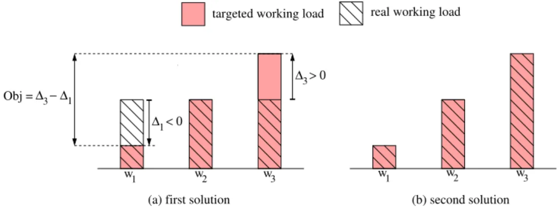
In a more formal way, the objective function we consider in this paper is the equity among workers, that we want to maximize. It is equivalent to minimize the inequity, defined as the difference between the highest and the lowest worker’s gap value, itself being the difference ∆i between the targeted workload and the real workload of the worker wi. We hence want to minimize ∆ = maxi∆i− mini∆i. A small difference between the highest gap and the smallest gap means that the workload is well balanced among workers. This objective criterion is illustrated on Figure1. In Figure1a, the difference between the targeted and the real workload is null for the worker w2, but not for w1 and w3, leading to a strictly positive value of the
objective function. On the contrary, on Figure 1b, the real workload perfectly matches with the targeted workload for each worker, and we hence have an optimal solution.
w1 w2 w3 w1 w2 w3 ∆ > 0 3 ∆ < 0 1 ∆ − ∆ 3 1
real working load targeted working load
(a) first solution (b) second solution Obj =
Figure 1: Objective function: equity
2.3. Feasibility
According to the global workload and the way it is spread along time-horizon, it may be impossible to find a solution that respects all the constraints. In particular, it may be difficult to cover every fixed tasks. If the decison-maker is not able to find an agreement with some employees in order to relax a few constraints (i.e. longer days or shorter breaks), then externals have to be hired to strenghten the regular workforce. In this case, the decision-maker tries to hire as few as possible externals, which requires a deep insight on the problem at hand to evaluate the different time-windows where additional workforce is needed on an acceptable timetable for regular workers, according to the structure of activity peaks, or unassigned tasks distribution. Therefore, in this paper (as in [10] and [14]), we relax the constraint which specifies that each task has to be assigned to exactly one employee. Hence, we can reach solutions with a partial assignment (i.e. some tasks are left unassigned). These solutions will be used by the decision-maker to evaluate externals requirements. However, a complete assignment is always better than a partial one. So, in this paper, we consider the minimization of the number of unassigned tasks and the minimization of the inequity among workers in a lexicographic order.
3. Constraints Modeling
This section is dedicated to the description of the Constraint Programming (CP) model introduced in [10] to handle the SDPTSP-E. The main idea of the model is to assign tasks to workers using a set variable model. More precisely, set variables T a[n] give the set of tasks assigned to worker n on the whole horizon, while set variables Da[d][n] give the set of tasks assigned to worker n on day d. The domain of these variables is initially defined according to employee skills and availabilities. While solving the problem, these sets are reduced by constraints filtering. Constraints over shift sequences are posted on boolean variables Sh[d][n], which define whether shift d is a working day or a day-off. Most of the legal constraints are posted on integer variables F i[d][n] and La[d][n], which stand for the starting and ending time of each day of each worker. These variables are linked with variables Da[d][n] so as to give the start (respectively the end) of the earliest (respectively latest) task assigned to a worker a day. The model also consider integer variables At[d][n], which define for each day and worker the minimal attendance time (i.e. the attendance time resulting from fixed tasks) and integer variables Ld[d][n] to tackle the duration of the lunch break. A matrix W d gives for each day and each worker the daily working time corresponding to the shift performed by the employee. In most cases, W d is equal to the length of the shift performed by the employee, however, if the employee has a lunch break, then W d is equal to the length of the shift minus the duration of the lunch break (one hour). Finally, the vector Bs gives for each worker the starting time of the weekly break.
Using those variables, it is possible to consider all the organizational and legal constraints within a CP approach as explained in [10].
The basic branching scheme considers the original variables T a[n], which corresponds pick an employee
n and assign him/her a task among the possible ones. The different variables ordering strategies either
consider first employee with a small amount of work (Less Working strategy) or employee with the highest amount of work (Most Working strategy). In the first case, the objective is to reduce unfairness of the partial solution, while in the second one the objective is to assign an amount of work to employees already involved. The principle here is to respect as much as possible the structure of the shifts currently in building and keep other employees free if possible. A parameter is fixed in order to have a limit on the amount of work that can be assigned to an employee. The interest here is to give priority to complete solutions.
Once a variable has been chosen, the Value Ordering strategy fixes the way to branch on the different possible values for this variable. Authors proposed different strategies based on biggest tasks or biggest overlap among tasks for example. the most interesting one here is the one named Lack of Nurse. This strategy leads to consider tasks that are difficult to cover, which means the number of eligible employees is the smallest.
The CP method leads in 5 minutes of computation to acceptable results regarding the number of unas-signed tasks and inequity, nevertheless in [14], it has been proven that it is possible to improve these results on several instances with a two-phase method. After investigation, it appears that the CP model is quite efficient to reach a solution, but is sometimes unable to improve it for a while, even if the solution is far away from the best one. On the opposite, the two-phase method is able to explore much more solutions, that may be quite far away from each other. For that reason, we decided to mix both advantages in a Large Neighborhood Search, based on the CP model.
4. Large Neighborhood Search
This section describes the Large Neighborhood Search (LNS) we propose to solve the SDPTSP-E. Note that LNS approaches have proven very efficient on many problems, such as Vehicule Routing Problems for example ([15]). Generally speaking, such an approach is a good way to improve the performance of exact approaches such as CP models, especially on large scale instances. Indeed, CP approaches are usually very good at finding a first solution, but they often encounter difficulties to improve them due to a lack of diversification during the search. On the contrary, LNS approaches enable to explore very different and interesting part of the search space. Therefore, using a CP model within an LNS framework allows to benefit from the filtering and propagation processes of CP, while exploring very different parts of the search space. Since the CP model is used only on a subpart of the whole problem, its ability to filter is much higher than
on the whole problem, leading to an efficient exploration. In the following, we first introduce the global structure of the LNS, before describing more precisely how we destroy and repair solutions.
4.1. Principles and global structure
Basically, LNS are based on an iterative process which successively destroy and repair a given solution so as to improve it step by step. The main idea is to focus on the part of the solution which looks suboptimal according to some heuristic indicators, so as to destroy it. This destruction leads to a partial solution, which maybe used as a starting point to reach a whole neighborhood of new solutions. The repair step consists in exploring a part of this neigborhood so as to find an improving solution. The improvment we are able to reach mainly depend on the subpart of the solution which is chosen to be destroyed. The most important thing is to destroy decision variables that are somehow related to each others, so as to be able to reach new solutions. To do so, a very effective way is to take into account the structure of the problem, so as to work on a sub-problem that is quite independent from the rest of the solution. Otherwise, one may have no choice but to rebuild the exact same solution, which is not desired. As a consequence, the destoyed part has to be large enough to allow the method to reach new solutions, and if possible to escape from a local optima, but not too large, in order to keep the reparation step efficient. Using a CP approach to repair the current solution enables to benefit from strong filtering, but this comes at computing price (compared to a simpler heuristic repair process). As a consequence, we choose to use the best solution at each iteration so as to avoid spending too much time in diversification (LNS already enables enough diversification). Indeed, we use two different and randomized operators to make the neighborhood varying at each step. The approach ends up when reaching a given time-limit.
In the context of a CP based LNS, the destroy step amounts to choosing a subset of the decision variables to uninstantiate, while other decision variables stay instantiated to their value in the best solution. As mentionned, a good way to design the destruction operators is to take into account the structure of the problem. In our context, we deal with both shifts design and tasks assignment, which naturally leads to consider two operators, one for each aspect. To handle the tasks assigment aspect, we use a time operator which unassigned a set of tasks that are fixed within the same time interval, so as to allow tasks exchanges between employees. To deal with the shifts design problem, we use an employee operator that unassigned all the tasks assigned to a subset of workers, so as to allow changes on their working shifts. One of those two different operators is randomly chosen at each iteration in order to destroy a part of the current solution. Then, this subpart of the solution is rebuilt with the CP approach, leading to a given neighbor.
4.2. Destruction operators
As mentionned previously, destroying a part of the current solution amounts to uninstantiating some decision variables. While doing this, it is important to keep the number of uninstantiated variables under control, so as to have an efficient repair step. We propose to use a parameter Size to fix the number of uninstantiated variables.
4.2.1. Time-oriented operator
This time-oriented destruction operator Topfocuses on the task assignment part of the SDPTSP-E. The
idea is to focus on a specific time-period so as to destroy the assignment of tasks that are overlapping in time (or close to each other). The time-interval is built randomly but in such a way that it covers a task that was left unassigned in the best solution. If every task is already assigned, one is picked randomly.
Once the task ti is chosen, a given number of tasks which are as close as possible to ti regarding their starting and ending times is picked. This number is given by the parameter Size, and discussed further. Note that the corresponding unassign time interval may not be centered around ti in order to allow this opertor reaching several neighborhoods even when picking the same initial task. All these considered tasks are unassigned, before using the CP model to rebuild a solution.
This operator enables a very high number of exchanges between employees who work on the selected time interval. Since tasks may last till 5 hours, it is important to consider a large time interval so as to give enough flexibility to the CP model in order to reach a better assignment between involved emmployees.
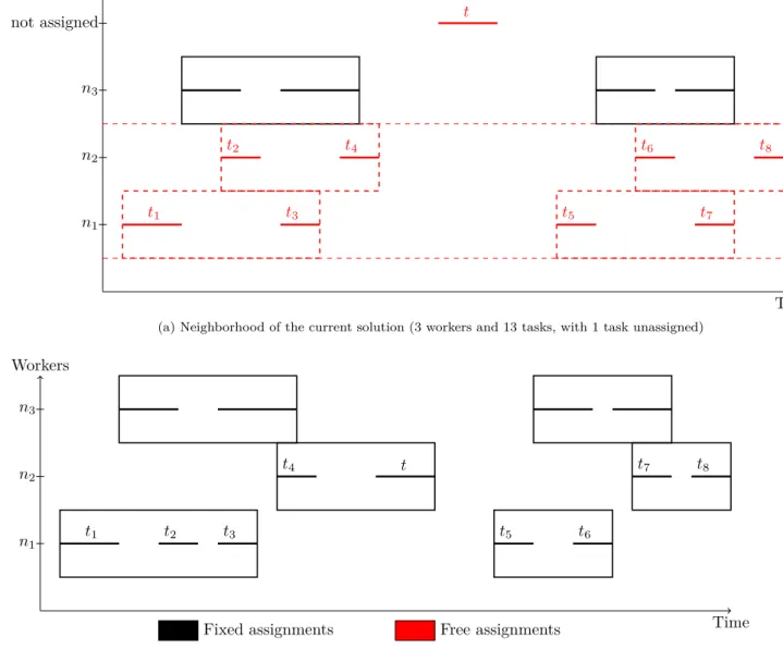
The use of this operator is illustrated on Figure2. On Figure (2a), we can see a part of a solution where task t is currently not assigned. Destroying the assignments of the three workers on that particular time interval allows to rebuild this part of the solutions in a better way, as we can see on Figure (2b), where every task is assigned. Note that, this improving solution may not be found by the CP model in case of a partial exploration of the neighborhood.
On the whole, the time-oriented operator is able to deeply impact a specific working day, but it may encounter big difficulties to change the sequence of working days. For instance, changing a day-off into a working day may be very difficult. Indeed, while trying to assign new tasks on an employee who was previously in a day-off, her/his other working days remain fixed, which would probably lead to violate some legal constraints. To that purpose, we propose next another operator that better fits the need of deep changes in the structure of an individual schedule.
4.2.2. Employee-oriented operator
In order to be able to perform deep changes in the structure of an individual schedule, we have to consider legal constraints that may block the shift assignment of an employee regarding the previous and followings shifts. To that purpose, we propose a second operator Pop that focuses on shifts design, and allows to
unassign the tasks of a subset of workers on the whole week. To limit the number of decision variables that are uninstantiated, we now use the parameter Size to control the number of employees whose schedule is destroyed.
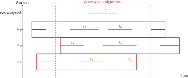
This operator randomly picks a subset of workers and destroy their whole schedule so as to be able to design new shifts sequences. This operator may be useful to build new shifts that cover some tasks. Figure
3 illustrates the interest of this operator. Figure (3a) shows a partial assignment, with an unassigned task lying in the middle of the resting time of all employees. As a consequence, this task cannot be assigned to any employees without changing at least two days (and probably the whole week). Using the employee-oriented operator enables to reach an interesting neighbor presented in Figure (3b), where new shifts have been created to cover task t.
4.3. Reparation step
After using one of the previously described operators, we use the CP model to explore the corresponding neighborhood by repairing the current partial solution. However, a complete exploration would presumably be too time-consuming, because of the size of the neighborhood which may be quite large. For that reason, and according to the fact that the CP model is better reaching a solution than improving it, we limit the search to the first solution reached at each iteration. Nevertheless, we add a new constraint to filter solutions that are strictly worse that the previous best one regarding the number of unassigned tasks. This configuration is quite unusual, because repairing the solution with the CP model takes more time than with a simple heuristic. Thus, one usually does not want to loose time exploring solutions that are not strictly better than the current one. However, it turns out this way of exploring the neighborhood is much more efficient in our context, as explained in the analysis of experimental results.
In order to repair the solution in an efficient way, one has to pay attention to the search strategy. In [10], the authors use several deterministic strategies, some of them being good at finding fair solutions, and others at assigning a maximum number of tasks. However, within a LNS framework, we assume that the same neighborhood (or nearly the same) may be explored several times, at different iterations. Therefore, using a deterministic strategy is presumably not a good idea, because it would lead to build the same solution many times. To deal with this issue, we propose to introduce some randomness in the search strategy while keeping the general idea of the best search strategies described in [10]. To that purpose, we introduced a new vector of integer variables emp[t], which gives the employee assigned to the task t. Obviously, we also post chanelling constraints between emp[t] and T a[n]. Then, it is possible to branch directly on emp[t], which makes it possible to benefit from some interesting search strategies of the literature.
To stay close to the strategy Lack of Nurse (LN), we could branch on the variable emp[t] with the smallest domain, but this strategy would also be determinitic. Therefore, we propose to branch on variables emp[t] according to a dom/wdeg strategy [2]. It means that we branch on the variable emp[t] with the smallest
destroyed assignments t3 t6 t1 t4 t2 t5 t Workers n1 n2 n3 not assigned Time (a) Neighborhood of the current solution (3 workers and 11 tasks, with 1 task unassigned)
t3 t5 t1 t t6 t2 t4 Workers n1 n2 n3 Time
Fixed assignements Free assignments
(b) Improved solution, all tasks are assigned
Destro y ed Assignmen ts t1 t3 t2 t4 t t5 t6 t7 t8 Workers n1 n2 n3 not assigned Time (a) Neighborhood of the current solution (3 workers and 13 tasks, with 1 task unassigned)
t1 t2 t3 t4 t t5 t6 t7 t8 Workers n1 n2 n3 Time
Fixed assignments Free assignments
(b) Improved solution, all tasks are assigned
ratio between its domain size and the number of backtracks due to a related constraint. Moreover, we use the last-conflict heuristic [11] on top of dom/wdeg, in order to give priority to the variable that has led to the last backtrack. Once the variable is chosen, we branch on the smallest possible value in its domain. This could be seen as a variant of the strategy Most Working (MW), because it leads to assign the workload in an unbalanced way (first workers are chosen in priority). On the whole, we obtain an adaptative search strategy that is close to the MW-LN strategy, which was one of the best strategy to build complete solutions.
4.4. Improvment step
Because of its structure, the proposed search strategy is presumably not very good at finding fair solu-tions, which is consistent with our goal to deal with the equity only in a second step, after finding a solution as complete as possible. Therefore, we need to deal with the equity in a post processing step. To do that, we use the local descent H∆introduced in [14]. Basically, it amounts to moving and swapping tasks between
workers so as to continuously improve the equity. Surprisingly, this descent is very efficient, even on solutions with a poor equity. Since the descent is quite fast, we decided to use it on each complete solution. In our case, it turned out to be very effective because, the LNS is able to generate a lot of different solutions, even for the same number of unassigned tasks.
5. Experimental results
The CP model has been implemented with Choco Solver, a Java Constraint Satisfaction Problem Solver [4]. However, while keeping the CP model proposed in [10], we updated its results because they were reached with the second version of Choco Solver, whereas the proposed LNS uses the third one. Instances have been run on an Intel Core i3-540 (3.06 GHz & 8G RAM) with a time limit of 5 minutes, which is the same configuration as in the CP approach of [10] and the two-phases method (M2P) of [14]. Note that instances have been introduced in [10], and can be found in [9]. We first present the results obtained with the LNS, then establish a comparison on all existing methods.
5.1. Large Neighborhood Search results
The results of the LNS are given in details in this section. We recall that a solution with a complete assignment of tasks to workers is referred to as a complete solution, by opposition to a partial solution. Within this section, we use the indicator «C» to indicate the number of complete solutions reached, «I» is the mean inequity value of the best solution in minutes (over complete solutions only), «A» is the average percentage of assigned tasks (over partial solutions only) and «T» is the mean computation time of best solutions, in seconds. Note that it is not possible to always find a complete solution in the instances of the benchmark. It has been proven that (at least) 102 instances do not admit a complete solution by an Integer Programming approach [8]. Hence, even if the benchmark is composed of 720 instances, we compare the number of complete solutions that we can reach with the 618 instances for which it may be possible to find a complete solution.
First of all, we focus on the parameter Size. Based on some preliminary computational tests, we decided to bound it depending on the size of the instance. Thus, when dealing with the employee-oriented destruction operator Pop, it ranges from 5 to 30 percents of the workers. Likewise, when dealing with the time-oriented
destruction operator Top, it ranges from 5 to 30 percents of the tasks. The parameter is initially set at its
lowest value, and increased after 50 iterations without improvements. To be able to escape local optima quickly, we do not simply increment the parameter Size, but we increase it by one quarter of its varying range (leading to increase Size by about 6 percents). To balance this quick and strong increase, the parameter
Size is decreased when an improving solution is found.
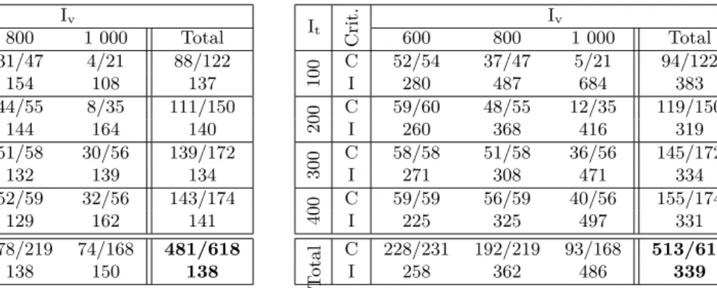
Before evaluating the interest of the LNS, which focus on improving an existing solution, we need to evaluate the peformance of the new branching strategy on variables emp[t]. To do that, we compare the initial solution of the CP model with the initial solution of the LNS (Tables1 and 2). Interestingly, the LNS branching strategy turned out to be more efficient than the best one of the CP model, over all possible branching strategies introduced in [10], which highlights the interest of the variables emp[t]. More precisely,
we can see that the LNS branching strategy leads to 513 complete solutions against 481 with the CP branching strategy, on a total of 618 instances where it is possible to have complete solutions. However, as expected, the inequity of those initial solutions is still very high.
It Crit. Iv 600 800 1 000 Total 100 C 53/54 31/47 4/21 88/122 I 129 154 108 137 200 C 59/60 44/55 8/35 111/150 I 133 144 164 140 300 C 58/58 51/58 30/56 139/172 I 132 132 139 134 400 C 59/59 52/59 32/56 143/174 I 141 129 162 141 T otal C 229/231 178/219 74/168 481/618 I 134 138 150 138
Table 1: Best initial solutions obtained with CP model and H∆ It Crit. Iv 600 800 1 000 Total 100 C 52/54 37/47 5/21 94/122 I 280 487 684 383 200 C 59/60 48/55 12/35 119/150 I 260 368 416 319 300 C 58/58 51/58 36/56 145/172 I 271 308 471 334 400 C 59/59 56/59 40/56 155/174 I 225 325 497 331 T otal C 228/231 192/219 93/168 513/618 I 258 362 486 339
Table 2: Initiales solutions with LNS (dom/Wdeg + last conflict-min value-H∆)
After those tests, we would like to introduce the results of the LNS with only one of the two destruction operators we proposed. We wanted to evaluate the impact of the two destruction operators.
First, we ran the LNS on all instances with only one destruction operator. Our goal was to determine wether or not these two operators are indeed complementary or not. As illustrated by Tables 3 and 4
it is clear that each operator leads to an improvment both on the number of complete solutions and the inequity. Therefore, we may conclude that these two operators allow to escape from local optima by reaching neighborhoods that are more difficult (if not impossible) to reach by the other one alone.
All those results include the improvment step H∆, used on all complete solutions. The local descent is
very effective, even when starting from poor solutions, and may lead to huge improvment on the inequity. Nevetheless, the resulting gap with the original equity of the considered solution is not possible to predict. Therefore, it is more effective to look for many different solutions, so as to call H∆as many times as possible.
It Crit. Iv 600 800 1 000 Total C 53/54 44/47 14/21 111/122 100 I 14 16 106 27 A 97,86 98,13 96,76 97,19 T 265 220 71 185 C 59/60 50/55 19/35 128/150 200 I 20 17 25 20 A 99,00 98,75 98,11 98,25 T 295 251 99 215 C 58/58 54/58 44/56 156/172 300 I 24 19 44 28 A 99,67 99,22 98,92 99,06 T 290 270 221 260 C 59/59 57/59 43/56 159/174 400 I 31 24 48 33 A 99,75 99,75 99,18 99,29 T 295 285 221 267 C 229/231 205/219 120/168 554/618 T otal AI 98,4623 98,6319 97,8550 98,0627 T 286 257 153 232
Table 3: LNS Results while using only Top(5 min)
It Crit. Iv 600 800 1 000 Total C 53/54 45/47 15/21 113/122 100 I 10 10 16 11 A 97,86 98,07 97,04 97,36 T 265 225 77 189 C 59/60 51/55 25/35 135/150 200 I 18 13 19 16 A 99,00 98,83 98,06 98,23 T 295 255 128 226 C 58/58 54/58 46/56 158/172 300 I 27 22 20 23 A 99,67 99,33 98,93 99,11 T 290 272 232 265 C 59/59 57/59 44/56 160/174 400 I 35 28 29 31 A 99,75 99,75 99,19 99,30 T 294 285 229 269 C 229/231 207/219 130/168 566/618 T otal AI 98,4623 98,6619 97,9222 98,1221 T 286 259 167 237
Table 4: LNS Results while using only Pop(5 min)
5.2. Overall comparison
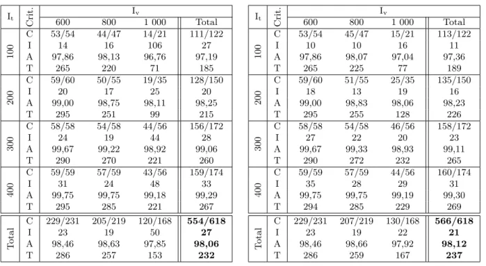
To evaluate the performance of the proposed LNS, we compare its results with those of the M2P, introduced in [14], because it is the best known method in the litterature. Tables 5 and 6 show that the LNS is able to find much more complete solutions than M2P and with a better equity. Moreover, partial solutions have on average a smaller number of unassigned tasks than with M2P. Note that the LNS is also slightly faster than the M2Pto reach its best solution.
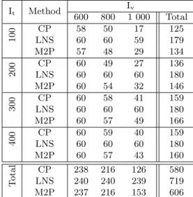
Even if the LNS gives very good results on average, we should also pay attention to its robustness regarding to the quality of its results. In this context, we would like to know if it gives very bad results on a few instances, so as to catch the configuration it fails to solve. We hence counted the number of best solutions computed by each method. On Table 7 the quality of a solution is evaluated in a classical way, whereas we just look at the number of unassigned tasks in Table8. Based on these results, it is clear that the LNS dominates the other aproaches, since it reaches 531 best solutions on a total of 720 instances, compared to around one hundred for the CP model and M2P. When considering only the number of unassigned tasks, the LNS performs even better, since it finds the best solution 719 times out of 720.
It Crit. Iv 600 800 1 000 Total C 54/54 46/47 20/21 120/122 100 I 17 14 17 16 A 97,67 98,07 97,10 97,38 T 144 117 128 127 C 59/60 53/55 29/35 141/150 200 I 27 24 26 26 A 99,00 98,71 98,90 98,13 T 73 175 162 162 C 58/58 54/58 47/56 159/172 300 I 33 26 29 29 A 99,67 99,33 98,90 99,10 T 180 170 171 172 C 59/59 58/59 44/56 161/174 400 I 34 31 38 34 A 99,75 99,75 99,27 99,34 T 278 289 195 209 C 230/231 211/219 139/168 581/618 T otal AI 98,4128 98,6024 97,9530 98,1227 T 158 154 155 155
Table 5: LNS Results in 5 minutes
It Crit. Iv 600 800 1 000 Total C 53/54 42/47 11/21 106/122 100 I 28 35 72 35 A 97,50 97,78 96,71 97,05 T 145 155 167 156 C 59/60 50/55 22/35 131/150 200 I 34 35 42 36 A 99,00 98,60 97,72 97,93 T 166 138 156 154 C 58/58 53/58 42/56 153/172 300 I 40 38 46 41 A 99,67 99,19 98,76 98,94 T 191 186 174 184 C 59/59 55/59 40/56 154/174 400 I 47 44 51 47 A 99,75 99,70 99,01 99,17 T 236 202 196 211 C 229/231 200/219 115/168 544/618 T otal AI 98,2838 98,4738 97,6849 97,9040 T 184 170 173 176
Table 6: M2P results in 5 min
It Method Iv 600 800 1 000 Total 100 CP 2 3 5 LNS 56 54 41 151 M2P 4 4 16 24 200 CP 7 4 11 LNS 47 52 50 149 M2P 9 9 7 25 300 CP 28 6 3 37 LNS 26 50 46 122 M2P 8 5 11 24 400 CP 40 9 6 55 LNS 20 42 47 109 M2P 1 13 9 23 T otal LNSCP 14975 19817 18416 108531 M2P 22 31 43 96
Table 7: Number of best overall results
It Method Iv 600 800 1 000 Total 100 CP 58 50 17 125 LNS 60 60 59 179 M2P 57 48 29 134 200 CP 60 49 27 136 LNS 60 60 60 180 M2P 60 54 32 146 300 CP 60 58 41 159 LNS 60 60 60 180 M2P 60 57 49 166 400 CP 60 59 40 159 LNS 60 60 60 180 M2P 60 57 43 160 T otal LNSCP 238240 216240 126239 580719 M2P 237 216 153 606
Table 8: Number of best results on the number of unassigned tasks
6. Concluding remarks
This paper deals with a new method for the Shift-Design Personnel Task Scheduling Problem with Equity. This real-life problem deals simultaneously with the assignment of fixed tasks and the design of personnel shifts, so as to minimize the number of unassigned tasks while sharing the workload between employees in a fair way.
We presented here a Large Neighborhood Search, based on a CP model and a local descent. This method clearly improves the state-of-the-art results and it gives new best solutions on several instances. The research
avenues that still stand for this problem now deal with two main points. On one hand, it would be useful to improve the quality of lower bounds so as to evaluate more precisely the quality our approach. On the other hand, it would be interesting to try an approach based on a column generation model, because it has proven very efficient on personnel scheduling, and the structure of the problem is suitable for this kind of method.
[1] Alfares, H.K.: Survey, Categorization, and Comparison of Recent Tour Scheduling Literature. Annals of Operations Research 127, 145–175 (2004)
[2] Boussemart, F., Hemery, F., Lecoutre, C., Sais, L.: Boosting systematic search by weighting constraints. In: 16th European Conference on Artificial Intelligence. vol. 16, p. 146 (2004)
[3] Burke, E.K., De Causmaecker, P., Berghe, G.V., Landeghem, H.V.: The state of the art of nurse rostering. Journal of Scheduling 7, 441–499 (2004)
[4] CHOCO Team: choco: an Open Source Java Constraint Programming Library. Tech. rep., Ecole des Mines de Nantes (2010)
[5] Ernst, A.T., Jiang, H., Krishnamoorthy, M., Sier, D.: Staff scheduling and rostering: A review of applications, methods and models. European Journal of Operational Research 153(1), 3–27 (2004)
[6] Kolen, A.W.J., Lenstra, J.K., Papadimitriou, C.H., Spieksma, F.C.R.: Interval Scheduling: A Survey. Naval Research Logistics 54, 530–543 (2007)
[7] Krishnamoorthy, M., Ernst, A.T.: The personnel task scheduling problem. In: Optimization Methods and Applications, pp. 343–367 (2001)
[8] Lapègue, T., Bellenguez-Morineau, O., Prot, D.: Ordonnancement de personnel avec affectation de tâches: un modèle mathématique. In: Roadef’13 (2013)
[9] Lapègue, T., Fages, J.G., Prot, D., Bellenguez-Morineau, O.: Personnel Task Scheduling Problem Library (2013),https: //sites.google.com/site/ptsplib/smptsp/home
[10] Lapègue, T., Prot, D., Bellenguez-Morineau, O.: A constraint-based approach for the Shift Design Personnel Task Schedul-ing Problem with Equity. Computers and Operations Research 10(40), 2450–2465 (2013)
[11] Lecoutre, C., Sais, L., Tabary, S., Vidal, V.: Reasoning from last conflict(s) in constraint programming. Artificial Intelli-gence 173(18), 1592–1614 (2009)
[12] Mabert, V.A., Watts, C.A.: A Simulation Analysis of Tour-Shift Construction Procedures. Management Science 28(5), 520–532 (1982)
[13] Pisinger, D., Ropke, S.: Large neighborhood search. In: Gendreau, M., Potvin, J.Y. (eds.) Handbook of Metaheuristics. Forthcoming, 2nd edn. (2009)
[14] Prot, D., Lapègue, T., Bellenguez-Morineau, O.: A two-phase method for the Shift Design and Personnel Task Scheduling Problem with Equity objective. International Journal of Production Research 53, 7286–7298 (2015)
[15] Shaw, P.: Using Constraint Programming and Local Search Methods to Solve Vehicle Routing Problems. In: Principles and Practice of Constraint Programming (CP 1998), volume 1520 of LNCS. pp. 417–431 (1998)