UNIVERSITÉ DU QUÉBEC À MONTRÉAL
EFFET DE L'ASSOMBRISSEMENT PLANÉTAIRE SUR
LA
CROISSANCE DES
ARBRES
THÈSE
PRÉSENTÉE
COMME EXIGENCE PARTIELLE
DU DOCTORAT EN BIOLOGIE
PAR
LIONEL HUMBERT
Avertissement
La diffusion de cette thèse se fait dans le rèspect des droits de son auteur, qui a signé le formulaire Autorisation de reproduire et de diffuser un travail de recherche de cycles supérieurs (SDU-522 - Rév.01-2006). Cette autorisation stipule que «conformément à l'article 11 du Règlement no 8 des études de cycles supérieurs, [l'auteur] concède à l'Université du Québec à Montréal une licence non exclusive d'utilisation et de publication de la totalité ou d'une partie importante de [son] travail de recherche pour des fins pédagogiques et non commerciales. Plus précisément, [l'auteur] autorise l'Université du Québec à Montréal à reproduire, diffuser, prêter, distribuer ou vendre des copies de [son] travail de recherche à des fins non commerciales sur quelque support que ce soit, y compris l'Internet. Cette licence et cette autorisation n'entraînent pas une renonciation de [la] part [de l'auteur] à [ses] droits moraux ni
à
[ses] droits de propriété intellectuelle. Sauf entente contraire, [l'auteur] conserve la liberté de diffuser et de commercialiser ou non ce travail dont [il] possède un exemplaire.»REMERCIEMENTS
Je tiens à remercier en premier lieu Frank Berninger d'avoir accepté œêtre le
directeur de cette thèse et de m'avoir laissé autant de libertés. Mes remerciements
vont conjointement et tout particulièrement à Fernando Valladares et Dan Kneeshaw
pour leur soutien et leur enthousiasme qui m'ont permis de mener à bien ce projet.
Je voudrais également remercier Christian Messier, notre cher ex-Directeur du C.E.F.
pour son écoute et son soutien lors des étapes cruciales de cette thèse. J'aimerais aussi
le remercier pour son investissement dans cette magnifique structure qu'est le C.E.F.,
sans qui les travau .. '< présentés ici n'auraient probablement pu aboutir . .Je tiens donc
à remercier Luc Lauzon, Danielle Charon, Daniel Lessieur et Melanie Desrocher pour
lem accueil au sein du centre, ainsi qu'Alain Leduc l'autre adorateur du saint nectm- de
9h et Herve Bescond pour nos rechutes de 13h. Merci à Paul Sheppm·d de l'Université
d'Arizona pour m'avoir accueilli à Tucson et permis d'écrire les dernières lignes de cette
thèse sous une chaleur accablante tout en me faisant économiser des tonnes de
co2
etprivant ainsi les Mesquites, Palo verdes et Saguaros d'un peu de leurs nutriments. Je
tiens particulièrement à remercier Henrik et sa famille, ainsi que Dominique et Geneviève
pour nos discussions autour decliner et petits plaisirs brassés. Et un grand merci à Gab,
Claudia, Florent, Matt, Dominic Seneca.l, Caroline, Leila, Sophie, Marie-Claude, Adi,
Astrid, Philippe Tremblay, Karine et Karine et Karine (elles se reconnaîtront), Eric,
Yassin, Frank et tous mes amis pour lem soutien.
Merci enfin à mes pru:·ents, grands parents, à ma petite sœur Emeline et ma chère
et tendre qui m'ont perrrùs d'être comme en France à chacune de leurs visites et de grosses bises à ma petite filleule Ninon, à mon petit filleul Noé, à leurs parents et à toute ma famille.
"En terme de préhistoire, on parle de l'âge de pierre, de l'âge du fer, de l'âge du bronze. En survolant toute l'histoire de l'humanité, ne devrait-on pas parler de l'âge du bois, du charbon, du pétrole ou de l'atome?"
Roger Molinier, 1991 tiré de L'Écologie à la croisée des chemins
LISTE DES FIGURES . LISTE DES TABLEAUX RÉSUMÉ . . . INTRODUCTION
TABLE DES MATIÈRES
Xl xv XVll 1
NOTE SUR LES CHAPITRES . 15
CHAPITRE I
USE OF INDEPENDENT COMPONENT ANALYSIS WITH TREE RING WIDTH
SERIES . . . . . . . . 17
1.1 INTRODUCTION 17
1.2 DEFINITION . . . 19
1.3 SIMULATED DATA AND ANALYSIS. 20
1.4 RESULTS AND DISCUSSION . . . . . 24
1.4.1 TI·end Recovering within Data Set 1 24
1.4.2 Detection of Spikes and Recovery of Their Values within Data Set 2 and 3 . . . . . . . . . . . . . . 25 1.4.3 Complex Series Analysis of the Data Set 4 28 1.5 CONCLUSION . . . . . . . . . . . . . . . . . . 32 CHAPITRE II
IDENTIFYING INSECT OUTBREAKS: A COMPARISON OF A BLIND-SOURCE
SEPARATION METHOD WITH HOST VS NON-HOST ANALYSES 37
2.1 2.2
2.3
INTRODUCTION . . MATERIALS AND METHODS 2.2.1 Data and Insect Information 2.2.2 Analyses .. RESULTS. . . . ... . .. 38 40 40 43 45
2.3.1 Analysis of Ponderosa Pine as a Host Species of Pandora Moth . 46
2.3.2 Analysis of Ponderosa Pine as a Non-host Species for Western Spruce Budworm and Thssock Moths . . . . . . . . . . . . . . . . 46
2.4.1 Growth Changes 55
2.5 CONCLUSION . . . 56
CHAPITRE III
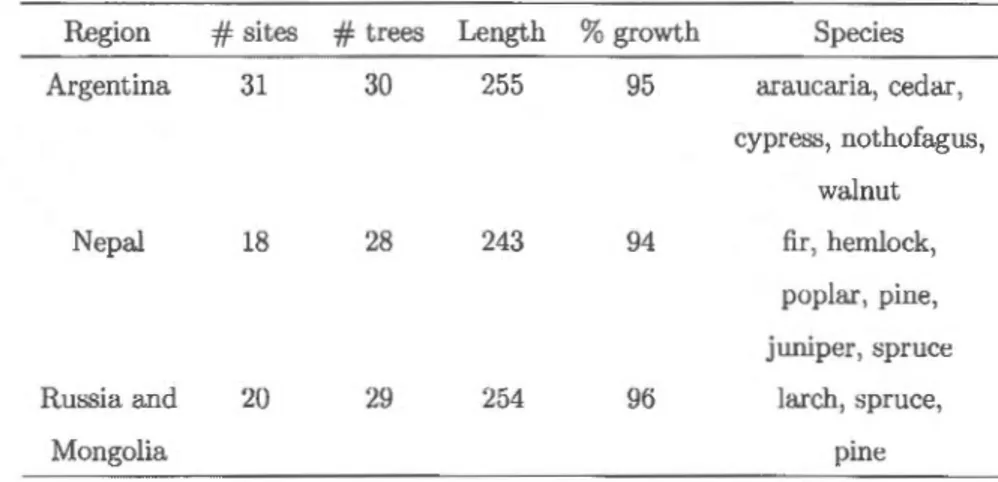
TREE GROWTH, SOLAR FORCING AND C02 FERTILIZATION ACROSS HIGH ALTITUDE AND HIGH LATITUDE FORESTS IN ARGENTIN A, NEP AL
AND RUSSIA . . . . . . . . 59
3.1 INTRODUCTION 60
3.2 DATA . . . 62
3.3 METHODS 64
3.4 RESULTS . . 67
3.4.1 Independent Component Analysis 3.4.2 Running correlations .
3.5 DISCUSSION . . .
3.5.1 Independent Component Analysis
3.5.2 Granger Causality and Running Correlation Robustness .
3.5.3 Regional Estimate and Pollution Effect . . . .. .
3.5.4 Light and Temperature Limitation in Northern Forest CHAPITRE IV
THE INFLUENCE OF ATMOSPHERIC TRANSPARENCY ON TREE GROWTH 67 67 74 74 75 76 77
VARIES ACROSS ECOSYSTEMS 83
4.1 INTRODUCTION . . . 84
4.2 MATERIAL AND METHODS 86
4.2.1 Data . . . . 4.2.2 Data Analysis. 86 89 4.3 RESULTS . . . 90 4.4 DISCUSSION . 95 CHAPITRE V
TREE GROWTH FOLLOWING PINATUBO AND EL CHICHON ERUPTION :
A GLOBAL ANALYSIS 101
5.1 INTRODUCTION . . . 102
lX
5.2.1 Data . . . . . . . . . . . . . . . . . . . . . . . . . . . . . . . . 104
5.2.2 Ttee Ring Width Analysis . . . . . . . . . . . . . . . . . . . . 104
5.2.3 Statistics . . . . . . . . . . . . . . . . . . . . . . . . . . . 106
5.3 RESULTS . . . . . . . . . . . . . . . . . . . . . . . . . . . . . . 107
5.3.1 Detection . . . . . . . . . . . . . . . . . . . . 107
5.3.2 Volcanoes . . . . . . . . . . . . . . . . 107
5.3.3 Multivariate Analysis . . . . . . . . . . . . . . . . 108
5.3.4 Latitude and Elevation Effect . . . . . . . . . . . . . . . . 113
5.4 DISCUSSION . . . . . . . . . . . . . . . . . . . . . . . . . . . . . . . . . 117
CONCLUSION . . . . . . . . . . . . . . 119
APPENDICE A CHAPTER II : ICA SENSITIVITY . . . . . . . . . . . . . . . . . . . . 123
APPENDICE B CHAPTER III : MAPS WITH SITE LOCATIONS . . . . . . . . . . . 127
APPENDICE C CHAPTER III : SPECTRUM ANALYSIS OF SIBERIA'S TEMPERATURE AND PRECIPITATION DATA . . . . . . . . . . . . . . . . . . 131
APPENDICE D CHAPTER III : RESULT OF ENGEL-GRANGER COINTEGRATION TEST 133 APPENDICE E CHAPTER IV: TREE RING WIDTH SERIES AVAILABLE FOR EACH YEAR 143 APPENDICE F CI-IAPTER IV: DATA SUMMARY . . . .. . . .. . . . 145
APPENDICE G CHAPTER IV: AVERAGING OF ANOMALIES AND CHANGE OF THE DOWNWELLING SHORTWAVE RADIATION AT SURFACE FROM 9 MOD-ELS . . . . . . . . . . . . . . . . . . . . . . . . . . 159
APPENDICE I-I CHAPTER V : SPECIES GROWTH RESPONSE FOLLOWING EL CHICHON AND MOUNT PINATUBO VOLCANIC EVENTS (FULL TABLE) . . . 161
APPENDICE I CHAPTER V : EFFECT OF LATITUDE AND ELEVATION ON TREE R.E-SPONSE FOLLOWING EL CHICHON AND MOUNT PINATUBO VOLCANIC EVENTS . . . 169
LISTE DES FIGURES
Figure Page
0.1 Concentration atmosphérique des gaz à efl:'et de serre de longue durée de vie au cours des derniers 2000 ans . . . . . . . . . . . . . . . . . 2
0.2 La photosynthèse . . . .. . . . 3
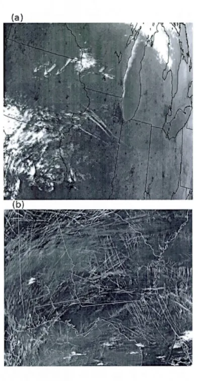
0.3 Images de Radiomètre Avancé à TI:ès Haute Résolution infrarouges mon -trant les traînées de condensation générées par les avions . . . . . . . 5
0.4 Vue du Half-Dome depuis Cloud Rest au parc national de Yosemite. 6
0.5 Flux radiatifs de surface dus aux forçages naturels ainsi qu'anthropiques entre les années 1860 et 2000 . . . . . . . . . . . . . . . . . . . 7
0.6 Radiations solaires à ondes courtes arrivant au niveau du sol 8
O. 7 Comportement de la lumière dans la canopée . . . . . 9
1.1 Example of constructed series with the components used to build it . 22
1.2 Analysis of complex series schematic representation . . .
1.3 Results of the recovered trends and disturbance pattern
23
26
1.4 Recovering of one spike with increasing number of series without spike 30
1.5 Spikes recovering from independent cornponent analysis . . . . . . 31
1.6 Resulting trend and cycle of independent components extractecl cluring the analysis of complex simulated data . . . . . . . . . . . . . . . . . . . 32
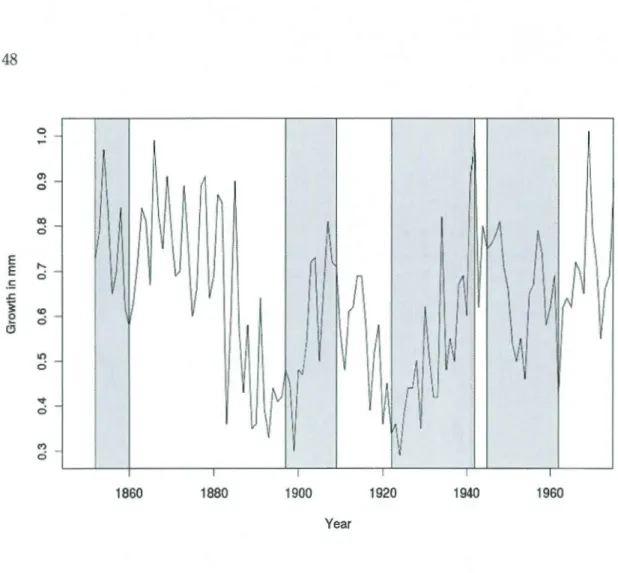
2.2 Growth of a single non-host tree fi:·om Swetnam et al. (1995), site number or032 . . . . . . . . . . . . . . . . . . . . . . . . . . . . . 48
3.1 Autocorrelation function, spectrum analysis and solar cycle correlation with growth of an extracted environmental component from a Russian site 68
3.2 Soh:u· cycle correlation with noisy and noiseless tree growth data . . . . 69
3.3 Correletion of temperature, precipitation and solar cycle with tree growth fi:·om 1750 to 2000 in Nepal, Argentina and Siberia . . . . . . . . 71
3.4 Volcanic events affecting the correlation between solar cycle and gTowth in Nepal . . . . . . . . . . . . . . . . . . . . . . . 73
4.1 Map with the aerosol optical depth site locations highlighted in red . 88
4.2 Distribution of the values for aerosol optical depth . . . . . . . . . 92
4.3 Relationship between the atmospheric transparency and the correlation between solar cycle and growth during the 1933-1954 period . . . . . . 93
4.4 Frequency distribution of the correlation values between solar cycle and growth for the different ecosystems covered in this study . . . . . . . 94
4.5 Long-term change of the relationship between atrnospheric transparency and the solar cycle/tree growth correlation . . . . . . . 96
5.1 Distribution of data with regard to their distance to the volcano . . . . 105
5.2 Example of volcanic distmbance affecting tree growth extracted by ICA in Arizona site number 558 . . . . . . . . . . . . . . . . . . . . . . . . . 107
Xlii
5.4 Species scores and biplot arrows representation for the redundancy anal -ysis of tree growth response to volcanic events . . . . . . . . . . 114
5.5 Effect of latitude on tree response at high elevation with cmve of signifi-cant relationship . . . .
A.1 Results of spike detection by ICA .
B.1 Argentina tree ring width site locations map .
B.2 Nepal tree ring width site locations map .
B.3 Russia tree ring width site locations map
116
124
128
129
130
C.1 Spectrum analysis of Siberia's temperature and precipitation data 132
E.1 Number of tree ring width sites (TRW, for a total of 841) with data for each year over the 1700-2005 period. . . . . . . . . . . . . . 144
G .1 Anomalies and change of the downwelling shortwave radiation at surface from 9 models . . . . . . . . . . . . . . . . . . . . . . 160
1.1 Effect of latitude and elevation on tree response for Rpart groups 170
1.2 Effect of latitude and elevation on tree response for RDA groups 171
LISTE DES TABLEAUX
Tableau Page
1.1 Performance of the independent component a.nalysis compared to a mean series for trends and disturbance pattern recovering . . . . . . . . . . 27
1.2 Results of the detection of spikes in a set of series without spikes by the independent component analysis . . . . . . .
2.1 Surnmary of data uscd in analyses of Chapter II
2.2 Results from the re-analysis of non-host species data of Ryerson, Swetnam 29
41
& Lynch (2003) . . . . . . . . . . . . . . . . . . . . . . . . . . . . . 49
2.3 Results from the re-analysis of non-host species data of Swetnam et al. (1995) . . . .
3.1 T'tee ring width data smmnary
3.2 Cointegration test and Granger causation results between tree growth 50
64
and the solar cycle, temperature and precipitation . . . . . . . . . 70
3.3 Student's t-test results concerning the slope of the correlation between the independent component of interest and environmental variables . 7 4
3.4 Aerosol optical depth daily average for various location worldwide . 78
4.1 Evolution of the relationship between Aerosol Optical Depth and the correlation between Solar lrradiance and Growth . . . . . . . . . . . . . 95
5.1 Descriptive values for tree growth response following the volcanic eruption of El Chich6n and the Pinatubo . . . . . . . . . . . . . . . 108
Pinatubo volcarùc events . . . . . . . . . . . 112
5.3 Comparison of Regression Tree and Redundancy Analysis groups 115
A.1
D.1
Chapter II Spike detection results by ICA . . . .. . .
Chapter III Results for Engel-Granger cointegration test
125
134
D.2 Chapter III Results for Engel-Granger cointegration test ( continued) . 139
F.1 Chapter IV Data summary . . . . . . . . . . . . . . . . 146
H.1 Chapter V Species growth response following El Chich6n volcanic event 162
H.2 Chapter V Species growth response following Mount Pinatubo volcanic event . . . . . . . . . . . . . . . . . . . . . 165
RÉSUMÉ
L'utilisation des combustibles fossiles, en plus d'augmenter la concentration du
C02 mondial, abaisse la lumière directe que l'on reçoit du soleil en la di th-actant. Cet
"as-sombrissement global" peut, contrairement au
co
2
'
diminuer la croissance des arbres caril diminue la lumière donc la photosynthèse est moins importante. L' "assombrissement
global", dans le cadre de l'analyse de cernes, présente un atout pa.r rapport à évaluer
seulement l'effet du C02 comme changement global. On peut théoriquement déduire son
effet sur les cernes en observant l'évolution de la relation entre les cernes et la lumière.
Cela est possible car la lumière arrivant à la surface du globe suit un cycle déternùné de 11 ans. Ce cycle, le cycle solaire, est bien connu et nous savons qu'il exerce un ef-fet sur les cernes depuis les travaux de Douglass au début du siècle passé. L'étude de l'effet de l' "assombrissement global" sur les cernes est donc un sujet de choix si l'on
veut examiner une variable qui peut induire un changement lent sur le long terme, ou
une tendance. Mais les méthodes traditionnelles d'analyse des cernes de croissance sont
mal adaptées à la recherche de telles tendances. Au cours de cette thèse nous avons
testé des méthodes statistiques modernes pour l'analyse de l'effet de la lurrùère en lien
avec l' "assombrissement global" sur les cernes de croissance des arbres. Ces méthodes
ont ensuite été utilisées pour détecter les tendances environnementales dans les cernes. Ainsi, l'utilisation d'une méthode aveugle de séparation des signaux sources, l'analyse
en composants indépendants (ICA), évite certaines suppositions et permet d'éliminer
les effets des perturbations sur la croissance.
Le premier chapitre de cette thèse décrit en détail cette méthode et la teste sur
des données simulées de cernes de croissance d'arbres. On retrouve donc la composante
climatique de la croissance isolée, telle que décrite dans le mode! linéaire agrégé classique.
Le second chapitre applique cette méthode différemment. En effet, nous avons
voulu tester la capacité de l'ICA à trouver des perturbations. On a donc ré-analysé des
données dendroécologiques provenant de publications traitant d'épidemies d'insectes.
Nos résultats montrent que l'ICA est capable de detecter les perturbations dans les
cernes de croissance déjà identifiées et que cette méthode peut permettre l'analyse des
perturbations lorsqu'il est difficile de mettre en œuvTe les méthodes traditionnelles avec
climatiques pour voir si la température, les précipitations et la lumière ont un effet sur les cernes. Nos résultats montrent que la corrélation entre la lumière et les cernes augmente progressivement au cours du temps. Cette augmentation semble être en relation avec le niveau de pollution atmosphérique. Elle est plus forte au Népal où la proximité de l'Inde apporte de nombreux polluants, un peu moins forte en Argentine et non présente en Sibérie où la pollution est majoritairement hivernale (donc durant la saison sans croissance arborescente). Le niveau de pollution semble donc influencer la relation entre les cernes et la lumière. On peut ainsi supposer que la lumière diffuse produite par la pollution influence positivement la croissance, en contraste avec notre supposition originale.
Au chapitre IV, nous voulions vérifier si le niveau de pollution influençait effective-ment l'effet de la lumière sur la croissance des arbres au niveau mondial. Nous avons comparé les données d'un réseau mondial de 183 stations de mesures de la pollution atmosphérique avec l'effet du cycle solaire sur les cernes de 841 sites forestiers à prox-imité de ces stations. Les résultats montrent que pour les sites forestiers provenant des écosystèmes méditérranéens et altitudinaux la pollution augmente l'effet de la lumière diffuse sur la croissance depuis 1960.
Dans le chapitre V j'utilise la réaction des arbres lors des deux plus importantes éruptions volcaniques du siècle dernier pour voir si la lumière diffuse augmente bien la croissance des ru·bres et que cet effet n'est pas du à la baisse concomitante de la température. Ces deux éruptions sont d'intensité égale, mais au cours de l'une d'elles un événement climatique (El Niiio) a masqué son effet de refroidissement. L'analyse de 210 sites forestiers sélectionnés de façon aléatoire dans le monde entier, nous indique que c'est bien la lumière diffuse qui infiuence la croissance et non pas la baisse de température qui lui est associée.
Au cours de cette thèse nous avons montré que la lumière modifiée par 1' "assom-brissement global", c'est-à-dire une baisse de la lumière directe au profit de la lumière diffuse, augmente la croissance des arbres. Ce phénomène est surtout présent pour les écosystèmes qui sont lirnités en eau. Cet effet de la lurnière diffuse pourrait rendre difficile l'identification d'un effet de la fertilisation due au C02 .
INTRODUCTION
Depuis la conférence de Rio en 1992, puis celle de Kyoto en 1997 (Houghton, Callander et Varney, 1992; United Nations, 1997), l'accent a été mis sur la réduction de1:> émission1:> de gaz à effet de serre. Cet effet de serre est naturellement lié à la présence de vapeur d'eau pour 75% et de certains gaz. Or, la concentration atmosphérique du dioxyde de carbone (C02) et du méthane (CH4) a été fortement influencée par les activité1:> humaines (Figure 0.1 tirée de Salomon et al., 2007). Les émissions de C02 sont le résultat direct de l'utilisation de combustibles fossiles comme source d'énergie. Mais en plus de libérer du co2, leur combustion produit un grand nombre de particules qui changent d'autres caractéristiques de l'atmosphère. Notamment, les propriétés optiques de l'atmosphère sont affectées par les particules en suspension qui vont diffracter, absorber et réfiechir la lumière.
Les arbres, par une réaction physico-chimique, la photosynthèse (Figure 0.2), vont subir ces changements et utiliser des éléments qui sont dans l'atmosphère et/ou qui peuvent y être modifiés. La modification de la composition et du comportement de l'atmosphère, vont de plus participer à son réchauffement, au refroidissement de surface et à la form a-tion des nuages. Sachant que les principaux éléments de cette réaction physico-chimique sont : le co2, la lumière, l'eau et que tout dépend de la température ambiante, il est probable que la croissance des arbres soit affectée par l'utilisation des combustibles fossiles.
Il est connu depuis les années 1920/1930 qu'une augmentation de la concentration at-mosphérique du C02 stimulait la croissance des plantes (Hoover, Johnston et Brackett, 1933; Thomas et Hill, 1949), mais l'effet de l'augmentation du C02 sur la croissance des arbres est depuis sujet à controverse. LaMarche et al. (1984) ont conclu que l'augmen -tation de la croissance des arbres dans les années 80 était plus élevée que celle estimée
r
2
Concentrations of Greenhouse Goses from 0 to 2005
400 2000 1800 - Corbon Dioxode (C02 ) ,...--... .D - Methane (CH.) 1600 0... 350 0... '-"' - Nitrous Oxide (N20) 0 "' z 1400 -:g: 0... ,...--... E 0... 0... 1200
t
'-"'0
300 u 1000 800 250~~~~~~~~~~~~~~~~~~~~~600 0 500 1 000 1 500 2000 Y eorFigure 0.1 Concentration atmosphérique des gaz à effet de serre de longue durée de vie
au cours des derniers 2000 ans. Les unités de concentration sont en parties par million
3. Carbon dloxlde enters leat through sl:omala
Figure 0.2 La photosynthèse, @Discover Science, Scott, Foresman & Co. 1993 3
par les hausses de température, ce qui serait du à une fertilisation au C02. Toutefois, Graumlich (1991) et, plus récemment, Jacoby et D'Arrigo (1997) concluent que le::; in-dices permettant d'observer un effet de fertilisation au CO en conditions naturelles dans les cernes semblent être très limités. Mais le problème principal reste que le CO et les autres éléments influencés par les changements globaux évoluent lentement d'une année à l'autre. Il y a donc une faible tendance à long terme qui s'est installée. Graumlich (1991) et Jacoby et D'Arrigo (1997) soulignent d'ailleurs qu'avec les méthodes d'analy-ses utilisées, les tendances comme celle du co2 sont difficiles à capter car la croissance des arbres est sujet à d'autres phénomènes climatiques. De nouvelles méthodes d'anal-yse devraient donc être nécessaires. L'augmentation de la lumière diffuse, l'absorption de la lumière du soleil par des particules aérosol (Hansen et al., 2000; Ramanathan et al., 2001) et les traînées de condensation des avions (Murcray, 1970; Penner et al., 1999; TI:avis, Carleton et Lauritsen, 2004) pourraient également avoir un effet direct ou indirect sur la croissance des arbres et le bilan de carbone. Le phénomène le plus
visuel est certainement celui des traînées de condensation formées par les avions qui sont constituées de particules de glace. Cette formation de glace est principalement due au réchauffement de l'air et à sa condensation en sortie des réacteurs (Schumann, 2005).
Le phénomène est accentué par les impuretés de l'air et la combustion incomplète du kérosène (Schumann, 2005) et peut former des traînées persistantes alors qu'elles dis-paraissent rapidement en temps normal. Habituellement ces traînées sont présentes en
grand nombre (Figure 0.3 b) et leur impact climatique n'était que spéculatif avant la tragédie du 11 septembre 2009. Après cette tragédie, l'espace aérien américain fut inter-dit (Figure 0.3 a) et, le lendemain, des observations au sol ont montré une augmentation de la différence de température entre le jour et la nuit de 1C (Travis, Carleton et L au-ritsen, 2002). Malgré des critiques (Kalkstein et Balling, 2004; Solomon et al., 2007),
cet impact climatique des traînées d'avions semble réel (Travis, Carleton et Lauritsen, 2004) avec une augmentation de l'ordre de 0.2-0.3°C tous les dix ans (Minnis et al., 2004; Stordal et al., 2005; Zerefos et al., 2003) même si beaucoup d'incertitudes subsis-tent (Burkhardt et al., 2008). De plus elles favorisent la formation de cirrus (Mannstein
et Schumann, 2005) qui rendent la lumière plus diffuse et contribuent au réchauffement global (Marquart et al., 2005; Fichter et al., 2005).
Comme les cirrus, tous les nuages vont diffracter et absorber la lumière. Mais la diffrac -tion et l'absorption de la lumière peuvent également avoir d'autres origines. L'utilisation de combustibles fossiles émet énormément de particules fines et de particles qui forment des aérosols comme les substances organiques volatiles ou le S02 (Figure 0.4). C'est
également le cas de phénomènes naturels comme les feux de forêts ou les éruptions
volcaniques.
Ces particules produisent une baisse des radiations directes et augmentent les radiations
diffuses (Dutton et Bodhaine, 2001; Robock, 2000, 2005). Ce phénomène agit au niveau
de la planète entière (Figure 0.5) et il a été qualifié d'"assombrissement global" (Stanhill et Cohen, 2001; Ramanathan et al., 2001). La transparence de l'atmosphère a d'ailleurs
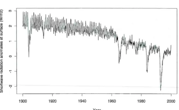
diminué graduellement depuis 1850 (Figure 0.6 adaptée de Romanou et al., 2007). Ces
5
Figure 0.3 Images de Radiomètre Avancé à Très Hante Résolution (AVHRR) in-frarouges montrant les traînées de condensation générées par les avions (Photos de la NASA, libre de droits). L'image (a) montre l'avion présidentiel et son escorte le 12 septembre 2001 alors que l'espace aérien était interdit, l'image (b) montre une image normale du ciel américain le 12 septembre 2004.
Figure 0.4 Vue du Half-Dome depuis Cloud Rest (2800m) au parc national de Yosemite, Août 2007. La couche grise située au niveau de l'horizon montre la pollution atmo-sphérique.
façon très complexe (Farquhar et Rodericlc 2003), entrainant ainsi un obscurcissement.
Cependant, un éclaircissement local a également été observé depuis peu (Wild et al.,
2005; Wild, Ohmura et Makowski, 2007) dans les régions ou des efforts antipollution ont été fait comme en Europe de l'ouest.
Alors que l'impact de ce phénomène sur la productivité des écosystèmes est potentielle-ment important, ce n'est que récemment qu'il fut pris en compte (Ramanathan et al.,
2001; Roderick et al., 2001; Roderick et Farquhar, 2002). Cet obscurcissement global, au
niveau des radiations solaires a un effet direct sur la température et les précipitations,
et au final sur les processus au sein des écosystèmes. La première observation de ce
phénomène a été la baisse de l'évaporation au niveau des champs agricoles (Roderick et
Farquhar, 2002). De pins, il a été avancé qne l'obscurcissement global ponvait angmenter
la productivité des plantes et plus particulièrement des arbres (Roderic!< et al., 2001;
Gu et al., 2002; Roderic!<, 2006) en diminuant la lumière directe et en augmentant la lumière diffuse. Cet effet non intuitif a été confirmé par des modèles mathématiques
7
longitude longitude
-1t _; J
@
u
-t.io
br
t
r
10 -o -s -..
' 10W m-<
Figure 0.5 Changement dans la répartition spatiale des flux radiatifs nets (énergie solaire et grandes longueurs d'onde) arrivant au sol (W.m) dus aux forçages naturels et anthropiques entre les années 1860 et 2000. (a) correspondant aux résultats en utilisant
le model GFDL CM 2.1 (Knutson et al., 2006), (b) utilisant les models MIROC et
SPRINTARS (adapted from Nozawa et al., 2005; Takemura et al., 2005). Figure tirée
de Solomon et al. 2007.
c 0 iii '6 ~ ";-Q) > <tl S: t: t;-1 0 .J::. (/) 1900 1920 1940 1960 1980 2000 Year
Figure 0.6 Radiations solaires à ondes courtes arrivant au niveau du sol (W /m2) basées
sur la moyenne de 9 modèles (GFDL, CCSM, PCM, GISSAOM, GISSER, GISSEH, HADCM, MIROC, ECHAM) adapté de (Romanou et al., 2007) avec l'aimable aut ori-sation d'Anastasia Romanou.
9
Figure O. 7 Comportement de la lumière diffuse dans la canopée sous trois scénarios : (a) lumière directe uniquement, (b) lumière directe et lumière diffuse telle que produite par les nuages et (c) lumière directe et lumière diffuse telle que produite par de la pollution atmosphérique. Les zones coloriées du feuillage indiquent les zones recevant de la lumière et qui sont donc photosynthétiquement actives.
présence de lumière diffuse dans les canopées complexes. Pour une canopée à plusieurs niveaux, 35% de la photosynthèse est faite par la couche supérieure qui ne représente généralement que 10% de l'indice de surface foliaire (LAI Ellsworth et Reich, 1993). Cela est du aux propriétés physiologiques (teneur en azote) et physiques (surface, angle) de la feuille qui varient à travers le couvert végétal (Sellers et al., 1992) du plein soleil jusqu'à l'ombre pour intercepter la lumière de manière uniforme (Hollinger, 1989). Et même si beaucoup de plantes traquent le soleil avec l'angle de leur feuille (Ehleringer et Forseth, 1980), dans la canopée la fonction de l'angle des feuilles e:::;t de réduire la photoinhibition au milieu de la journée, plus que de maximiser les gains en carbone (Falster et Westoby, 2003).
Sous un ciel nuageux, la lumière diffuse créée atteindra la canopée avec une multitude d'angles d'incidence et avec moins d'intensité (Figure 0.7). Les feuilles de lumière s'or i-entent selon un angle horizontal pour maximiser le gain en carbone et la diversité des angles d'incidence permettra d'atteindre davantage de feuilles d'ombre. Ces radiations
diffuses, supposées uniformes et incidentes, ont été incorporées dans les modèles depuis longtemps (Goudriaan, 1977; De Pury et Farquhar, 1997) suivant le modèle de fractions d'ombre, même si le calcul était difficile (Sinclair, 2006). Toutefois, en vertu de l'obsc ur-cissement global, des particules réfiechissantes sont également présentes à l'intérieur de la canopée, conduisant à une répartition encore plus complexe de la lumière et perme -ttant d'atteindre davantage de feuilles d'ombre même en l'absence de nuages (Figure 0.7).
Cette augmentation théorique de la photosynthèse à cause de l'augmentation de la lumière diffuse liée aux activités humaines n'a pas encore été mesurée. Mais suite à
l'éruption du Mont Pinatubo (Philippines) en 1991, on a observé une augmentation de la productivité forestière (Farquhar et Roderick, 2003). Lors d'une éruption volcanique, des particules sont libérées massivement dans l'atmosphère, particules qui vont également disperser les photons. Gu et al. (2003) ont d'ailleurs reporté une augmentation de la photosynthèse localement. De plus une ré-analyse de reconstruction climatique de Mann, Bradley et Hughes (1998) par Robock (2005) montre que les reconstructions basées sur la croissance radiale des arbres sous-estime constamment la baisse de température qui est rapportée par des instruments lors des éruptions volcaniques. Cette sous-estimation pourrait être la conséquence de la stimulation de la photosynthèse par une augmentation de la lumière diffuse et ce, alors que la température globale chute. Mais un doute subsiste quant à l'effet de l'augmentation de la lumière diffuse suite aux éruptions volcaniques sur la croissance des arbres par rapport à l'effet d'une baisse de température (Krakauer et Randerson, 2003).
Plusieurs de ces changements globaux sont également concomitants et stimulés par le soleil. Ainsi le rayonnement cosmique stimulerait l'ionisation et donc la nucléation ce qui créerait plus d'aérosols. Ces particules servent de noyau de condensation pour les nuages et donc augmenteraient la formation de ces derniers (Spracklen et al., 2008; Harrison et Ambaum, 2008; Marsh et Svensmark, 2000; Svensmark et Calder, 2007; Usoskin et al., 2004). Des perturbations au niveau de l'atmosphère et surtout celles qui influencent le rayonnement solaire peuvent donc modifier la photosynthèse (Roderick
11
et al., 2001) et par conséquent la largeur des cernes d'arbres. Le bilan de carbone peut
donc être affecté par ceux-ci et peut masquer ou amplifier une possible fertilisation au
C02.
Nous avons discuté de la température et de la lumière mais les précipitations et la
disponibilité en eau sont également liées aux changements globaux. Ainsi la baisse o b-servée de l'évaporation (Stanhill et Cohen, 2001 ; Roderick et Farquhar, 2002) peut avoir un impact majeur sur l'écosystème boréal et sur la croissance des arbres par l'augme
n-tation au printemps des périodes d'anoxie dues à la fonte des neiges. En outre, on peut
s'attendre à des interactions entre l'activité solaire et le climat (Haigh, 1996, 2001).
Toutefois, l'estimation de l'impact de ces interactions sur la hausse des températures au
cours des dernières décennies n'est pas réaliste (Laut, 2003), tout comme leurs relations
avec El Niîio - La Nina et l'Oscillation Nord-Atlantique (Landscheidt, 2000). Nous sommes donc en présence d'un système climatique très complexe (voir figure 3 dans
Carslaw et al., 2009) qui évolue lentement sous la contrainte des emissim1s d'origine
humaine.
Comme nous l'avons indiqué précédemment, la principale difficnlté consiste à trouver
une tendance liée à une variable climatique au sein de multiples tendances liées à d'autres
variables climatiques. L' "assombrissement global", dans le cadre de l'analyse de cernes,
présente un atout par rapport au COz. Ainsi, on peut théoriquement clécluire son
ef-fet sur les cernes en observant l'évolution de la relation entre les cernes et la lumière.
Car la lumière arrivant à la surface du globe suit un cycle déterminé de 11 ans. Ce
cycle, le cycle solaire, est bien connu et nous savons qu'il exerce un effet sur les cernes
depuis les travaux de Douglass au début du siècle passé. Cette variable est donc c
on-nue, ses données remontent à 1761 et elle est facile à étudier. De plus, la lumière, en
pénétrant dans l'atmosphère, change quantitativement et qualitativement sous l'
influ-ence de l' "assombrissement global", un phénomène variant également localement sous
l'effet de la pollution régionale. Par rapport au COz, l' "assombrissement global" est
donc une variable d'intérêt offrant à la fois des variations régionales importantes ainsi
i-ations régionales vont pouvoir être exploitées pour vérifier si une relation existe bien entre les cernes et la lumière diffuse.
L'étude de 1 'effet de 1' "assombrissement global" sur les cernes est donc un sujet de choix
si l'on veut examiner une variable qui peut induire une changement lent sur le long terme, ou une tendance. Mais il est nécessaire de tester de nouvelles méthodes statistiques et de déterminer si la pollution atmosphérique a un effet sur les cernes avant d'évaluer la tendance à long terme de l'effet de la lumière diffuse sur les cernes de croissance des arbres. Les méthodes traditionnelles d'analyse des cernes de croissance sont mal adaptées à la recherche de telles tendances. En général elles soustraient des courbes
théoriques de croissances aux données pour corriger l'effet age et elles se basent sur
l'évaluation de modèles dont les erreurs affectent grandement la recherche de tendances.
Finalement, grâce à ces nouvelles méthod s. nous pourrons vérifier si la fertilisation au
co
2
a un impact sur les cernes.Objectifs et Hypothèses
Cette thèse a denx objectifs majeurs avec leurs hypothèses sous-jaccntes :
Offrir un nouveau cadre statistique pour établir des relations entre les cernes et
différentes variables climatiques et physiques.
1. L'utilisation de l'analyse en composante indépendante (ICA) permet-elle de séparer les différents composants d'une série de cernes (!'effet âge, 1 'effet cl i-matique, les perturbations et le bruit)?
2. L'intégration de l'ICA à la démarche d'analyse fournit-elle de meilleurs résultats que les modèles traditionnels?
3. Les tendances peuvent-elles être retrouvées par l'approche statistique proposée?
- Estimer la contrilmtiou des phénomènes climatiques ct physiques à l'augmentation ou la baisse de la croissance forestière.
1. L"'assombrissement global" affecte-t-illa croissance de façon directe etjou indi-recte?
- - - - --
-13
2. Les proportions de croissance expliquée, par le climat, la lumière diffuse, la fer-tilisation au dioxyde de carbone ... peuvent-elles être estimées?
Ce travail est divisé en quatre parties, représentant cinq chapitres :
1. Une nouvelle méthode d'analyse des cernes est proposée et testée aux chapitres I et IL
2. La détection et la séparation des différentes tendances possibles sont testées sur des gradients environnementaux contrastés an chapitre III.
3. Le test d'un possible effet de la lumière diffuse sur la croissance est faite dans le chapitre IV.
4. On vérifie si l'effet de l'augmentation de la lumière diffuse engendrée par cette diminution de lumière affecte les cernes ou si c'est l'effet de la baisse de température qui les affecte au chapitre V.
NOTE SUR LES CHAP
I
TRES
Les références des chapitres sont inclusent dans une unique bibliographie à la fin de cette thèse par soucis d'économies.
Le chapitre I après soumission a été jugé trop théorique par la revue Dendrochronologia. Il est actuellement en récriture ponr inclure des analyses basées sur des données réelles.
Le chapitre II a subit beaucoup de modification depuis la première version de cette thèse, il devrait être soumis sous peu.
Le chapitre III, "Humbert L. and Berninger F. Tree growth, solar forcing and C02 fertilization across high altitude and high latitude in Argentina, Nepal and Siberia", est en cours de re-soumission suite à une demande d'analyse supplémentaire pour Global and Planetary Change.
Les chapitres IV et V sont actuellement en préparation avec l'implication de Fernando Valladares et de Daniel Kneeshaw. Fernando Valladares et Daniel Kneeshaw participent à l'interpretation des résultats et à leur rédaction. Fernando Valladares en tant que spécialiste en physiologie végetale et plus précisement au niveau des relations hydriques
des plantes méditérranéennes et d'autre milieux arides, m'a aidé dans l'interpretation de l'augmentation de croissance des arbres quand la lumière baisse dans ces milieux. Daniel Kneeshaw nous a apporté ses connaissance des perturbations naturelles en milieu forestier afin de rnienx comprendre nos résultats sm cette grande échelle ainsi dans les variations entre les divers types forestiers.
CHAPITRE I
USE OF INDEPENDENT COMPONENT ANALYSIS WITH TREE
RING WIDTH SERIES
We test, using simulated data, the utility of Independent Component Analysis (ICA) for
the analysis of different superposed signais in tree ring data. According to the standard model of tree ring analysis, tree rings are cornposed from different signais that express the developrnent of the tree or stand with age, short tenn disturbances and climatic pat-terns. Because ICA is effective in the extraction of non-white noise signais from series
we tried to apply ICA to the extraction of age related, disturbance related and clirnate
related trends in a single rurL We found that ICA is effective in separating an average
growth trend and disturbance events from the series. It failed, however, to sepc-u·ate, dif·
ferent simultaneous long term gTOwth trends (like simultaneous growth related declines
and
c
o2
induced increases). Further pretreatments, like a pre-classification of ::;eriesowing different growth trends was necessary for complex series where different grü\vth
trends were mixed. Differences of ICA and other multivariate methods like principle component analysis are discusses. Overall, the results show that ICA is a prornising analysis to separate different non-Gaussian signais from tree ring data.
1.1 INTRODUCTION
Independent Component Analysis (ICA) can be seen as an extension of Principal
Com-ponent Analysis (PCA) which tries to find a linem· representation of non-Gaussian
to capture undcrlying non-Gaussian processes that explain the véll"iation of the data. Whereas PCA looks for linear combinations of a data matrix that are uncorrelated, ICA seeks linear cornbinations that are independent (Venable & llipley, 2002). Indepcndence means here that ICA rrùnirrùzes the mutual information between components. ICA in it formulation is very closely related to Factor Analysis (FA), a comrnon technique in social sciences, which seek linear cornbinations of variables, called factors, that reprE! -sent underlying fundamental quantities of which the observed variables are expressions. Furthermore, PCA analyses the whole varilli1ce of a dataset, while ICA and FA analyze only the portion of variéll1Ce that is correlated across severa! data series. PCA and FA only estimate the factors up to one rotation, instead, the purpose of ICA is to separate the source signais, that PCA and FA cannot, by seeking for a rotation of spherical data which have independent coordinates (Hyvi:irinen, Karhunen & Oja, 2001; Stone, 2004).
ICA could be of prima.ry interest in ecological science when we do not require the relative position of the objects but the order of objects. Here, we will test how well ICA might unmix different signais in trec ring series using simulated data.
TI.·ee rings have been described as a rrùxture of different processes (signais) by Cook
(1987); Cook & Kairiukstis (1990) and often refcrred as the linea.r aggregated mode! :
(1.1)
where
S is the trec ring indices time series
A is the age effect
C is the climatic component
Dl and D2 are the disturbance events. Dl is the site disturbance effect and D2 is the tree disturbance effect. (sec Cook & Ka.iriukstis (1990) for further details)
1.2 DEFINITION
ICA was proposed by Cardoso (1989), and Comon (1994) defined the basis of the model
and made it identifiable. In our case we can describe tree ring width as two linear tirne
series, x1 and x2, in this way :
x1(t) = aus1(t) + a12s2(t)
x2(t) = a21sl(t)
+
a22s2(t)(1.2)
where s1, s2 are the original signals and an, a12, a21, a22 are constant coefficients that
give the rnixing weights. If we assumes that a11, a12, a21, a22 are different enough to
forman invertible matrix. Using these equations, s1 and s2 can be recovered if we know
the parameters values, which we, unfortunately, seldom know. The basic definition of
ICA is that there is j linear mixture x1, x2, ... , Xj of i independent component (s) :
(1.3)
Now for the next step let be A a matrix with ai.i elements, conscquently in a vec
tor-matrix notation we can write our rnixing problem as :
x=As (1.4)
Then if A as an inverse matrix W with Wij coefficients, we can separate the s.i as :
or in a matrix form : sJ(t) = wuxt(t) + a12:.c2(t) s2(t) = w21x1 (t)
+
a22::r:2(t) s=Wx (1.5) (1.6)Then by considering Si statistically independent at each time lag t it is possible to
estimate W.
In order to identify these components using ICA the values of s must be distributed
in a non-normal way. This need of non-normal distribution is not a real problem since ecological data rarely follow the normal distribution. The explanation for this
estimate it. Equation (3) is then call the ICA Mode! (Hyvarinen, .Karhunen & Oja,
2001). ICA Mode! is a generative madel, which means that it tries to describe how the
observations are created by the mixing process of components Si. These components (or
signais) are reconstructed (or "generated") by the analysis. In fact, the components si
are latent variables (a theoretical variables) which are not directly observable. In our
specifie case, the use of ICA allows the recovery of the variables S, A, C, Dl and D2 of
the Cook & Kairiukstis (1990) tree ring model (Equation 1.1).
The ICA is a non parametric method which permit to use it with nearly any kind of data
and the initial assumption is simple, i.e. all cornponents Sj are statistically independent.
There are sorne underlying problems of the method. The number of components to be
extracted is set a priori and their order cannot be deterrnined at the end of the analysis.
It is also impossible to determine the proportion of variance explained by independent
component. Finally, the analysis is restricted to non-Gaussian data which can describe
the ICA as an non-Gaussian factor analysis (Hyvarinen, .Karhunen & Oja, 2001).
1.3 SIMULATED DATA AND ANALYSIS
In arder to understand how ICA works with tree ring width series we have used simulated
growth series data sets base on the tree ring width madel proposed by Cook (1987);
Cook & Kairiukstis (1990). These series have been construct to test the preservation of
trends, the extraction of noise and the influence of disturbances. TI·ee ring width series
have been construct with three components : a trend, a disturbance pattern and 50%
of Gaussian noise. Sirnilar test data have been previously used by Rubina & McCarthy
(2004) in order to test disturbance detection methods in oak chronologies. Different
simulated data sets have been created. Each set contains at least 20 series of 100 years
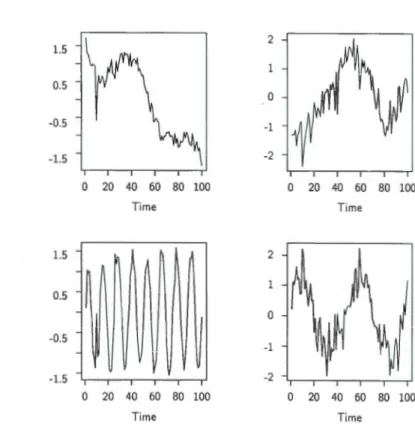
(sorne examples are shown in figure 1.1) :
1. A data set that mixes a disturbance pattern ( e.g. Rubina & McC<u·thy, 200L!) with
a linear or non-linear trends and sorne noise. To give a more realistic shape to tree
21
ring series. It's amplitude in x and y axis varies amongst series, as well as the first and last year of effect. With this set we will test if the different kind of trends are recovered as well as the disturbance pattern.
2. This set mixed a trend with large spikes. Theses spikes try to represent dist ur-bances affecting trees for only one or two years like a severe drought, ice storm ... The value of each spike is set as the mean of the series at the considered year plus x time the standard deviation (a} We will test the effect of varying amplitudes of spikes, as well as the effect of different nurnber of spikes on the detection of the spike.
3. In order to test spike threshold for the detection, 159 series were created. For this purpose the strategy is different. Ille have added to one series with one spike an increasing number of non spiky series to understand at what dilution a spike is still detected. The estimation of confidence intervals for the detection and recovery of spikes is not defined in an analytical way. Therefore, a bootstrap with 1000 permutations, when possible, was made. This re-sampling replaces the non spiky series then, ICA was restarted.
4. A set of complex data was generated in order to simulate real tree ring series by mixing a trend, disturbances, noise and a cyclicity pattern. The cyclicity was simulated using two sine waves simultaneously : a 12 years and a 60 years. This set was made of four different trends (two linear and two non-linear) containing 20 series each.
Our initial analyses revealed that under sorne conditions the ICA algorithm was unable to separate trends and cyclic patterns in the data. The principal problem is that there are more potential component to be extracted than there are series in the analysis. Unfortunately, ICA is not able to extract more component than the number of input series. To solve this problem, we propose to analyze trends by ICA separately (Figure 1.2). A classification method can used to separate series with different trends. Then a second ICA is performed on the four independent components representing the mixture of recovered trends and cycles. Two extractions have to be clone separately because
Series components Generated series 0 20 40 60 80 100 0 20 40 60 80 100 Ti me Ti me 0 20 40 60 80 100 0 20 40 60 80 100 Ti me Ti me 0 20 40 60 80 100 0 20 40 60 80 100 Ti me Ti me
Figure 1.1 Example of constructed series with the components used to build it. The
component column shows from top to bottom a disturbance pattern, then linear trends
and non-linear trends. The right column shows sorne example of generated series with from top to bottom positive trended disturbances, then a spike with a trend and a non-linear trended disturbance.
Trend A
Spikes are removed to decrease complexity
Trend B Trend C Trend 0
Non spiky series
Figure 1.2 Analysis of complex series schematic representation
2:3
ICA provide statistically independent results. This independence mean that a second analysis cannot be clone on some component extracted from the same first analysis due to the laclc of interaction (different coordinates) between input data.
We used the FastiCA algorithrn (Hyviirinen & Oja, 2000) to do the ICA. This a lgo-rithm, after data are centered, projects the data onto an dirnensional space where n is the number of components to extract (specifiee! by the user). This algorithm usee! the fixecl-point iteration scheme for maximizing the neg-entropy with the constraints that the estimated un-mixing matrix is an orthonormal matrix. In practice Principal Com-ponent Analysis can be usee! as preprocessing tool for ICA in orcler to set the number of component to extract (Stone, 2004). However, in the case of constructecl data this pre-process is not necessary because we know a priori the number of components to extract. We, however, tested the usability of the PCA to set the number of components.
A comparison of ICA is made with the mean series which is a year to year mean of the series.
As a measure of the goodness of the ICA we used the surface recovered by series. vVe calculated the cornmon surface the original data (without noise) and the surface of the
ICA components. This was compared to the mean series (with noise).
1.4 RESULTS AND DISCUSSION
1.4.1 Trend Recovering within Data Set 1
ICA recovers the trends and disturbances of our data. However, these two pattern appears rnixed together in the sarne component (Figure 1.3). Moreover, further analysis shawn that this performance is better than that of a mean series for non-linear trends as shawn in figure 1.3, whereas mean series do better with linear trend. This comparison is given by the percent of common area between the recovered series (by ICA or mean) and the original series without noise (Table 1.1). With linem trend the ICA explained
is 17% less than a simple mean, while for non-linear trends the ICA was of 11% better
than a simple mean.
If series with the three different trends of the same kind (linear or non linear) are used as input data, ICA recovered them but seems to be unable to sepamte positive and
negative trends and the performance (measured again as common surface under the
mean curve) is less good than results of a single trend (Table 1.1), but fm· better than
the mean which erases the positive and negative trends.
Results of ICA done in the same way with non-linem· trends are much better than the mean of the series (Table 1.1), but it is just able to distinguish three trends of the four
trends present in the series and the perturbation pattern disappem·s like with the mean
series. When applied on all these data simult<meously, ICA recovered the same three non-linear trends and the perturbation pattern with a slightly positive trends. The series obtained by the mean is non-linear with the perturbation.
25
extract (Himberg & Hyviirinen, 2001; Stone, 2004) in a subsequent ICA. The main three
axis of the PCA explained 83% of the variance (result not shawn) of all data. Other axis did not explained a significant par of the variance (und er 2%). Consequently, an ICA with three components to extract was clone (Table 1.1). This wru; one component less
than there are signais in the simulated data. The analysis recovered two linear trends and the non linear which was not recovered when four components were extracted. Generally we observed that if we decreased the number of components to extract, the non linear trends extracted look like more and more the average non linear trend. It is probably good to try bath methods for real data. An extraction with the number of
components set by a PCA and an extraction with the maximum number of components
that can be obtained from the ICA. In arder to set a number of components to extract
equals to the number of source signal various methods exist and are discussed in Penny,
Roberts & Everson (2001) but in tree ring width the number of "anomalies" and other sources can be larger than the number of input series. Setting the number of component to extract equal to the number of input series can be a good idea.
1.4.2 Detection of Spikes and Recovery of Their Values within Data Set 2 and 3
As described before, our aim is to determine the minimum size of a spike that is detected and the minimum proportion of series that contain a spike required for spike detection. Also, we wanted to understand the consequences of having several spikes in a tree series
on the detection of a spike.
The detection threshold (Table 1.2) is as law as the definition of a spike used by us.
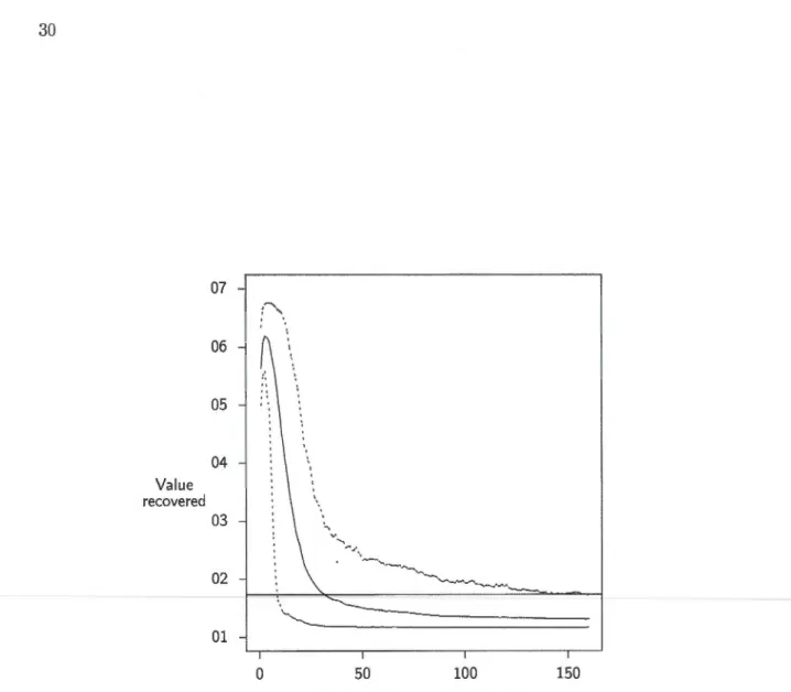
ICA always detected spikes as law as 40' that occur in 5 series. The lm·ger is a spike, the more easily it is detected, even if it occurs less frequently. Spikes of 40' were detected if they occur in 1/15 series, spikes of 50' in 1/16 and spikes of 100' in 1/128 (Table 1.2). This representation of spikes within series, in arder to be able to detect it, is effectively non-linear (Figure 1.4). ln arder to test more robustly this detection threshold, the detection of a single 100' spike was tested with an increasing number ( up to 160) of
4 '
-2 3 •' : ·~ 2 1 0 0 -1 -1 -3 0 20 40 60 80 100 0 20 40 60 80 100 Ti me Ti me 3 2 1 0 -1 -2 -3 0 20 40 60 80 100 0 20 40 60 80 100 Ti me Ti me 4 4 3 : ~2
~~:
~
.
~ ~.'.
0 : ' ~ ".;' "'<
-2 2 -1 -3 0 20 40 60 80 100 0 20 40 60 80 100 Ti me Ti meFigure 1.3 Results of the r covered trends and disturbance pattern. Dotted lines re
p-resent original components centered on the mean and plain lines represent the recovered components by the independent component analysis.
27
Tableau 1.1 Performance of the independent component analysis compared to a mean
series in trends and disturbance pattern recovering express by the proportion of surface recovered. Values shows how the analysis performed by comparing the share proportion of area under recovered curves with the original non noisy curve. Symbol " - " is use for series without trends, "
1 "
for positive trends, " \ " for negative trends, " r v/""'. " for linear trend becoming non linear, " /""'.r v " for non linear trend becoming linear, " /"""'. " for non linear hyperbolic trend and " D " for non linear " omega like " trend. " One " refers to a te::;t applied on just one trend, " Mix s.t. " refers to a test applied to all linear or all non linear trends and " Mix all " to a test applied to all trend at the same time. " - " shows non obtained results. PCA ICA shows results of ICA clone with the number of components to extract set by PCA.Linear trend Non Linear trend
Input
1
\
n
One ICA 0.621 0.775 0.723 0.872 0.880 0.760 0.781
One l\!Iean 0.691 0.909 0.936 0.777 0.807 0.663 0.612
Mix s.t. ICA 0.726 0.737 0.782 0.467 0.733
Mix s.t. Mean 0.734 0.774
Mix all ICA 0.630 0.801 0.425 0.729
Mix all Mean 0.828
non spiky series. Moreover, a bootstrap with 1000 permutations was used to calculate a confidence interval of the recovered spike's size. Bootstrap gave two results as shown in figure 1.4 : the value recovered vary by 2 units or more within the confidence interval and the detection is affcctcd by the noise. A value to be rccovcred of 100" has a maximum dilution of 1/8 series with a threshold of detection set at 125% the noise maximum value and sometime, it can be detected in 1/128 series. Our capacity to detect multiple spikes is not directly related to the magnitude of the spikes. In table 1.2 we compared results of a 50" spike versus the addition of one 40" and one 10" spike where detection works better with the 50". The ICA was always more able to detect a single large spike (e.g. a single spike of 50") than the detection of several simultaneous spikes of the same cumulative magnitude (e.g. two spikes of 2.50"). The sign of the spike (positive or negative) did not
affect the detection due to rotation if only one spike is present in the series. For two
spikes of opposite sign, the difference of sign between them is preserved. l\!Ioreover, ICA attempt untie, if possible, spikes in arder to recover each spike in a single component. In fignrc 1.5 wc have rccovcrcd fivc spikcs. Thcsc spikcs appcarcd at ycar 9, 1L 15, 25 and 41, and are mixed differently. In arder to untie each spike, the number of components to extract has to be set correctly. However, it is impossible to extract more components than the number of series in the analysis. The proximity of spikes ( e.g. one year between two spikes) did not affect their recovery as shawn in figure 1.5 (top ww).
1.4.3 Complex Series Analysis of the Data Set 4
The analysis of simulated complex data gave similar results to the trend and distur -bances recovering tests. Spikes were recovered separately, but the other parts (trend,
cyclicity and disturbance) were mixed together. The principal problem is that there is
more potcntial component to be extracted than the number of data in the analysis.
Consequently, data were separated according to their trend and two ICA were made as
explain in the methods. Results of this second analysis (Figure L6) show that it was
able to recover the two cyclicity patterns. However, the trends are in two components as a mix of a linear trend and a non-linear trend whereas we were expecting to have six
- -- - - - -
---l
29Tableau 1.2 Results of the detection of spikes in a set of series without spikes by the independent component analysis. Nb. Spike give the number of spike involved at the
same year, a Add. referred as the number of time the standard deviation is added with
Val. the value in the input matrix. Nb. S. referred to the number of series used in the analysis. Val. Rec. is the absolute value of the spike recovered. Mean, Sd., Max and Min referred to the mean, the standard deviation, the maximum value and the minimum value without the spike of the recovered series.
*
give the detection threshold, which is in reality 1/(Nb. S.). The first line of data gives the characteristics of other values at thesame year than the spike, and the second line reproduce the same values but centered
on the mean.
Nb. Spikes a Add. Val. Nb. S. Val. !lee. Mean Sd. Max Min One 4a 2.51 5 3.17 -0.03 0.96 2.12 -2.11 One 5a 2.79 5 3.76 -0.04 0.93 2.07 -2.12 One 6a 3.07 5 4.56 -0.05 0.89 1.83 -1.80 One 7a 3.35 5 5.12 -0.05 0.86 1.73 -1.73 One Sa 3.63 5 5.62 -0.06 0.83 1.63 -1.67 One 9a 3.91 5 6.06 -0.06 0.80 1.55 -1.60 One lOa 4.19 5 6.45 -0.06 0.77 1.47 -1.55 One lla 4.47 5 6.80 -0.07 0.74 1.37 -1.46 One 4a 2.51 5 3.24 -0.03 0.95 1.95 -2.08 One 4a 2.51 10 2.97 -0.03 0.96 2.10 -2.25 One 4a 2.51 15* 2.90 -0.03 0.97 2.38 -2.22 One 5a 2.79 5 4.11 -0.04 0.92 2.00 -1.84 One 5a 2.79 10 3.38 0.03 0.95 2.28 -1.97 One 5a 2.79 16* 3.22 0.03 0.96 2.30 -2.17 One lOa 4.19 10 6.53 0.00 1.01 1.85 -1.76 One lOa 4.19 20 6.71 0.01 1.00 1.85 -1.85 One lOa 4.19 100 4.76 -0.05 0.96 2.67 -2.14 One lOa 4.19 128* 3.40 -0.03 0.95 2.85 -2.23
Two 4a & la 2.51 & 1.67 5 3.12 -0.03 0.97 2.07 -2.14 Two 4a & 2a 2.51 & 1.95 5 3.17 -0.03 0.96 1.95 -2.04
Two 4a & 3a 2.51 & 2.23 5 3.35 -0.03 0.95 1.92 -1.97 Two 4a & 4a 2.51 & 2.51 5 3.68 -0.04 0.94 2.07 -1.85
Two 4a & 5a 2.51 & 2.79 5 4.36 -0.04 0.91 2.07 -1.71 Two 4a & 6a 2.51 & 3.07 5 4.98 -0.05 0.87 2.07 -1.76 Two 5a & 6a 2.79 & 3.07 5 5.23 -0.05 0.86 2.04 -1.68
Value recovered 07 05 04 03 02 01 0 · ...
·-50 100 150Number of series in the analysis
Figure 1.4 Recovering of one spike with increasing number of series without spike.
The plain line represents the mean and dotted lines the 90% confidence obtained by
bootstrap with 1000 permutations when possible. The vertical line gives the threshold
31 Recovered series 0 20 40 60 80 100 0 20 40 60 80 100 Ti me Ti me 0 20 40 60 80 100 0 20 40 60 80 100 Ti me Ti me 0 20 40 60 80 100 0 20 40 60 80 100 Ti me Ti me 0 20 40 60 80 100 0 20 40 60 80 100 Ti me Ti me
1.5 0.5 -0.5 -1.5 0 20 1.5 0.5
r
-0.5 -1.5 0 20 40 60 80 Ti me 40 60 80 Ti me 2 0 -1 -2 100 100 0 20 40 60 80 100 Ti me 0 20 40 60 80 100 Ti meFigure 1.6 Resulting trend and cycle of independent components extracted during the analysis of complex simulated data
different trends recovered.
1.5 CONCLUSION
Independent component analysis is a relatively new statistical methodology It success in medical science for the electroencephalographic brain dynamics had show the power of the methods applied to time series (Vigario et al., 1998; Hyviirinen, Karhunen & Oja, 2001). However, their is major differences in the kind of analysis made with e
lectroen-cephalographic and the dendrochronological approach. In climate dendrochronology we are interested in all extracted components, like in financial analysis, whereas medi-cal science seek for anomalies and more generally spikes detection. Recently, ICA bas been applied to try to uncover hidden patterns in the observed financial data (Back
33
(Ham & Faour, 1999) which is closely related to our goal in tree ring width analysis. In this paper multiple tests have been done to test the applicability in dendrochronology. Like in medical science spike recovering is done without problems. Moreover, ICA seems
to improve trends and large disturbance detection in comparison with the classical
mean series made in dendrochronology approach. Where ICA improve tree ring width
analysis is in the recovering of cyclicity and it seerns to be an efficient method to recover disturbance. Whereas classical analysis try to identify such patterns with the
estimation of parameters in hypothetical relationship, ICA extract it directly. This direct
extraction will permit to work on other independent components or on this cyclicity
without the offset introduced by their estimation. Moreover, the recovered patterns
are statistically independent, which can be of great interest especially for detecting co -occurring disturbances. Also a mean tre ring width series can be obtained without
disturbance effect which can be precious for studies dealing with long tenu trends. In the applicability of ICA for particular contexts lies the power of this technique for
tree ring research. In particular, spike recovering can improve the resolution of insect
DE LA THÉORIE À
L
A
PR
A
TIQ
UE
Le premier chapitre nous a permis de tester une nouvelle méthode pour l'étude des cernes de croissance des arbres. Différents tests furent appliqués sur des données simulées, avec succès. Mais, un test sur de vraies données doit être fait avant d'aller plus loin. Pour cela nous avons utilisé des données provenant de trois articles scientifiques qui utilisent les cernes pour détecter les épidémies d'insectes passées. Nous espérons ainsi obtenir les mêmes résultats et voir si notre méthode ne pourrait pas aboutir à une recherche plus affinée dans ce domaine.
CHAPITRE II
IDENTIFYING INSECT OUTBREAKS : A COMPARISON OF A
BLIND-SOURCE SEPARATION METHOD WITH HOST VS
NON-HOST ANALYSES
The identification of past insect outbreaks is often determined using a comparison of
host and non-host tree-ring growth chronologies. Yet this may be a problern when no
n-hosts are either affected by the outbreaking insect or when the growth of host and
non-host trees does not respond sirnilarly to the sarne climatic factors. In this paper, we
investigate the use of a blind source separation rnethod to identify past outbreaks. This
method, used in neurology and called independent components analysis (ICA), directly
identifi.es disturbance patterns in time series data. vVe re-analyzed the tree-ring data
from three papers dealing with insect outbreal<S for which data were available. These
papers focus on western spruce budworm, pandora rnoth and Douglas-fir tussock moth
outbreaks. We compared the results of the original analyses in these papers conducted
using a comparison of tree growth in host and non-host trees with results from ICA.
We detected the five outbreaks identified in the original papers using the ICA for host
series. However, the start and end dates for the outbreaks were different in 75% of the
ICA analyses compared to the dates reported in the original paper. On the other hand,
we were able to detect growth reduction in non-host ponderosa pine chronologies during
western spruce budworm outbreal<S with generally 50% of the trees affected by a growth
reduction for the considered site. Other non-host clu·onologies tended to show increased