Random monotone operators and application to stochastic optimization

(1)

HAL Id: tel-01960496

https://pastel.archives-ouvertes.fr/tel-01960496

Submitted on 19 Dec 2018

HAL is a multi-disciplinary open access

archive for the deposit and dissemination of sci-entific research documents, whether they are pub-lished or not. The documents may come from teaching and research institutions in France or abroad, or from public or private research centers.

L’archive ouverte pluridisciplinaire HAL, est destinée au dépôt et à la diffusion de documents scientifiques de niveau recherche, publiés ou non, émanant des établissements d’enseignement et de recherche français ou étrangers, des laboratoires publics ou privés.

Random monotone operators and application to

stochastic optimization

Adil Salim

To cite this version:

Adil Salim. Random monotone operators and application to stochastic optimization. Optimiza-tion and Control [math.OC]. Université Paris-Saclay, 2018. English. �NNT : 2018SACLT021�. �tel-01960496�

(2)

NNT

:

2018SA

CL

T021

Op ´erateurs monotones al ´eatoires

et application `a l’optimisation

stochastique

Th èse de doctorat de l’Universit é Paris-Saclay pr épar ée à T él écom ParisTech Ecole doctorale n◦_{580 Sciences et technologies de l’information et de la}

communication (STIC) Sp ´ecialit ´e de doctorat : Automatique, Traitement du Signal, Traitement des Images, Robotique

Th èse pr ésent ée et soutenue à Paris, le 26/11/2018, par

A

DIL

S

ALIM

Composition du Jury :

Antonin Chambolle

Directeur de recherche CNRS, Ecole Polytechnique Pr ´esident

J ´er ˆome Bolte

Professeur, Universit ´e Toulouse 1 Capitole Rapporteur

Bruno Gaujal

Directeur de recherche INRIA, Laboratoire d’Informatique de Grenoble Rapporteur

Panayotis Mertikopoulos

Charg ´e de recherches CNRS, Laboratoire d’Informatique de Grenoble Examinateur

Walid Hachem

Directeur de recherche CNRS, Universit é Paris-Est Marne-la-Vall ée Directeur de th èse

Pascal Bianchi

Professeur, T él écom ParisTech Co-directeur de th èse

J ´er ´emie Jakubowicz

Chief Data Officer, Vente-privee Invit ´e

Eric Moulines

(3)

Remerciements

Tout d’abord, je remercie mes directeurs de thèse, Pascal et Walid pour m’avoir proposé ce beau sujet et pour m’avoir encadré pendant ces trois années. J’ai eu de la chance de tomber sur vous. On aura passé de bons moments à parler approximation stochastique à "l’heure où on démontre les théorèmes facilement" ou en déplacements à Troyes, Bordeaux, Nice... Merci pour votre bienveillance, votre patience et votre aide pour ma recherche de postdoc. J’ai énormément appris à vos côtés. Je te remercie également Jérémie, pour m’avoir permis d’eﬀectuer cette thèse et ainsi que pour ta gentillesse et le soutien matériel que tu m’as apporté.

Je remercie vivement Jérôme Bolte et Bruno Gaujal d’avoir accepté de rapporter cette thèse. Merci également à Antonin Chambolle, Panayotis Mertikopoulos et Eric Moulines d’avoir accepté de faire partie du jury. Présenter mes travaux devant vous tous est un grand honneur.

I would also like to thank Volkan Cevher and Peter Richtarik for accepting to host me at EPFL and at KAUST.

Enﬁn, je te remercie Olivier Fercoq pour l’aide précieuse que tu m’as apporté.

J’ai croisé beaucoup de monde à Télécom. Alors je dédie cette thèse à mes amis et collègues de Comelec, Achraf, Akram (see u in Jeddah), Marwa, Mohamed, Mehdi, Julien, Xavier, Alaa, Hussein, Samet, Yvonne, Chantal, Hamidou et tous ceux que j’oublie. J’ai quitté Comelec à la suite d’une... disons restructuration pour venir travailler à TSI (hum IDS, pardon). Aussi, je tiens à remercier l’équipe que j’y ai trouvé. D’abord mes amis de l’ENSAE, Anna et Moussab, qui sont depuis six ans dans ma promotion. Il sera difficile d’énumérer tout ce qu’on a partagé ici (musique, maths, business, gossip, voyages, mariage...). Mais essentiellement, on fait ce qu’on sait faire, on monte des coups. Guillaume, nos discussions autour de l’optimisation, du rap et du soulevé de terre m’ont beaucoup apporté. Je te souhaite une belle carrière au sein de la franc-maçonnerie. Une spéciale pour le bureau des quatre. Huge, my BAI, RDV au Ghana. Ceux qui doivent entrer à Télécom par la fenêtre, Pierre A. (Calgary Yeah !) et Mathurin (Pouloulou). Et enfin Pierre L., l’homme de la situation, pour les fous rires et pour m’avoir installé Ubuntu. Tu as changé le cours de ma thèse ;). Salutations à Mastane tah les numbers one et Massil de Montréal Rive Sud 94230 t’entends? Dédicasse à Gabriela et Robin pour sa sagesse en termes d’altérophilie et de ski. Big up aux anciens aussi, Nico et Mael (je veux faire de l’oseiiillleeeee), Ray Bro (l’homme qui perd 2 fois son passeport en 1 voyage). J’en place une pour Albert aussi, merci de m’attendre haha. Sans oublier les nouveaux qui vont poursuivre dans les sillons de l’approximation stochastique, Anas (soit solide !) et Sholom, le thésard de nuit. Profitez bien ! Enfin, je ne peux pas terminer ce paragraphe sans passer par la start-up (Alexandre : merci pour les conseils, Alex : préviens moi quand tu retournes à Tahiti, ça m’intéresse, Hamid : on se fera un voyage aux US un jour, ça va être drôle) et par les contrées plus reculées de Télécom, Tom (qui devrait devenir docteur quelques heures après moi, normalement), Valentin et Kevin (cesse de raconter des bêtises).

Je dédie également cette thèse à la communauté scientiﬁque que j’ai cotoyé, les profs de Télécom (Robert, Umut, François, Ons, Joseph, Slim, Alexandre, Stéphan, Olivier), les personnes que j’ai ren-contré en conférence (Guillaume, Gabor, ...), ceux qui sont venu squatter (Noufel, Loic), les anciens de

(4)

l’ENSAE (Mehdi, Alexander, Badr, Vincent, Pierre A.), d’Orsay (Henri) et Florian, qui m’a donné le goût de la recherche. Je remercie également les profs (avec une mention spéciale pour M. Patte) qui m’ont fait aimé cette discipline, les mathématiques.

Ces trois années m’ont aussi permis de m’initier à diﬀerents sports, tels que l’escalade avec Arnaud ou le JJB avec–My nigga My nigga–Ams Warr Sow Pastore, Aket dit le Jardinier et tous les membres du club, Hos !

Un grand merci à mes amis ! Du Hood à l’école en passant par la prépa et Stralmi, on a fait du chemin ! J’ai plein de souvenirs qui me viennent en tête à cet instant. On en aura des choses à raconter en vieillissant. Big up à la team Very Bad Trip, Rich Gang (Arnold, tu es le prochain sur la liste), Niggaz in Paris, Revna, Prémices et les Expats. Madjer, je n’ai pas osé mettre ta citation au début, mais j’y ai pensé fort. J’ai également une pensée pour Marcel, et ceux qui nous ont quitté. Enﬁn, une mention spéciale pour mon compagnon d’infortune Sami, et le physicien fou Quentin.

Enfin je souhaite dédier cette thèse à ma famille. Ma famille au sens large, le groupe Famille et ma belle-famille. Merci à ma belle-mère et ma belle-famille de nous soutenir au quotidien, vous êtes d’une aide précieuse et on a de la chance de vous avoir. Je rejoins Abi et Abdullah au rang de docteur. Zaki et Houssam, je vous souhaite toute la réussite pour la suite. Je dédie cette thèse à mes oncles Schubert et Zaidou, mon cousin Aouad et mes nièces Naïma et Aya. Enfin, à mon frère Irfane qui m’a montré le chemin, mon père, et ma mère qui m’a toujours soutenu et couvert pour que je puisse étudier sans me soucier du reste. Voilà la récompense pour tes sacrifices. Finalement j’embrasse mon épouse Kawtar qui me supporte au quotidien :). Je suis très heureux d’avoir partagé ces dernières années à tes côtés et je garde d’excellents souvenirs de cette période riche en voyages, délires et émotions. Que cela dure ! Mais attention : c’est fini les t-shirts à fleurs haha ! La vie nous a fait un magnifique cadeau qu’on a appelé Imrane et que j’embrasse également. Merci de m’aider à me lever le matin.

(5)

Chapter 1 Introduction

1.1 Theoretical context : Stochastic Approximation

In the fields of machine learning, statistics or signal processing, many methods rely on an underlying optimization algorithm. In modern applications of data science, it is often not possible to run these algorithms on a single computer. Indeed, when a large amount of data has to be processed, or when streams of data arrive online, either classical algorithms need to be simplified or several computers have to be used. These modifications of classical algorithms can often be formalized by the introduction of randomness in the iterations. To see this, first consider the case of big data problems. Since each iteration of classical algorithms would process the whole dataset, simplified versions of these algorithms will rather process a small randomly chosen amount of data at each iteration. Then, when this task is tackled by a connected network of computing agents, there must be communications inside the network to solve the problem. These communications are often required to happen randomly in the network if it is large. Moreover, in practical settings, the agents compute and communicate only at random instants. Finally, online learning problems need a full knowledge of the distribution of the data to be solved completely. Since streams of data arrive online, the distribution of the data is revealed across time to the user through random realizations. In other words, solving online learning problems requires to be able to work in noisy environments. The algorithms used in the contexts mentioned above can be formalized as optimization algorithms for which the function to minimize is unknown but revealed across the iterations. The literature of stochastic optimization, which studies these algorithms and which this thesis belongs, lies at the intersection of the mathematical optimization and the literature of stochastic approximation. Stochastic optimization algorithms find numerous applications in signal processing and machine learning [34]. Since the seminal work of Robbins and Monro [99] in 1951, stochastic optimization algorithms are analyzed through the prism of the stochastic approximation literature. We start by briefly recalling the goal of stochastic approximation algorithms.

1.1.1 Robbins-Monro algorithm

The stochastic approximation literature studies algorithms that take the form

xn+1 = xn+ γn+1h(ξn+1, xn) (1.1)

where xn are random vectors valued in some Euclidean space X, (ξn) is a sequence of random variables

(r.v) valued in a measure space Ξ, (γn)n is a sequence of positive step sizes and h : Ξ × X → X is

(10)

The aim of the algorithm is to ﬁnd a zero of the expectation function H(x) = Eξ1(h(ξ1, x)) assumed

to exist, i.e an element x ∈ X such that H(x) = 0. Denote as Z(H) the set of zeros of H. Under some assumptions on h and the step sizes (γn), it is known that (xn) converges to Z(H). The strength

of stochastic approximation algorithm (1.1) is to be able to ﬁnd a zero of H without evaluating the expectation H(x). Indeed, in many applications, the computation of H is intractable. There is a Law of Large Number eﬀect that allows to smooth the randomness. A widely studied example of Robbins-Monro algorithm (1.1) is the stochastic gradient algorithm.

Example 1. The stochastic gradient algorithm aims at ﬁnding a minimizer of a diﬀerentiable function F: X→ R. The function F is itself written as an expectation with respect to (w.r.t.) some r.v ξ

F(x) = Eξ(f (ξ, x)), (1.2)

where f(ξ, ·) is a diﬀerentiable. The stochastic gradient algorithm update is written

xn+1 = xn− γn+1∇f(ξn+1, xn) (1.3)

where the gradient ∇f is taken w.r.t. the second variable (x), (ξn) is a sequence of i.i.d copies of ξ and

(γn) is a sequence of positive step sizes. Algorithm (1.3) can be cast as an instance of (1.1) by setting

h _{≡ ∇f. If f(s, ·) is convex, the following interchange property holds H(x) = E}ξ(∇f(ξ, x)) = ∇F(x)

for every x ∈ X. Since F is convex, Z(H) = arg min F. Under mild assumptions, the sequence (xn)

converges to an element in arg min F.

Two regimes that require diﬀerent tools can be considered to analyze stochastic approximation al-gorithms : the case where γn →n→+∞ 0 and the case where γn ≡ γ > 0. Typically, in the so-called

decreasing step sizes case (ﬁrst case), the sequence (xn) of iterates converges almost surely (a.s.) to a

zero of H. In the constant step size case (second case), the iterates quickly reach a small neighborhood of the set of solutions Z(H) in a burn-in phase, and then ﬂuctuate around the set of zeros. The main advantage of the decreasing step sizes case is to exhibit the a.s. convergence of the iterates. Although the constant step size case lacks the a.s convergence in general, the use of a constant step size is often more suitable in online learning settings.

A standard method to study evolution equations like (1.1) is the Ordinary Diﬀerential Equation (ODE) method, which was introduced in the 70’s by Ljung [79] and extensively studied by Kushner and coworkers (see e.g. the book [73]). This method allows to study the dynamical behavior of stochastic approximation algorithms and to prove their convergence. Assume that H is a Lipschitz continuous function over X and consider the unique diﬀerentiable function x : R+ → X such that x′(t) = H(x(t))

(where x′ _{denotes the derivative of x) starting at some prescribed value a ∈ X : x(0) = a. The ODE}

method relies on relating the iterates xn and the function x. More precisely, (xn) is seen as a noisy Euler

discretization of the function x.

1.1.2 A general framework

In this thesis, we develop a more general framework for stochastic approximation because the frame-work (1.1) fails to cover some important applications, see Sec. 1.2. Consider the following evolution equation

xn+1 = xn+ γhγ(ξn+1, xn) (1.4)

where the step size γ > 0 is taken constant, (ξn) is i.i.d with distribution µ and hγ is a measurable

function indexed by γ. Let us assume in most generality that

(11)

where H : X → X is some function. If H is a Lipschitz continuous function and the convergence (1.5) holds uniformly for x in the compact sets of X, then the ODE method can be applied and we are let back to the situation of the previous paragraph. However, this kind of assumption is too restrictive in many contexts, especially those mentioned in Sec. 1.2 below. We shall focus on the case where the convergence does not hold for every x, is not uniform over compact sets, and above all, H is a set valued mapping instead of being single valued. We are therefore led to study more general stochastic approximation algorithms.

1.2 Motivations

1.2.1 Stochastic Proximal Point algorithm

A ﬁrst motivation for studying the general framework (1.4) comes from non smooth stochastic optimiza-tion. Consider a convex function G : X → (−∞, +∞] which is lower semicontinuous (lsc) and proper (we shall write G ∈ Γ0(X)). Denote ∂G(x) the set of all subgradients of G at x. The subdiﬀerential

∂G : X ⇒ X is a set valued function. Consider x ∈ X. The proximity operator [87] of G at x is the minimizer of the (strongly convex) objective function:

prox_γG(x) = arg min

y∈XG(y) +

1

2γkx − yk

2_, _(1.6)

where γ > 0, and the Moreau envelope [130] of G at x is the associated minimum value Gγ(x) = min

y∈XG(y) +

1

2γkx − yk

2_. _(1.7)

Moreover, the Moreau envelope is diﬀerentiable and its gradient is a 1/γ-Lipschitz continuous function that satisﬁes (see [12])

prox_γG = I_{− γ∇G}γ (1.8)

where I is the identity of X. The goal of the proximal point algorithm [82] is to ﬁnd a minimizer of G (equivalently a point x such that 0 ∈ ∂G(x), called hereafter a zero of ∂G) by iterating

xn+1= proxγG(xn), (1.9)

where γ > 0. It is known that the sequence (xn) converges to a minimizer of G. The proximal point

algorithm enjoys good stability properties, among which exhibiting convergence for any γ > 0. The main drawback of this algorithm is that each iterate is implicitly deﬁned, i.e one has to solve an optimization problem to ﬁnd xn+1. This operation can often be costly. Although the proximity operator of some

classical functions has a closed form1_{, the proximal point algorithm is not practical in many cases.} A way to simplify the iterations is to represent G(x) = Eξ(g(ξ, x)) where g(ξ,·) is a convex function

and to apply the constant step stochastic proximal point algorithm [22, 121]:

xn+1 = proxγg(ξn+1,·)(xn), (1.10)

where γ > 0 and (ξn) are i.i.d copies of ξ. This algorithm can be seen as a generalization of the splitting

algorithm of Passty [94] to inﬁnitely many functions. Many loss functions used in machine learning can be

1

(12)

written as expectations G(x) = Eξ(g(ξ, x)) for which prox_γg(ξ,·) is easily computable whereas neither G

nor proxγG can be evaluated. A typical situation is the case where these loss functions boil down to ﬁnite

sums G(x) = N−1PN

i=1g(i, x) and proxγg(i,·) can be easily computed but proxγG is intractable. This is

e.g. the case for the classiﬁcation problems like Support Vector Machine (SVM) or logistic regression. Another example comes from distributed optimization in the context where a network of computing agents is required to minimize a "global" cost function G = N−1P

ig(i,·), under the restriction that

the "local" cost function g(i, ·) is only known by the agent i. Hence, the network can only perform local computations involving each agent i and their respective cost function g(i, ·) separately. In all these situations, the proposed algorithm is an instance of (1.10) where ξ is a uniform r.v. over {1, . . . , N}.

Note that (1.10) can be cast in the form (1.4) by setting hγ(s, x) = −∇gγ(s, x), where gγ(s,·) is

the Moreau envelope of g(s, ·). In this case, H = ∂G is set valued.

1.2.2 Stochastic Proximal Gradient algorithm

In optimization algorithms, proximity operators are often used to handle regularizations or constraints. In these cases, the problem to be solved is

min

x∈X F(x) + G(x),

where G ∈ Γ0(X) is a convex function and F is assumed diﬀerentiable. The proximal gradient algorithm

generalizes the proximal point algorithm (1.9) and is written

xn+1 = proxγG(xn− γ∇F(xn)), (1.11)

where γ > 0. If ∇F is Lipschitz continuous (we shall say that F is smooth), if F is convex and if γ is enough small, then it is known that (xn) converges to a minimizer of F + G. A ﬁrst instance of

this algorithm is the projected gradient algorithm to solve min_CF. This algorithm can be seen as an application of (1.11) by setting G = ι_C, where ι_C the convex indicator function of the convex set C. In this case, proxG = ΠC is the projector onto C. Each iteration of this algorithm requires to evaluate

the projection Π_C, which is sometimes intractable. However, the set C can often be represented as an intersection of simpler convex sets Cs, i.e C =T_s∈ΞCswhere projections onto Cs can be easily computed.

Another instance of the proximal gradient algorithm comes from structured problem in which G is a regularization term. The function G is represented as G =Pig(i,·), where proxγG is hard to compute

but prox_γg(i,·) can be evaluated. This is e.g the case for the overlapping group lasso : G(x) =PikxSik

where X = RN_{, the S}

i are subsets of {1, . . . , N} and xSi is the restriction of x to Si. This is also the

case for the total variation regularization : G(x) =P_{i,j}∈E_{kx(i) − x(j)k where G = (V, E) is a graph,} with V the set of nodes and E the set of edges, and where x ∈ RV_{. In all these examples, the proximal}

gradient algorithm cannot be implemented because it involves the computation of proxγG. However, in

all these examples G can be seen as an expectation w.r.t. some r.v. ξ, G(x) = Eξ(g(ξ, x)) (where the

expectation sometimes boils down to a ﬁnite sum). In general, the stochastic proximal gradient algorithm aims at minimizing F(x) + G(x) = Eξ(f (ξ, x)) + Eξ(g(ξ, x)) by iterating [24, 2,3]

xn+1= proxγg(ξn+1,·)(xn− γ∇f(ξn+1, xn)). (1.12)

This algorithm can be cast in the form (1.4) by setting hγ(s, x) =

1

γ(proxγg(s,·)(x− γ∇f(s, x)) − x).

(13)

1.2.3 Stochastic Douglas Rachford algorithm

When minimizing a sum of two convex functions F + G, the Douglas Rachford algorithm [78] enjoys more numerical stability than the proximal gradient algorithm at the cost of implementing a proximity operator for F instead of a gradient. Moreover, any positive constant step size can be used in Douglas Rachford iterations to converge to a minimizer. In order to design an algorithm that enjoys the good features of Douglas Rachford algorithm without the iteration complexity, we are interested in the stochastic Douglas Rachford algorithm with constant step size, in which the proximity operator of F (resp. G) is randomized. To this end, F and G are represented as expectations, as in Sec.1.2.2and the resulting stochastic Douglas Rachford algorithm is also covered by our general framework (1.4).

1.2.4 Monotone operators and Stochastic Forward Backward algorithm

Maximal monotone operators are set valued functions that generalize the subdifferentials [12,36]. Many optimization problems can be reformulated as finding zeros of a monotone operator (which is not neces-sarily a subdifferential). In this respect, the Forward Backward (FB) algorithm is a further generalization of the proximal gradient algorithm. The goal of this algorithm is to find a zero of a sum of two maximal monotone operators.

In this thesis, we refer to an operator as a set valued function A : X ⇒ X. The inverse operator A−1 _is

deﬁned by the relation y ∈ A(x) ⇔ x ∈ A−1_{(y). An operator A is said monotone if}_{hy − y}′_{, x}_{− x}′_{i ≥ 0}

as soon as y ∈ A(x) and y′ _{∈ A(x}′_{). Under a maximality condition [}₈₅_{] of A, the resolvent of A,}

Jγ = (I + γA)−1 is a single valued function. In this case, A is called a maximal monotone operator

and Jγ is a contraction deﬁned on X. Maximal monotone operators generalize subdiﬀerentials of convex

functions and resolvents generalize proximity operators. Indeed, A = ∂G is a maximal monotone operator if G ∈ Γ0(X), and its resolvent is proxγG. For every γ > 0, the Yosida approximation of A is deﬁned by

A_γ = _γ1(I − Jγ). Using (1.8), it is immediately seen that Aγ = ∇Gγ if A = ∂G. The set of zeros of A

is deﬁned to be Z(A) = A−1_{(0). Many problems in optimization can be reformulated as ﬁnding a zero}

of a maximal monotone operator. For example, in the subdiﬀerential case, Z(∂G) = arg min G. Given another maximal monotone operator which is single valued B, the Forward Backward algorithm aims at ﬁnding an element in Z(A + B) by iterating

xn+1 = Jγ(xn− γB(x)). (1.13)

If A and B are subdiﬀerentials, the Forward Backward algorithm boils down to the proximal gradient algorithm. Under a so called cocoercivity assumption of B, this algorithm is known to converge to a zero of A + B if γ is small enough.

Beyond minimization problems, saddle points problems arise naturally in optimization and machine learning (see e.g [83]). We the saddle points problems are convex-concave, they can be reformulated as ﬁnding a zero of a sum of two monotone operators A + B [101]. In optimization, primal dual algorithms like Douglas-Rachford [78], ADMM [62], Chambolle Pock [42] or Vu Condat [51, 124] can be seen as (skillful) instances of the FB algorithm. This FB algorithm is applied to the convex concave saddle point problem of ﬁnding so called primal dual optimal points of the initial optimization problem.

In order to develop a stochastic version of these primal dual algorithms, we are interested in a stochastic version of the Forward Backward algorithm. To this end, we consider a new tool called a random monotone operator A(ξ, ·), i.e ξ is a r.v. and A(ξ, ·) is a maximal monotone operator. Measurability issues due to the fact that A is set valued will be treated in the next chapter. Denote Jγ(s,·)

(14)

operator B(ξ, ·) which is single valued. The constant step stochastic FB algorithm is written

xn+1= Jγ(ξn+1, xn− γB(ξn+1, xn)). (1.14)

The aim of the stochastic FB algorithm is to find a zero of the so called mean operator A(x) + B(x) = E_ξ_{(A(ξ, x)) + E}_ξ_{(B(ξ, x)). Integrability issues due to the fact that A(ξ, x) is a set-valued r.v. will be} treated in the next chapter, along with the definition of the expectation of a set-valued r.v. We just mention here the fact that in the subdifferential case A(s, x) = ∂g(s, x), under mild assumptions [102], E_ξ_{(A(ξ, x)) = ∂G(x) where G(x) = E}_ξ_{(g(ξ, x)) (we shall say that the interchange property holds). The} stochastic FB (1.14) can be cast into the framework (1.4) by setting hγ(s, x) = −B(s, x) − Aγ(s, x−

γB(s, x)) and H = A + B.

1.2.5 Fluid limit of parallel queues

Beyond stochastic optimization algorithms, the framework (1.4) can be used to study general Markov chains. For example the framework (1.4) is considered in [61] to study Markov chains with discontinuous drift. Using the notation of (1.4), this means that even hγ(s,·) is discontinuous. We give an application

example that comes from queueing theory. We are interested in establishing the long-run behavior of the number of users in a model of parallel queues. Users arrive at random instant in the queues and the queues are served following a prioritizing rule. After scaling the problem in order to study the so called ﬂuid scaled process [61], the evolution of the number of users in the queues ﬁts our framework (1.4).

1.3 Dynamics of Robbins-Monro algorithm

To better understand the methods used in this thesis, we get back to the Robbins-Monro algorithm of Sec. 1.1.1. We provide the main arguments behind the ODE method. We shall focus on the constant step case that will be of interest in the ﬁrst part of this thesis. More precisely, we study the evolution equation (1.1) with γn≡ γ > 0.

1.3.1 Known facts related with dynamical systems

Consider a Lipschitz continuous function H : X → X. Then, it is well known that for every a ∈ X, the ODE x′ _{= H(x) with initial condition x(0) = a admits an unique solution over R}

+ [73]. We denote by

Φ(a) this solution and abusively denote Φ(a)(t) = Φ(a, t) for every t_{≥ 0. It is known that Φ satisﬁes} the property of being a semiﬂow over X, i.e. Φ(·, s + t) = Φ(·, t) ◦ Φ(·, s) for every t, s ≥ 0. The essence of the ODE method is to study the behavior of the interpolated process obtained from the iterates (xn) of the algorithm (1.1) as being an approximation of the ODE solution. To perform this analysis,

some important notions related to the dynamics of the semiﬂow Φ need to be introduced. A probability measure π over X is called an invariant measure for Φ if π = πΦ(·, t)−1 _{for every t > 0. The set of}

invariant measures for Φ is denoted I(Φ). A point x ∈ X is said recurrent for Φ if x = limk→+∞Φ(x, tk)

for some sequence tk → +∞. The Birkhoﬀ center BCΦ of Φ is the closure of the set of recurrent points.

The celebrated Poincaré’s recurrence theorem [53, Th. II.6.4 and Cor. II.6.5] says that the support of any π ∈ I(Φ) is a subset of BCΦ. The goal of the two next sections is to prove that the sequence of

iterates (xn) deﬁned by (1.1) with a constant step size γn ≡ γ > 0 converges in probability to the set

BCΦ as n → +∞ and γ → 0. Indeed, BCΦ is often a set of interest while looking for zeros of H. For

(15)

.

γ

xa,γ(t)

.

Figure 1.1: The linearly interpolated process of the iterates with step size γ > 0.

1.3.2 Convergence of stochastic processes

Consider a sequence (xn) satisfying (1.1) with a constant step size γn ≡ γ > 0 starting from x0 = a.

Consider the linearly interpolated process of the sequence of iterates (see Fig.1.1) xa,γ _{over R}

+, piecewise

deﬁned for every t ≥ 0 by

xa,γ(t) = xn+ (t− nγ)

xn+1− xn

γ , t ∈ [nγ, (n + 1)γ), n ∈ N. (1.15) As a continuous time stochastic process, xa,γ _{can be seen as a r.v. in the space C(R}

+, X) of continuous

functions endowed with the topology of the uniform convergence over bounded intervals. The ODE method ﬁrst consists in showing that xa,γ _−→

γ→0 Φ(a) in distribution in C(R+, X) (i.e narrowly, see [14]).

In other words, one can show that for every T > 0, sup_{t∈[0,T ]}kxa,γ_(t)_{− Φ(a, t)k −→ 0 in probability as}

γ _{→ 0 under some prescribed assumptions.}

This important result does not suﬃce to characterize the long run behavior of the iterates i.e the case T = +∞. What is ultimately needed is the long-run behavior of the process xa,γ _{in terms of the}

(16)

1.3.3 Stability result

To characterize the long-run behavior of xa,γ_{, the sequence (x}

n) is viewed as a Markov chain with

transition kernel Pγ. The advocated stability result typically ensures that the set of invariant measures

for Pγ, γ ∈ (0, γ0) is relatively compact for some γ0 > 0. Under such a condition, the ﬁrst result on the

narrow convergence of xa,γ _{can be used to show that every cluster point of the invariant measures of}

the Markov chain as γ → 0 is an invariant measure for the semiﬂow Φ [60]. Using Poincaré’s recurrence theorem, such cluster points are supported by the Birkhoﬀ center BCΦ. A reformulation of this result is

the following : lim sup n→∞ 1 n + 1 n X k=0 P_(d(x_n_{, BC}_Φ_{) > ε)} _−→ γ→0 0. (1.16)

1.4 From ODE to Differential Inclusions

Motivated by the examples of1.2, we shall relax the classical assumptions used in the ODE method and study the framework (1.4) where H is allowed to be set valued. In this situation, the classical ODE is replaced with a Differential Inclusion (DI): ˙x ∈ H(x) deﬁned on the set of absolutely continuous functions over R+, where ˙x denotes the derivative of x deﬁned almost everywhere. Stochastic approximation

algorithms built on DI have recently aroused an important research eﬀort to which this thesis belongs [17,

80]. In this work, two kinds of DI with diﬀerent behaviors are of interest.

1. First, the case where H(x) is convex compact and not empty for every x ∈ X and H is upper semicontinuous [6] (usc) i.e for every a ∈ X, and for every open set U such that H(a) ⊂ U, there exists a neighborhood V of a such that x ∈ V ⇒ H(x) ⊂ U. Assuming that for every a ∈ X there exists a solution to the DI starting at a (this holds under a linear growth assumption on H), the solution is in general not unique and the semiﬂow associated to the DI is hence set valued [6]. This kind of DI is of interest in many applications including game theory, or queueing systems. 2. Second, the case where −H is a maximal monotone operator [36]. In this case, we considered in

particular the situation where the domain of H is strictly included in X, which is of obvious interest for many stochastic optimization algorithms.

1.5 Contributions

1.5.1 Convergence analysis with a constant step size

We ﬁrst focus on the analysis of constant step stochastic approximation algorithms having a DI as a limit. We shall study the case where (hγn(s, xn))n∈Nconverges to the set H(s, x) as n → +∞ if xn→ x

and γn → 0. The function H is represented as a set valued expectation H(x) = Eξ(H(ξ, x)). The set

valued expectation is formally deﬁned as a selection integral and generalizes the Lebesgue integral to set valued mappings, see Chap. 2. To study the dynamics of the iterates (xn) given by (1.4) we adapt the

general approach of Sec. 1.3 to DI ˙x ∈ H(x) in the usc case and the monotone case of Sec. 1.4, each case requiring a speciﬁc treatment and exhibiting a speciﬁc convergence result.

(17)

The upper semicontinuous case

In this case, H(s, ·) is assumed to be a proper (∃x ∈ X, H(s, x) 6= ∅) usc operator. We denote as Φ(a) the set of solutions to the DI ˙x ∈ H(x) starting at a. We assume that Φ(a) is not empty, and Φ can be seen as set valued ﬂow. Set valued analogues to classical dynamical systems results 1.3.1 will be considered. This framework is introduced in the paper [107] under the additional assumption that X is a compact space. In our work, we relaxed the compactness assumption, which extends the scope of the algorithm (1.4) to e.g., proximal non convex stochastic gradient algorithm 1.2.2, or queuing algorithms such as 1.2.5. Denote I(Φ) the set of invariant measures for the set valued ﬂow Φ, a notion introduced in [107]. Denoting d a distance that metricizes the topology over C(R+, X) of uniform convergence over

compact intervals, we ﬁrst prove the dynamical result sup

a∈K

P_(d(xa,γ_{, Φ(a)) > ε)}_−→

γ→0 0, (1.17)

for every compact set K ⊂ X and every ε > 0, where d(xa,γ_{, Φ(a)) denotes the distance from the function}

xa,γ _{to the set Φ(a). Under a stability assumption of the Markov chain (x}

n) this dynamical result is used

to characterize the long-run behavior of the iterates : lim sup n→∞ 1 n + 1 n X k=0 P_(d(x_n_{, BC}_Φ_{) > ε)} _−→_γ→0 _0, (1.18) where (xn) is the process satisfying (1.4) with step size γ > 0. Similar results involving the empirical

means xn= _n1Pnk=1xkare obtained. Finally, stability conditions based on the so-called Pakes-Has’minskii

criterion are provided in the context of the stochastic proximal non convex gradient algorithm (under a Łojasiewicz assumption [5, 30]) and in a model of parallel queues [61].

The monotone case

In this case, −H(s, ·) is assumed to be a maximal monotone operator with domain D(s) = {x ∈ X, H(s, x) 6= ∅}. If D(s) = X, then H(s, ·) is usc [97] and a dynamical result can be obtained from (1.17). We shall allow the domains D(s) to vary with s. This covers the contexts of the stochastic proximal point algorithm 1.2.1, the stochastic proximal gradient algorithm in the convex case 1.2.2, the Douglas-Rachford algorithm 1.2.3 and the stochastic Forward Backward algorithm 1.2.4. With a proof that explicitly leverages the maximal monotonicity of −H(s, ·) and allows the domains to be random, we ﬁrst show that

sup

a∈K∩D

P_(d(xa,γ_{, Φ(a)) > ε)}_−→

γ→0 0, (1.19)

where D is the domain of the mean operator H. Then, under a stability assumption of the Markov chain (xn), it is shown that if H satisﬁes the so called demipositivity assumption (see Chap. 2), then

lim sup n→∞ 1 n + 1 n X k=0 P_(d(x_k_{, Z(H)) > ε)}_−−→ γ→0 0 . (1.20)

Similar results that hold whether H is demipositive or not are obtained for the empirical means of the iterates. Finally, practical criteria ensuring the stability of the Markov chain (xn) are provided

in various instances of the stochastic Forward-Backward algorithm, including the stochastic proximal gradient algorithm of Sec. 1.2.2, the case where H(s, ·) is linear and monotone, etc.

(18)

.

γn

x(t)

.

Figure 1.2: The linearly interpolated process of the iterates with step sizes γn.

1.5.2 Applicative contexts using decreasing step sizes

Stochastic approximation with decreasing step sizes

The ODE method can also be used to study decreasing step sizes algorithm, i.e the evolution equa-tion (1.1) with γn→ 0. In this case, the linearly interpolated process x of (xn) over R+ with timeframe

γnis considered, see Fig.1.2. The general idea is to prove the almost sure convergence of the interpolated

process x to the solution of the ODE x′ _{= H(x). More precisely, the interpolated process is proven to be}

an almost sure Asymptotic Pseudo Trajectory (APT) of the ODE, a concept introduced by Benaïm and Hirsch in the ﬁeld of dynamical systems [15]. It is shown that d(x(t + ·), Φ(x(t))) →t→+∞0 a.s., where

we recall that d metricizes the topology of the uniform convergence over compact sets and where Φ is the semiﬂow associated with the ODE. Then, the asymptotic convergence of the sequence of iterates (xn) of the algorithm (1.1) can be obtained from the APT property. This notion has been generalized

to monotone DI in [24]. More precisely, the paper [24] studies the decreasing step size analogue of the stochastic Forward Backward algorithm (1.14)

xn+1 = Jγn+1(ξn+1, xn− γn+1B(ξn+1, xn)), (1.21)

where γn → 0. It is proven that the interpolated process of the iterates (xn) is an almost sure APT of

(19)

converges to an element of Z(H) as n → +∞ if −H is monotone and demipositive, and the sequence of empirical means (xn)n converges to a solution as n → +∞ whether −H is demipositive or not. In

this thesis, we proceed with Algorithm (1.21) in two directions. First, we apply this algorithm to solve a general composite optimization problem under linear constrains. The functions deﬁning the objective function and the matrices deﬁning the constraints are allowed to be represented as expectations, see Sec. 1.5.2below. Second, we generalize the stochastic proximal gradient algorithm with decreasing step sizes to solve a regularized optimization problem over a large and general graph, see Sec. 1.5.2 below. A fully stochastic primal dual algorithm

A ﬁrst example comes from primal dual optimization algorithms. Consider four convex functions F, G ∈ Γ0(X) and P, Q∈ Γ0(Z) where Z is an Euclidean space. Consider the following optimization problem:

min

(x,z)∈X×ZF(x) + G(x) + P(z) + Q(z) subject to Ax + Bz = c (1.22)

where A : X → V and B : Z → V are matrices with values in the Euclidean space V, and c ∈ V is a vector. In order to identify a minimizer of (1.22), primal dual methods typically generate a sequence of primal estimates (xn, zn)n∈N and a sequence of dual estimates (λn)n∈N jointly converging to a saddle point

((x, z), λ) of the Lagrangian function associated with (1.22). Under some qualiﬁcation condition, (x, z) is a solution of Problem (1.22) and λ is a solution of a dual formulation of (1.22). The formulation (1.22) encompasses the formulation of classical primal dual algorithms [62, 42, 51, 124]. In these algorithms, F, P are treated explicitly (i.e through their gradient) and G, Q are treated implicitly (i.e through their proximity operator). We shall focus on the case where all functions to be minimized are given as statistical expectations, as well as the matrices and the vector deﬁning the linear constraints. In other words, F(x) = Eξ(f (ξ, x)) where f (ξ,·) is a convex function. A similar representation is allowed for G, P

and Q. Besides, A = E(A) where A is a random matrix. A similar representation is allowed for B and c. These expectations are unknown but revealed across the time through i.i.d realizations. Only stochastic (sub)gradients or stochastic proximity operators are available to the user. To solve this problem, we ﬁrst remark that saddle points of the Lagrangian can be seen as zeros of a sum of two well chosen maximal monotone operators which are given as a set valued expectations. Hence, the stochastic FB algorithm can be applied and leads to a converging algorithm. To our knowledge, the proposed algorithm is the ﬁrst fully stochastic primal dual algorithm. Application to distributed and asynchronous optimization will be considered.

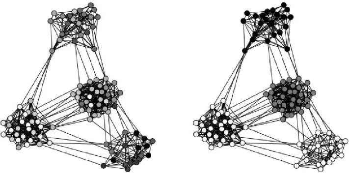
Online regularization over large graphs

Consider a graph G = (V, E) where V is the set of vertices and E is the set of edges. We ﬁrst consider the resolution of the following programming problem

min

x∈RVF (x) + TV(x, G) (1.23)

where F ∈ Γ0(RV) and TV(x, G) = P_{i,j}∈E|x(i) − x(j)| is the Total Variation regularization over

the graph G. When applying the proximal gradient algorithm to solve this problem, there exist quite affordable methods to implement the proximity step in the special case where the graph is a simple path without loops. However, when the graph is large and unstructured, the computation of the proximity operator is more difficult. To overcome this difficulty, we introduced an algorithm that we called "Snake" and that consists in randomizing the proximity operator in such a way that it becomes computable. More

(20)

precisely, Snake selects random simple paths in the graph and performs the proximal gradient algorithm over these simple paths. Hence, only proximity operators over simple paths are computed and Snake take beneﬁts of existing fast methods. Then, Snake is generalized to any regularization term tied to the graph geometry for which there exists fast methods to compute the proximity operator over a simple path. Snake is an instance of a generalization of the stochastic proximal gradient algorithm, whose convergence is proven. Numerical experiments are conducted over large graphs.

1.6 Outline of the Thesis

The next chapter is an introduction to some important notions used in the thesis. Then, the first part of the thesis studies the stochastic approximation framework (1.4) with a constant step size, mainly from a theoretical point of view. It consists in three chapters. Chapter 3 is related to Differential Inclusion involving an upper semicontinuous operator, and is based on the publication [28]. In Chapter 4, an analysis of the stochastic Forward Backward algorithm is performed, based on [25,26,27]. In Chapter5, the stochastic Douglas Rachford algorithm is studied and applications to structured regularization and distributed optimization is considered. This chapter is based on the papers [89, 111] and the technical report [110]. Applications of stochastic approximation algorithms with decreasing step size are considered in the second part of the thesis. After recalling the main ideas behind the proof techniques in Chapter6, we first consider a fully stochastic primal dual algorithm in Chapter 7, based on the work [112]. Finally, we provide an application to solve regularized problems over graphs in Chapter 8 ([109, 113, 114]). Chapter 9is devoted to a conclusion. The technical report [110] can be found in the Appendix A.

(21)

Chapter 2 Preliminaries

2.1 General notations

If E is a topological space, the Borel σ-field of E is denoted as B(E) and the set of probability measures on E endowed with its Borel field is denoted M(E). If (Ξ, G , µ) is a probability space and X and Euclidean space endowed with its Borel σ-field, the Banach space of measurable functions ϕ : Ξ → X such that kϕkp _{is µ-integrable (for p ≥ 1) is denoted L}p_{(Ξ, G , µ; X). The notation C(E, F ) is used to}

denote the set of continuous functions from E to the topological space F . The notation Cb(E) stands

for the set of bounded functions in C(E, R).

We use the conventions sup ∅ = −∞ and inf ∅ = +∞. Notation ⌊x⌋ stands for the ﬂoor value of x. If (E, d) is a metric space, for every x ∈ E and S ⊂ E, we deﬁne d(x, S) = inf{d(x, y) : y ∈ S}. We say that a sequence (xn, n ∈ N) on E converges to S, noted xn →n S or simply xn → S, if

d(xn, S) tends to zero as n tends to inﬁnity. For ε > 0, we deﬁne the ε-neighborhood of the set S as

Sε := {x ∈ E : d(x, S) < ε}. The closure of S is denoted by cl(S), and its complementary set by

Sc_{. The characteristic function of S is the function} _✶

S : E → {0, 1} equal to one on S and to zero

elsewhere. If E is an Euclidean space, the convex hull of S is denoted by co(S).

2.2 Set valued mappings and monotone operators

Consider an Euclidean space X. We recall some basic facts related with set valued mappings and their associated diﬀerential inclusions with emphasis on maximal monotone operators over X. These facts will be used in the proofs without mention. For more details, the reader is referred to the treatises [40], [12], [6], [36], or to the tutorial paper [96].

2.2.1 Basic facts on set valued mappings

Consider a set valued mapping (or operator) H : X ⇒ X, i.e., for each x ∈ X, H(x) is a subset of X. The domain and the graph of H are the respective subsets of X and X × X deﬁned as dom(H) := {x ∈ X : H(x)_{6= ∅}, and gr(H) := {(x, y) ∈ X × X : y ∈ H(x)}. The operator H is proper if dom(H) 6= ∅.} Besides, H is said upper semi continuous (usc) at a point a ∈ X if for every open set U containing H(a), there exists η > 0, such that for every x ∈ H, kx − ak < η implies H(x) ⊂ U. It is said usc if it is usc at every point [6, Chap. 1.4].

An operator A : X ⇒ X is monotone if ∀x, x′ _{∈ dom(A), ∀y ∈ A(x), ∀y}′ _{∈ A(x}′_{), it holds that}

(22)

.

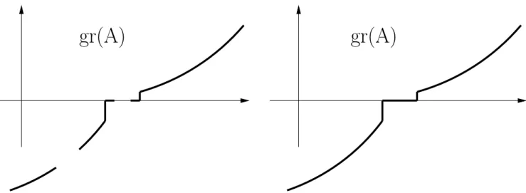
gr(A)

.

Figure 2.1: Left: A monotone operator over R which is not maximal. Right: A maximal monotone extension of the monotone operator

element in the inclusion ordering over X × X among graphs of monotone operators (see Fig. 2.1). Equivalently, the monotone operator A is maximal if the following property holds :

∀(x, y) ∈ X2, _∀(x′, y′)_{∈ gr(A), hy − y}′, x_{− x}′_{i ≥ 0} =_⇒ (x, y)_{∈ gr(A).}

This maximality condition implies that gr(A) is a closed subset of X × X. Denote by I the identity operator, and by A−1 _{the inverse of the operator A, deﬁned by the fact that y ∈ A(x) ⇔ x ∈ A}−1_(y).

Using the monotonicity of A, one can check that ∀(x, y), (x′_{, y}′₎_{∈ gr(A), ∀γ > 0, kx−x}′_{k ≤ k(x+γy)−}

(x′_{+ γy}′₎_{k. In other words, if A is a monotone operator, then the resolvent operator deﬁned for every}

γ > 0 by Jγ := (I + γA)−1 can be identiﬁed with a 1-Lipschitz continuous function (i.e a contraction).

It is well known that A belongs to the set M (X) of the maximal monotone operators on X if and only if, dom(Jγ) = X ([85]). If dom(A) = X, then A is usc [97]. We also know that when A ∈ M (X), the

closure cl(dom(A)) of dom(A) is convex, and limγ→0Jγ(x) = Πcl(dom(A))(x), where ΠS is the projector

on the closed convex set S. It holds that A(x) is closed and convex for all x ∈ dom(A). We can therefore put A0(x) = ΠA(x)(0), in other words, A0(x) is the minimum norm element of A(x). Of importance is

the so called Yosida regularization of A for γ > 0, deﬁned as the single-valued operator Aγ = (I− Jγ)/γ.

This is a 1/γ-Lipschitz operator on X that satisﬁes Aγ(x) → A0(x) and kAγ(x)k ↑ kA0(x)k for all

x∈ dom(A). One can also check that Aγ(x)∈ A(Jγ(x)) for all x∈ X.

A typical maximal monotone operator is the subdiﬀerential ∂f of a function f ∈ Γ0(X), the set of

proper, convex, and lower semicontinuous (lsc) functions on X. In this case, the resolvent (I + γ∂f)−1

for γ > 0 is the proximity operator of γf. The Yosida regularization of ∂f for γ > 0 coincides with the gradient of the so called Moreau’s envelope fγ(x) := minyf (y) +ky − xk2/(2γ) of f .

2.2.2 Differential Inclusions (DI)

We now turn to the diﬀerential inclusions induced by operators. First consider a set valued mapping H: X ⇒ X and a_{∈ X, a solution to the Diﬀerential Inclusion (DI) ˙x(t) ∈ H(x(t)) on R}+ starting at a is

an absolutely continuous mapping x : R+ → X such that x(0) = a, and ˙x(t) ∈ H(x(t)), where ˙x denotes

(23)

such that for every a ∈ X, Φ(a) is the set of solutions to the DI starting at a. We refer to Φ as the evolution system induced by H. For every subset S ⊂ X, we deﬁne Φ(S) =Sx∈SΦ(x).

In the case where H is usc with nonempty compact convex values and satisﬁes the linear growth condition

∃c > 0, ∀x ∈ X, sup{kyk : y ∈ H(x)} ≤ c(1 + kxk) , (2.1) then, dom(Φ) = X, see e.g. [6], and moreover, Φ(X) is closed in the space C(R+, X) endowed with the

topology of uniform convergence over compact sets of R+.

Assume from now on that H = −A ∈ M (X). Then for every a ∈ dom(A), Φ(a) contains exactly one function, still denoted Φ(a) [36]. Note that in the case where A = ∇F, F ∈ Γ0(X), the DI boils

down to the so-called gradient ﬂow. In the sequel, we denote Φ(a, t) = Φ(a)(t). For every t ≥ 0, the map Φ(·, t) : dom(A) → dom(A) is a contraction and can be uniquely extended to a contraction from cl(dom(A)) to cl(dom(A)). Denoting Φ(·, t) this extension, Φ becomes a semiﬂow on cl(dom(A)) × R+,

being a continuous cl(dom(A)) × R+ → cl(dom(A)) function satisfying

Φ(·, 0) = I and Φ(x, t + s) = Φ(Φ(x, s), t) (2.2) for each x ∈ cl(dom(A)), and t, s ≥ 0.

The set of zeros Z(A) := {x ∈ dom(A) : 0 ∈ A(x)} of A is a closed convex set which coincides with the set of equilibrium points {x ∈ cl(dom(A)) : ∀t ≥ 0, Φ(x, t) = x} of Φ. The trajectories Φ(x, ·) of the semiﬂow do not necessarily converge to Z(A). A counterexample is given by the linear maximal monotone operator A deﬁned on R2 _{by A(y, z) = (z, −y) whose set of zeros is Z(A) = (0, 0). The DI}

associated to A boils down to a linear diﬀerential equation in R2_{, (˙y(t), ˙z(t)) = (−z(t), y(t)) for every}

t _{≥ 0. To solve this equation, consider i ∈ C and denote x(t) = y(t) + iz(t) ∈ C. The DI is equivalent} to ˙x(t) = ix(t) whose solutions can be written x(t) = a exp(it), a ∈ C. Finally, x does not converge to zero as t → +∞ in general. However, the ergodic theorem for the semiﬂows generated by the elements of M (X) states that if Z(A) 6= ∅, then for each x ∈ cl(dom(A)), the averaged function

Φ : cl(dom(A))× R+ −→ cl(dom(A))

(x, t) _7−→ 1 t

Z t

0 Φ(x, s) ds

(with Φ(·, 0) = Φ(·, 0)), converges to an element of Z(A) as t → ∞. The convergence of the trajectories of the semiﬂow itself to an element of Z(A) is ensured when A is demipositive [38]. An operator A_{∈ M (X) is said demipositive if there exists w ∈ Z(A) such that for every sequence ((u}_n, vn)∈ gr(A))

such that (un) converges to u, and such that (vn) is bounded,

hun− w, vni −−−→

n→∞ 0 ⇒ u∈ Z(A).

Under this condition and if Z(A) 6= ∅, then for all x ∈ cl(dom(A)), Φ(x, t) converges as t → ∞ to an element of Z(A).

2.3 Random monotone operators

A sequence of elements (An)n∈N in M (X) is said to converge to an element A ∈ M (X) if for every

γ > 0, x _{∈ X, (I + γA}n)−1(x)→ (I + γA)−1(x) as n → +∞. Endowed with this topology, M (X) is

a Polish space [4]. Moreover, the subset of all subdiﬀerentials over X is closed. A random monotone operator is deﬁned to be a random variable A from a probability space (Ξ, G , µ) to (M (X), B(M (X))).

(24)

Let F : Ξ ⇒ X be a set valued function such that F (s) is a closed set for each s ∈ Ξ. The function F is said measurable if {s : F (s) ∩ H 6= ∅} ∈ G for any set H ∈ B(X). An equivalent deﬁnition for the mesurability of F requires that the domain dom(F ) := {s ∈ Ξ : F (s) 6= ∅} of F belongs to G , and that there exists a sequence of measurable functions ϕn : dom(F ) → X such that F (s) = cl {ϕn(s)}n

for all s ∈ dom(F ) [40, Chap. 3][65]. These functions are called measurable selections of F . Consider a function A : (Ξ, G , µ) → (M (X), B(M (X))). For every s ∈ Ξ, γ > 0, x ∈ X, (I + γA(s))−1_{(x) is}

denoted Jγ(s, x). There is equivalence between [4]

1. A is a random monotone operator

2. s 7→ gr(A(s)) is measurable as a closed set-valued Ξ ⇒ X × X function

3. For every γ > 0, x ∈ X, the function s 7→ Jγ(s, x) from (Ξ, G ) to (X, B(X)) is measurable.

Example 2 _{(Random subdiﬀerential). Consider a function g : Ξ × X → (−∞, ∞]. The function g is} said a convex normal integrand [125] if g(s, ·) is convex, and if the set-valued mapping s 7→ epi g(s, ·) is closed-valued and measurable, where epi is the epigraph of a function. Then, the function s 7→ ∂g(s, ·) is an example of random monotone operator [4].

Assume now that F : Ξ ⇒ X is measurable and that µ(dom(F )) = 1. Consider the set Sp

F :={ϕ ∈ Lp(Ξ, G , µ; X) : ϕ(s) ∈ F (s) µ − a.e.} . (2.3)

of Lp _{integrable selection of F . If S}1

F 6= ∅, the function F is said integrable. The selection integral [86]

of F is the set Z F dµ := cl ßZ Ξϕdµ : ϕ∈ S 1 F ™ . (2.4)

For a random monotone operator A : Ξ → M (X), since Jγ(s, x) is measurable in s and continuous in

x (being non expansive), Jγ : Ξ× X → X is G ⊗ B(X)/B(X) measurable by Carathéodory’s theorem.

Denoting Aγ(s, x) the image of x by the Yosida regularization of the operator A(s), this implies the

measurability of Aγ : Ξ× X → X for every γ > 0. Moreover, denoting by D(s) the domain of A(s),

s _{7→ cl(D(s)) is measurable, which implies that the function s 7→ d(x, D(s)) is measurable for each} x ∈ X. Denoting as A(s, x) the image of x by the operator A(s), the set valued function s 7→ A(s, x) is also measurable. In particular, the function s 7→ A0(s, x) is measurable for each x ∈ X, where

A0(s, x) := ΠA(s,x)(0). The essential intersection D of the domains D(s) is deﬁned as [67]

D := [

G∈G :µ(G)=0

\

s∈Ξ\G

D(s) , (2.5) in other words, x ∈ D ⇔ µ({s : x ∈ D(s)}) = 1. Let us assume that D 6= ∅, and that the set-valued mapping A(·, x) is integrable for each x ∈ D. For all x ∈ D, we can deﬁne

A(x) :=

Z

ΞA(s, x) µ(ds) .

We shall sometimes use the notation A(x) = Eξ(A(ξ, x)) where ξ is a random variable with distribution

µ. One can immediately see that the operator _{A : D ⇒ X so deﬁned is a monotone operator.}

Example 3 _{(Interchange property). Let g : Ξ × X → (−∞, ∞] be a convex normal integrand, and let} G(x) =R g(s, x)µ(ds), where the integral is deﬁned as the sum

Z

{s : g(s,x)∈[0,∞)}g(s, x) µ(ds) +

Z

(25)

and

I(x) =

®

+∞, if µ({s : g(s, x) = ∞}) > 0, 0, otherwise ,

and where the convention (+∞) + (−∞) = +∞ is used. The function G is a lower semi continuous convex function if G(x) > −∞ for all x [125], which we assume. Assume also that G is proper. Note that this implies that g(s, ·) ∈ Γ0(X) for µ-almost all s. We provide conditions under which the selection

integral (set to ∅ for the values of x for which S1

∂g(·,x) =∅)

R

∂g(s, x)µ(ds) boils down to ∂G(x). We shall write that the interchange property holds since in this case,

∂G(x) =

Z

∂g(s, x)µ(ds).

First, this will be the case if R |g(s, x)| µ(ds) < ∞ for all x ∈ X. By [102, page 179], this will also be the case if the following conditions hold: i) the set-valued mapping s 7→ cl dom g(s, ·) is constant µ-a.e., where dom g(s, ·) is the domain of g(s, ·), ii) G(x) < ∞ whenever x ∈ dom g(s, ·) µ-a.e., iii) there exists x0 ∈ X at which G is ﬁnite and continuous. Another case where this interchange is permitted is the

following. Let m be a positive integer, and let C1, . . .Cm be a collection of closed and convex subsets

of X. Let C = ∩m

i=kCk 6= ∅, and assume that the normal cone NC(x) of C at x satisﬁes the identity

N_C(x) = Pm

k=1NCk(x) for each x ∈ X, where the summation is the usual set summation. As is well

known, this identity holds true under a qualiﬁcation condition of the type ∩m

k=1riCk 6= ∅ (see also [11]

for other conditions). Now, assume that Ξ = {1, . . . , m} and that µ is an arbitrary probability measure putting a positive weight on each {k} ⊂ Ξ. Let g(s, x) be the indicator function

g(s, x) = ι_Cs(x) for (s, x)∈ Ξ × X. (2.6)

Then it is obvious that g is a convex normal integrand, G = ι_C, and ∂G(x) = R ∂g(s, x)µ(ds). We can also combine these two types of conditions: let (Σ, T , ν) be a probability space, where T is ν-complete, and let h : Σ × X → (−∞, ∞] be a convex normal integrand satisfying the conditions i)–iii) above. Consider the closed and convex sets C1, . . . ,Cm introduced above, and let α be a probability measure

on the set {0, . . . , m} such that α({k}) > 0 for each k ∈ {0, . . . , m}. Now, set Ξ = Σ × {0, . . . , m}, µ = ν_{⊗ α, and deﬁne g : Ξ × X → (−∞, ∞] as}

g(s, x) =

®

α(0)−1_{h(u, x) if k = 0,}

ι_Ck(x) otherwise,

where s = (u, k) ∈ Σ × {0, . . . , m}. Then it is clear that G(x) = 1 α(0) Z Σh(u, x)ν(du) + ιC(x) , and ∂G(x) = Z ∂g(s, x)µ(ds) = 1 α(0)Eν∂h(·, x) + m X k=1 N_Ck(x) .

(26)

Part I

Stochastic approximation with a

constant step size

(27)

Chapter 3 Constant Step Stochastic

Approximations Involving Differential

Inclusions: Stability, Long-Run

Convergence and Applications

The purpose of this chapter is to study the constant step stochastic approximation framework (1.4) in the case where the underlying Diﬀerential Inclusion is induced by an upper semicontinuous operator, see Sec.1.4. We consider a Markov chain (xn) whose kernel is indexed by a scaling parameter γ > 0, referred

to as the step size. The aim is to analyze the behavior of the Markov chain in the doubly asymptotic regime where n → ∞ then γ → 0. First, under mild assumptions on the so-called drift of the Markov chain, we show that the interpolated process converges narrowly to the solutions of a DI involving an usc set-valued map with closed and convex values. Second, we provide veriﬁable conditions which ensure the stability of the iterates. Third, by putting the above results together, we establish the long run convergence of the iterates (xn) as γ → 0, to the Birkhoﬀ center of the DI. The ergodic behavior of

the iterates is also provided. Our ﬁndings are applied to the problem of nonconvex proximal stochastic optimization and a ﬂuid model of parallel queues.

3.1 Introduction

In this chapter, we consider a Markov chain (xn, n ∈ N) with values in an Euclidean space X. We assume

that the probability transition kernel Pγ is indexed by a scaling factor γ, which belongs to some interval

(0, γ0). The aim of the chapter is to analyze the long term behavior of the Markov chain in the regime

where γ is small. The map

gγ(x) :=

Z _y_{− x}

γ Pγ(x, dy) , (3.1) assumed well deﬁned for all x ∈ X, is called the drift or the mean field. The Markov chain admits the representation

xn+1 = xn+ γ gγ(xn) + γ Un+1, (3.2)

where Un+1 is a zero-mean martingale increment noise i.e., the conditional expectation of Un+1 given

the past samples is equal to zero. A case of interest in the chapter is given by iterative models of the form:

(28)

where (ξn, n ∈ N∗) is a sequence of i.i.d random variables indexed by the set N∗ of positive integers

and deﬁned on a probability space Ξ with probability law µ, and {hγ}γ∈(0,γ0) is a family of maps on

Ξ_{× X → X. In this case, the drift g}γ has the form:

gγ(x) =

Z

hγ(s, x) µ(ds) . (3.4)

Our results are as follows.

1. Dynamical behavior. Assume that the drift gγ has the form (3.4). Assume that for µ-almost

all s and for every sequence ((γk, zk)∈ (0, γ0)× X, k ∈ N) converging to (0, z),

hγk(s, zk)→ H(s, z)

where H(s, z) is a subset of X (the Euclidean distance between hγk(s, zk) and the set H(s, z)

tends to zero as k → ∞). Denote by xγ_{(t) the continuous-time stochastic process obtained by a}

piecewise linear interpolation of the sequence xn, where the points xn are spaced by a ﬁxed time

step γ on the positive real axis. As γ → 0, and assuming that H(s, ·) is a proper and upper semicontinuous (usc) (see Sec. 2.2.1) map with closed convex values, we prove that xγ _converges

narrowly (in the topology of uniform convergence on compact sets) to the set of solutions of the diﬀerential inclusion (DI)

˙x(t) _∈

Z

H(s, x(t))µ(ds) , (3.5) where for every x ∈ X,R H(s, x)µ(ds) is the selection integral of H(_{·, x), see Sec.}2.3.

2. Tightness. As the iterates are not a priori supposed to be in a compact subset of X, we investigate the issue of stability. We posit a veriﬁable Pakes-Has’minskii condition on the Markov chain (xn).

The condition ensures that the iterates are stable in the sense that the random occupation measures Λn:= 1 n + 1 n X k=0 δxk (n∈ N)

(where δa stands for the Dirac measure at point a), form a tight family of random variables on

the Polish space of probability measures equipped with the Lévy-Prokhorov distance. The same criterion allows to establish the existence of invariant measures of the kernels Pγ, and the tightness

of the family of all invariant measures, for all γ ∈ (0, γ0). As a consequence of Prokhorov’s

theorem, these invariant measures admit cluster points as γ → 0. Under a Feller assumption on the kernel Pγ, we prove that every such cluster point is an invariant measure for the DI (3.5).

Here, since the ﬂow generated by the DI is in general set-valued, the notion of invariant measure is borrowed from [59].

3. Long-run convergence. Using the above results, we investigate the behavior of the iterates in the asymptotic regime where n → ∞ and, next, γ → 0. Denoting by d(a, B) the distance between a point a ∈ X and a subset B ⊂ X, we prove that for all ε > 0,

lim γ→0lim supn→∞ 1 n + 1 n X k=0 P_(d(x_k_{, BC}_Φ_{) > ε) = 0 ,} (3.6)

(29)

where BC is the Birkhoﬀ center of the ﬂow Φ induced by the DI (3.5), and P stands for the probability. We also characterize the ergodic behavior of these iterates. Setting xn = _n+11 Pnk=0xk,

we prove that

lim

γ→0lim supn→∞

P_(d(x_n_{, co(L}_av_{)) > ε) = 0 ,} (3.7) where co(Lav) is the convex hull of the limit set of the averaged ﬂow associated with (3.5) (see

Sec. 3.4).

4. Applications. We investigate several application scenarios. First, we consider the problem of non-convex stochastic optimization, and analyze the convergence of a constant step size proximal stochastic gradient algorithm. The latter finds application in the optimization of deep neural networks [77]. We show that the interpolated process converges narrowly to a DI, which we characterize. We also provide sufficient conditions allowing to characterize the long-run behavior of the algorithm leading to a convergence proof of the proximal stochastic non-convex gradient algorithm ([98]). Second, we explain that our results apply to the characterization of the fluid limit of a system of parallel queues. The model is introduced in [8, 61]. Whereas the narrow convergence of the interpolated process was studied in [61], less is known about the stability and the long-run convergence of the iterates. We show how our results can be used to address this problem.

Chapter organization. In Sec. 3.2, we introduce the application examples. In Sec. 3.3, we brieﬂy discuss the literature. Sec. 3.4 is devoted to the mathematical background and to the notations. The main results are given in Sec. 3.5. The tightness of the interpolated process as well as its narrow convergence towards the solution set of the DI (Th. 3.5.1) are proven in Sec. 3.6. Turning to the Markov chain characterization, Prop. 3.5.2, who explores the relations between the cluster points of the Markov chains invariant measures and the invariant measures of the ﬂow induced by the DI, is proven in Sec. 3.7. A general result describing the asymptotic behavior of a functional of the iterates with a prescribed growth is provided by Th. 3.5.3, and proven in Sec.3.8. Finally, in Sec.3.9, we show how the results pertaining to the ergodic convergence and to the convergence of the iterates (Th.3.5.4and 3.5.5

respectively) can be deduced from Th. 3.5.3. Finally, Sec. 3.10 is devoted to the application examples. We prove that our hypotheses are satisﬁed.

3.2 Examples

Example 4. Non-convex stochastic optimization. Consider the problem

minimize Eξ(ℓ(ξ, x)) + r(x) w.r.t x∈ X, (3.8)

where ℓ(ξ, ·) is a (possibly non-convex) diﬀerentiable function on X → R indexed by a random variable (r.v.) ξ, Eξ represents the expectation w.r.t. ξ, and r : X → R is a convex function. The problem

typically arises in deep neural networks [129, 115]. In the latter case, x represents the collection of weights of the network, ξ represents a random training example of the database, and ℓ(ξ, x) is a risk function which quantiﬁes the inadequacy between the sample response and the network response. Here, r(x) is a regularization term which prevents the occurence of undesired solutions. A typical regularizer used in machine learning is the ℓ1-norm kxk1 that promotes sparsity or generalizations like kDxk1, where

Random monotone operators and application to stochastic optimization

HAL Id: tel-01960496

https://pastel.archives-ouvertes.fr/tel-01960496

Random monotone operators and application to

stochastic optimization

Adil Salim

To cite this version:

NNT

:

2018SA

CL

T021

Op ´erateurs monotones al ´eatoires

et application `a l’optimisation

stochastique

A

DIL

S

ALIM

Remerciements

Contents

I

Stochastic approximation with a constant step size

24

II

Applications using vanishing step sizes

88

Chapter 1

Introduction

1.1

Theoretical context : Stochastic Approximation

1.1.1

Robbins-Monro algorithm

1.1.2

A general framework

1.2

Motivations

1.2.1

Stochastic Proximal Point algorithm

1.2.2

Stochastic Proximal Gradient algorithm

1.2.3

Stochastic Douglas Rachford algorithm

1.2.4

Monotone operators and Stochastic Forward Backward algorithm

1.2.5

Fluid limit of parallel queues

1.3

Dynamics of Robbins-Monro algorithm

1.3.1

Known facts related with dynamical systems

γ

xa,γ(t)

1.3.2

Convergence of stochastic processes

1.3.3

Stability result

1.4

From ODE to Differential Inclusions

1.5

Contributions

1.5.1

Convergence analysis with a constant step size

γn

x(t)

1.5.2

Applicative contexts using decreasing step sizes

1.6

Outline of the Thesis

Chapter 2

Preliminaries

2.1

General notations

2.2

Set valued mappings and monotone operators

2.2.1

Basic facts on set valued mappings

gr(A)

gr(A)

2.2.2