Granular and particle-laden flows: from laboratory experiments to field observations

HAL Id: hal-01481019

https://hal-univ-rennes1.archives-ouvertes.fr/hal-01481019

HAL is a multi-disciplinary open access archive for the deposit and dissemination of sci-entific research documents, whether they are pub-lished or not. The documents may come from teaching and research institutions in France or abroad, or from public or private research centers.

L’archive ouverte pluridisciplinaire HAL, est destinée au dépôt et à la diffusion de documents scientifiques de niveau recherche, publiés ou non, émanant des établissements d’enseignement et de recherche français ou étrangers, des laboratoires publics ou privés.

Granular and particle-laden flows: from laboratory

experiments to field observations

Renaud Delannay, Alexandre Valance, Anne Mangeney, Olivier Roche,

Patrick Richard

To cite this version:

Renaud Delannay, Alexandre Valance, Anne Mangeney, Olivier Roche, Patrick Richard. Granular and particle-laden flows: from laboratory experiments to field observations. Journal of Physics D: Applied Physics, IOP Publishing, 2017, 50 (5), pp.40. �10.1088/1361-6463/50/5/053001�. �hal-01481019�

Granular and particle-laden flows: from laboratory

experiments to field observations

R Delannay1, A Valance1, A Mangeney2,3, O Roche4, P Richard5 1

Institut de Physique de Rennes, UMR CNRS 6251, Université de Rennes 1, Campus de Beaulieu Bâtiment 11A, 263 av. Général Leclerc, 35042 Rennes CEDEX, France

2

Université Paris Diderot, Sorbonne Paris Cité, Institut de Physique du Globe de Paris, Seismology group, 1 rue Jussieu, 75005 Paris, France

3

ANGE Team, CEREMA, INRIA, Lab. J. Louis Lions, Paris, France

4

Laboratoire Magma et Volcans, Université Blaise Pascal-CNRS-IRD, OPGC, Campus Universitaire les Cézeaux, 6 avenue Blaise Pascal, 63178 Aubière, France

France

5

LUNAM Université, IFSTTAR, MAST, GPEM, site de Nantes, Route de Bouaye, 44344 Bouguenais cedex, France

E-mail: [email protected]

Abstract

This review article provides an overview of dry granular flows and particle fluid mixtures, including experimental and numerical modeling at the laboratory scale, large scale hydrodynamics approaches and field observations. Over the past ten years, the theoretical and numerical approaches have made such significant progress that they are capable of providing qualitative and quantitative estimates of particle concentration and particle velocity profiles in steady and fully developed particulate flows. The next step which is currently developed is the extension of these approaches to unsteady and inhomogeneous flow configurations relevant to most of geophysical flows. We also emphasize that the up-scaling from laboratory experiments to large scale geophysical flows still poses some theoretical physical challenges. For example, the reduction of the dissipation that is responsible for the unexpected long run-out of large scale granular avalanches is not observed at the laboratory scale and its physical origin is still a matter of debate. However, we believe that the theoretical approaches have reached a mature state and that it is now reasonable to tackle complex particulate flows that incorporate more and more degrees of complexity of natural flows.

1. Introduction

Geophysical granular and particle laden flows are common phenomena at the surface of the Earth and other planets (Figures 1 and 2). They consist of solid-fluid mixtures driven by gravity and that propagate in an ambient fluid (except on some extraterrestrial planets) over generally complex topographies. Investigating these phenomena is important because they play a significant role in the global sediment cycle and contribute to shape the landscape. Furthermore, gravitational flows and natural phenomena they can generate, such as tsunamis for instance (Kawamura et al. (2014)), represent severe natural hazards for the populations and infrastructures. Determination of their occurrence and magnitude can also help inferring major climate changes as well as the characteristics of triggering mechanisms. Indeed, gravitational flows are closely related to climatic, volcanic, and seismic activity and thus represent proxies for the time change of these activities (Calder et al. (2002), Hibert et al. (2011, 2014a), DeRoin and McNutt (2012)). This is also of paramount importance to infer

the current or past presence of water on planets such as Mars (Mangold et al. (2010)). Their study is of economic interest as accumulation of deposits in submarine environments may form large hydrocarbon reservoirs while submarine landslides may destroy sea bed infrastructures such as transoceanic communication cables.

Table 1. Main types of geophysical flows and typical ranges of values of most relevant parameters. Flow type setting,

ambient fluid interstitial fluid particle size (m) particle density (kg m-3) particle volume fraction volume (m3) velocity (m s-1) thickness (m) runout distance (km) Subaerial landslides, rockfalls, rock or debris avalanches subaerial, extraterrestrial (a) air, none, small water content 10-3-101 ~2000-3000 ~0.4-0.7 100-1010 109-1013 (a) 10-1-102 10-1-102 100-101 101-102 Submarine landslides subaqueous water - - - 100-1013 - 10-1-102 101- 102 Turbidity currents subaqueous water 10-4-10-1 ~1500-2500 ~0.001-0.1 106-1010 100-101 101-102 101- 103 Snow avalanches (dense (b), powder (c))

subaerial air (water) 10-4-10-1

~100-1000 ~0.1-0.4 (b) ~0.001-0.01 (c) 104-106 101-102 100-101 10-1-100 Pyroclastic density currents (dense (d), dilute (e)) subaerial, subaqueous, extraterrestrial volcanic gases, air 10-6-100 ~500-3000 ~0.1-0.5 (d) ~0.001-0.01 (e) 104-108 100-101 (d) 101-102 (e) 100-102 100-102 Debris flows, lahars subaerial, extraterrestrial water 10-4-100 ~2000-3000 ~0.2-0.8 104-109 100-101 100-101 100-102 a-e

See corresponding values of parameters.

Table 1 presents the main types of geophysical flows and gives ranges of values of the most relevant parameters (see some examples in Figures 1 and 2). The broad terminology associated with these flows reflects their great variety in terms of nature, triggering mechanisms, environments, temporal and spatial scales, and associated mechanical behavior (e. g. Coussot and Meunier (1996), Hungr et al. (2001, 2013)). We focus in this paper on the propagation phase while the study of the initiation phase is a crucial problem at the heart of hazard assessment studies that would require a paper in itself. The terminology considered here is that commonly used in literature based on the nature of the material involved, on the modes of flow generation and on dynamical aspects, but the meaning of the terms may differ between different geophysical communities. Some basic information is given here as a guide for the reader because the different types of flows will be referred to hereafter. Subaerial landslides, rock or debris avalanches are generated by the gravitational destabilization of cliffs, mountain slopes, and volcanic edifices. Rockfalls, rock or debris avalanches are dense granular flows for which the interstitial air or water, if present, is assumed to have a negligible influence on the dynamics (Hsü (1975), Hayashi and Self (1992)), while the term landslide may be used for dense granular flows partially filled or not with water. On Earth, these flows can be very small (rockfalls) but may also have volumes up to ~109 m3 and may contain ice from glaciers at high elevation and/or latitudes (Huggel et al. (2008), Favreau et al. (2010), Moretti et al. (2012)). Extraterrestrial events such as those on the planet Mars may also be very small (Mangold et al. (2010), Johnsson et al. (2014)) or reach huge volumes of up to ~1013 m3 (McEwen (1989), Lucas et al. (2011, 2014)). In submarine

environments, landslides initiate on continental margins or on oceanic ridges, are assumed to be more or less coherent solid masses, and may be more voluminous than their subaerial equivalents (Hampton et al. (1996), Masson et al. (2006)). While submarine landslide activity is rarely observed, recent high resolution surveys of underwater depth of ocean floors reveals small to large landslide deposits that shape the morphology of medio-oceanic ridges (Cannat et al. (2013)). In contrast, turbidity currents are generally smaller flows with low particle volume fraction (Normack et al. (1993), Meiburg and Kneller (2010), Cantero et al. (2012)). Snow avalanches can be dry or wet and the distinction is made between dense slab avalanches, of moderate thickness and high particle concentration, and powder snow avalanches of larger thickness and much lower particle concentration (Hopfinger (1983), Ancey (2001), Schweizer et al. (2003)). Volcanoes generate hot mixtures of volcanic gas and particles, called pyroclastic density currents, through lateral explosion of a magma body or the gravitational collapse of a lava dome or of an eruptive column (Druitt (1998), Branney and Kokelaar (2002), Roche et al. (2013a), Dufek (2016)). Pyroclastic flows and surges represent the dense and dilute end-members of mechanisms, respectively, and often coexist as a dense underflow is commonly overridden by a dilute turbulent ash cloud. Debris flows are dense mixtures of water and solid particles generated in various subaerial environments on Earth and on other planets (Iverson (1997), Iverson et al. (1997), Zanuttigh and Lamberti (2007), Mangold et al. (2010)) and they can derive from landslides (Scott et al. 2001). Lahars are debris flows resulting from the mixing of pyroclastic material with water during subglacial volcanic eruptions or remobilization of pyroclastic deposits by rains (Doyle et al. (2011), Lube et al. (2012)).

Geophysical flows can incorporate their ambient (i.e. surrounding) fluid and/or the substrate on which they propagate. Entrainment of the ambient fluid into a turbulent flow, in both aerial and subaqueous settings, decreases the particle concentration (along with sedimentation) and increases the flow thickness (Hallworth et al. (1993)). It occurs preferentially when the bulk density of the flow is close to that of the ambient fluid, which favors the growth of instabilities at the flow-ambient interface. Hence, fluid entrainment may be particularly efficient in turbidity currents, powder snow avalanches, and dilute pyroclastic density currents (Sparks et al. (1993)). In the latter case, heating and thermal expansion of the entrained air can render the flow buoyant, which leads to spectacular ascending plumes (Woods and Wohletz (1991)).

Geophysical flows such as turbidity currents, snow avalanches, and pyroclastic density currents often have a downward increasing concentration in particles as they consist in a relatively dense basal layer and a more dilute upper layer (Valentine (1987), Nishimura and Ito (1997), Gladstone and Sparks (2002)). The nature of the gradient (gradual or sharp) and the degree of interaction between the two layers are poorly understood. The particles in the currents are often of different natures (rock, pumice, sand, ice, etc.) and shapes. This is likely to affect their coefficients of friction and elastic restitution, for instance, which may in turn affect the flow behaviour and the morphology of the deposit (Goujon et al. (2007), Schneider et al. (2011)). They can also have different densities, typically in the range ~1000-3000 kg m-3. An important characteristic of many geophysical flows is that their grain size range commonly spans several orders of magnitude due to the initial composition of the material released and to efficient fragmentation processes (Figure 2a-b). The smallest particles are often micrometric silts, clays, or ashes, whereas the largest blocks can be of metric to decametric size. Strong heterogeneities in particle size are observed in many deposits in the directions normal and parallel to the topography (Weidinger et al. (2014)). Furthermore, the particle volumetric concentration often changes drastically during emplacement. Segregation of the particles according to their size and/or density also modifies the arrangement of the granular network (e.g. Félix and Thomas (2004), Hill and Yohannes (2011), Johnson et al. (2012), Gray and Hutter (1997), Hill and Tan (2014), Hill and Fan (2016)). Note that segregation of large particles toward the top of the flow is commonly called "normal" by physicists (Brazil nut effect) and "reverse" by geophysicists or engineers, which may be a source of confusion in the literature. For instance, in gravity driven shear flows, Savage and Lun (1988) mention kinetic sieving and squeeze expulsion driving grains into an inversely graded configuration for large grains at the top and small grains at the bottom. Segregation, along with grain size range variations due to particle fragmentation and/or aggregation, can significantly change some flow properties such as hydraulic permeability, which plays a key role in the coupling of the granular and fluid phases. Indeed, pore pressure diffusion may be fundamental and its timescale depends essentially both on the flow hydraulic permeability and on the fluid viscosity and compressibility (e.g.

Pierson (1986), Iverson (1997), Major and Iverson (1999), Iverson and Vallance (2001)). For instance, rapid pressure diffusion due to the permeability increase caused by segregation of coarse particles at the front and lateral margins of debris and pyroclastic flows is thought to cause frictional resistance higher than that in the main body (Major and Iverson (1999), Jessop et al. (2012)). The process of pore pressure diffusion when the particle concentration increases with time (i.e. deflating flows) and/or the interstitial fluid is highly compressible (i.e. gas-particle flows) is yet to be well characterized (e.g. Montserrat et al. (2012)). In these cases, some fundamental insights can be gained from laboratory experiments (e.g. Pailha et al. (2008), Pailha and Pouliquen (2009), Roche (2012), Kaitna et al. (2014), Valverde and Soria-Hoyo (2015)).

Interaction of the flows with their underlying substrate is evidenced by impact marks and scoured surfaces (Sparks et al. (1997), Calder et al. (2000), Pittari and Cas (2004), Le Friant et al. (2004), Conway et al. (2010), Eggenhuisen et al. (2011)). Geophysical flows can also incorporate underlying substrates made of unconsolidated granular materials that often result from earlier events, which increases the mass of the flowing material (Gauer and Issler (2004), Hungr and Evans (2004), Mangeney et al. (2007b, 2010), Berger et al. (2011), Doyle et al. (2011), Mangeney (2011), Iverson (2012), McCoy et al. (2012), Roche et al. (2013a), Farin et al. (2014), Edwards and Gray (2015)). For instance, the mass of snow avalanches on steep slopes can increase by a factor of four through entrainment (Sovilla et al. (2006)). Features typical of basal frictional heating and melting may be evidence of reduced friction due to lubrification of the contacts between the particles or to increase of pore fluid pressure (Legros et al. (2000), Goren and Aharonov (2007), De Blasio and Elverhøi (2008), Goren et al. (2010), Weidinger et al. (2014), Lucas et al. (2014)).

The high variety of geophysical flows renders the development of a unified understanding and theoretical description of these phenomena very difficult. Besides their diversity, natural flows are fundamentally non-permanent, transient phenomena whose propagation is characterized by three steps (i.e., initiation, propagation, and deposition) that commonly involve different physical processes. Initiation spans from nearly instantaneous release of material to continuous supply that can last up to several minutes. Propagation can be characterized by complex flow dynamics, as shown for instance by long-lived debris flows for which surface waves may develop so that several pulses may arise from a single event (Zanuttigh and Lamberti (2007)), or by complex interaction with the underlying topography (Favreau et al. (2010), Moretti et al. (2015)) and an erodible substrate (Moretti et al. (2012)). Deposition typically does not occur everywhere at the same time due to spatio-temporal variations of the flow properties and/or topographical effects as parts of the material come to halt while others are still moving. This is the case for example in self-channelling flows where static lateral levees develop bordering a mobile flow in a channel, partly due to segregation generating coarse-grained levees (Pouliquen et al. (1997), Félix and Thomas (2004), Mangeney et al. (2007a), Jessop et al. (2012), Johnson et al. (2012), Woodhouse et al. (2012), Kokelaar et al. (2014)).

The propagation and energy dissipation of geophysical granular flows are controlled simultaneously by (i) interactions between the particles (friction and collisions) and with the underlying bed, (ii) interactions between the particles and the interstitial fluid filling the interstices between them, (iii) viscous shear of the interstitial fluid (Iverson (1997)), and (iv) shear with the ambient fluid. The interstitial fluid can be different from the ambient fluid. It is either a liquid or a gas (possibly containing fine particles), which is commonly water or air, so that differences in fluid density and viscosity promote various intensities of stresses. The interstitial fluid phase is particularly critical in the dense regime as interstitial pore fluid pressure may arise and damp particles interactions, especially when the fluid is highly viscous and/or compressible. Note that water possibly incorporated during propagation may transform into vapor due to frictional heating or in case of a hot flow.

The measurement and theoretical description of these flows and of the physical processes involved in a natural environment are still open and extremely challenging problems for earth scientists, giving rise to equally challenging physical issues. Table 2 highlights key questions related to these phenomena in the domain of physics and geophysics. This somehow arbitrary separation between physical and geophysical aspects reflects the extreme complexity and variety of the natural flows as well as the difficulty to relate field observation to simple physical experiments and theoretical description. In other words the relevance of using small-scale experiments to model natural flows is questionable. Most of the physical studies on granular flows consider significant simplifications regarding the material properties and the boundary conditions. They commonly involve unidirectional

flows of spherical particles on inclined planes of a length of a few meters (see section 3). The grain size range is often slightly polydisperse and the flow underlying boundary is either flat or covered with glued beads while the influence of lateral walls is often ignored. Even in these very simple systems, a description of the flow in term of rheology, energy dissipation mechanisms, jamming, and flow regime transitions remains essentially incomplete. Field observations by geologists and geophysicists or simple granular flow experiments or models by physicists both provide an extremely simplified view of the natural physical processes at work. One of the major challenges is to make the link between these complementary approaches by taking advantage of the wealth of field data on natural events and of the recent development in the physics of granular flows. Beyond the establishment of constitutive relations that can be used to simulate natural flows, the experimental, theoretical and numerical investigations on simple granular systems may highlight some key processes that guide interpretation of field data.

Table 2: Main questions related to granular geophysical flows, schematically separated into geophysical and physical issues.

Geophysics

How to detect geophysical flows and to assess their related hazards (i.e., flow runout distance, area of deposit, impact pressure on structures, etc.) and indirect impact (tsunamis, etc.)?

What is the contribution of gravitational flows in erosion processes and relief evolution at the surface of the Earth and other planets?

How are gravitational flows related to external forcing (climatic, volcanic, seismic activity)? Could they provide indicators or precursors of these forcing processes?

What physical processes may be at the origin of the high mobility of large natural landslides?

How to quantify and model erosion/deposition processes, solid/fluid interaction, polydispersity and fragmentation at the natural scale?

How to retrieve the mechanisms of propagation and the characteristics of the flows (mass, presence of water, erosion processes, initiation processes, degree of particle-particle and fluid-particle interactions, etc.) from their deposit and/or from the generated seismic or geophysical signal on Earth and on other planets ?

Physics

What is the role played by the interstitial fluid according to the nature of the flow, and conversely, both being coupled? How to describe the grains/fluid coupling, taking into account in particular dilatation/compression effects?

Can we obtain constitutive relations giving a complete description of the granular flows and of their transitions (jammed, dense, dilute)?

How can be captured the boundary conditions and how do they affect the flow? This includes fixed interfaces that are generally associated to an effective friction, and mobile interfaces related to erosion/deposition processes.

How to quantify and describe theoretically the evolution of granular size distribution in space and time (segregation, fragmentation processes) and its coupling with the flow?

Physics and Geophysics

How to measure granular and fluid stresses, particle volume fraction, etc. in both experimental and natural flows?

Figure 1. Example of natural granular gravitational flows. (a) Pyroclastic flows at dawn in January 2014 on

Sinabung volcano, Indonesia. Note the basal hot flow and the upper ash cloud; picture by O. Grunewald. (b) Deposits of the 1993 pyroclastic flows on Lascar volcano, Chile (Jessop et al. (2012)). (c) Hummocky deposits of the 26 km3 Socompa debris avalanche. (d) Erosive debris flows threatening the downslope village of Isafjordur in Iceland ; pictures by A. Mangeney. (e) Ganges Chasma landslide in Valles Marineris on the planet Mars (7º15N; 50º28W) - Image HRSC/DLR/ESA (Lucas et al. (2014)). (f) Gullies on the mega-dune of Russell crater on the planet Mars (5º15N; 12º52E) - Image HiRISE/NASA/JPL-Caltech/Univ. of Arizona (Lucas (2010)).

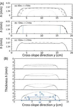
Figure 2. (a) Deposit of the Socompa debris avalanche, Chile, showing the polydispersity of the deposit with

boulders of diameter d larger than 1 m to fine particles of diameter smaller than 10 µm; a zoom within the matrix made of small particles shows a block very well preserved while the block itself and the surrounding matrix are completely pulverized; picture: A. Mangeney. (b) Pyroclastic flow deposit consisting of a matrix of fine ash (size <500 µm) with blocks (>10 cm), Tutupaca volcano, Peru; picture: O. Roche. (c) Front of the 1993 Lascar pyroclastic flow deposits. Morphometry (right) obtained by scanner laser measurements showing the lateral levees surrounding a central channel of lower thickness (Jessop et al. (2012)). (d) Submarine flow deposits on the Mid-oceanic ridge in Krasnov with levee-channel and rounded deposits (Cannat et al. (2013)).

2. Physical Concepts, Theoretical and Numerical modeling

2.1 Forces acting on particles

2.1.1 Particle/particle forces. In dry granular flows, particles interact via contact forces including

collisions and enduring contacts. A collision involving two macroscopic grains is inelastic (in contrast to collision of molecules) and thus dissipates energy. The dissipation is commonly characterized by a coefficient of restitution, e, which is defined as the ratio of the post-collision relative velocity to the pre-collision relative velocity (Louge and Keast (2001)). In dilute granular flows, energy dissipation occurs primarily via dissipative binary collisions. In contrast, in dense granular flows, particles remain in contact within a finite time and dissipate energy via enduring contacts which involve primarily solid friction. Dry solid friction is characterized by a friction coefficient, µ, defined as the ratio of the shear force to the normal force required to initiate sliding, which is material dependent.

2.1.2 Fluid/particle forces. In the presence of an interstitial fluid, particles are subjected to additional

forces. First, a particle undergoes a fluid resistance force which is opposite to its relative motion. This drag force, Fd, can be expressed formally as:

(

)

d Cu u

where up and uf are the velocities of the particle and fluid, respectively. The factor C depends on various parameters such as the particle Reynolds number, the local solid volume fraction φ, etc. For dilute flows of smooth spherical particles, at small particle Reynolds number, the fluid drag reduces to the Stokes force (C=3πdη_f, where ηf is the fluid dynamic viscosity and d the grain diameter), while at high Reynolds particle number, the drag is independent of the fluid viscosity and scales quadratically with the relative particle velocity (C≈0.5

( )

(

)

Second, when two particles come close to each other, they may undergo a repulsive force known as lubrication force. This force arises from hydrodynamic pressure in the interstitial fluid being squeezed out from the space between two particles and is expressed as:

(

)

F_L ≈ 3π 2η_fδ _p (2.2)

where h is the gap between the particles and δup their relative approaching velocity. As a consequence, the interparticle contact forces may be drastically altered in the presence of an interstitial fluid. Gondret et al. (2002) showed experimentally that the dissipation in a binary collision of particles immersed in a fluid is increased in comparison with the dry case and can be expressed in terms of an effective restitution coefficient eeff which follows a master curve depending solely of the Stokes number St= ρpδup d/ηf where ρp is the particle mass density. At small Stokes number (i.e. St < 10) the ratio eeff /edry drops to zero, it approaches 1 at high Stokes number (St > 104) and, on a relatively large interval, eeff can be approximated by (Yang and Hunt (2006)):

St e e

e_eff ≈ _dry−62(1+ _dry)/ (2.3)

If the interstitial fluid is the air, lubrication force can be safely neglected for millimeter particle size, whereas in a liquid, the latter may play a significant role.

Third, particles may be sensitive to the turbulent fluctuations of the fluid flow. This is the case for fine particles in a turbulent fluid flow. The associated transport is called “turbulent suspension”. The dimensionless number for determining whether turbulent suspension is effective or not is the Rouse number:Rouse=w_p/ uκ _*. It is a ratio between the particle fall velocity wp and the vertical fluctuating grain velocity as a product of the von Karman constant κ and the shear velocity u*. Rouse number

smaller than unity indicates that turbulent suspension is effective.

2.2 Flow classification and dimensionless numbers

Among granular flows and particle liquid mixtures, three major categories of flows can be identified according to their solid fraction (the typical values given here correspond to spherical monosized particles): very dilute (φ < 0.01), dilute (0.1 < φ < 0.5) and dense flows (0.5 < φ < 0.59). For very dilute flows, particle/particle interactions play a minor role. These flows include dilute turbidity currents, powder snow avalanches and pyroclastic currents. The motion of particles is driven by the turbulent liquid flow and gravity forces. On the contrary, for dilute and dense flows, particle/particle interactions play an important role. These flows include aerial rock and debris avalanches, landslides, submarine avalanches, debris flows and dense pyroclastic currents. Dense flows can be divided into three subcategories depending on the nature of the particle/particle interactions: (i) particle inertia-dominated regime, (ii) viscous inertia-dominated regime and (iii) fluid inertial resistance-dominated regime. This classification is based on the analysis of the time scale of the particle displacement (see Courrech du Pont et al. (2003a) and Cassar et al. (2005) for further details).

For these different regimes, we can introduce a dimensionless ratio I defined as the ratio of the characteristic particle time scale to the characteristic time equal to the inverse of the flow shear rate

γ

- Particle inertia-dominated regime (i):

I

=

I

=

ρ 

γ

d

P

- Viscous resistance-dominated regime (ii):

p f v P I I= =η γ

- Fluid inertia-dominated regime (iii): p 2 2 f fi

d

P

I

I

=

=

ρ 

γ

Pp is the confining pressure, ρp and ρf are the particle and fluid density respectively. Note that we drop the numerical factor in the definition of I to make it consistent with the usual definition of inertial number (see Eq. (2.10)). The inertial regime (or Bagnoldian regime) has raised a great interest in the granular physics community and various theoretical approaches have been developed to model this flow regime. Two emblematic approaches are the granular kinetic theory for collisional granular flows and the so called “µ(I)” rheology for dense granular flows.

Alternative dimensionless numbers have been introduced in the literature (Iverson (1997)) on the basis of the comparison of particle and fluid stresses. One can mention the Savage and Bagnold number defined respectively as the ratio of the inertial grain shear stress to the weight of flowing layer per unit surface

(

)

and the ratio of inertial grain shear stress to viscous shear stress,

(

)

where H is the thickness of granular layer. The Savage number NSav is nothing but the square of the inertial number Ipi in which the confining pressure is driven by the hydrostatic force (Pp ∼ (ρp -ρf)gH ). The Bagnold number is a simple combination of Ipi and Iv: NBag ∼ Ipi2

/Iv. High Bagnold number thus refers to particle inertia-dominated regime.

2.3 Dry granular flows

We focus here on the inertial regime, where the stress due to the grains is far larger than that exerted by the fluid, so that one may ignore the effects of the ambient fluid and consider inter-particle interactions only.

2.3.1 Collisional Granular flows: kinetic theory. In rapid granular flows, the grains interact mainly through binary collisions in a way that is reminiscent of molecules interacting in a gas. There are nevertheless significant differences between a “granular gas” and a molecular gas. The disparity of sizes between grains and molecules is not the direct cause of these differences. The fact that grain collisions are not elastic, and thus dissipative, has major implications concerning the behaviour of grain assemblies: granular gases are always in non-equilibrium states.

It is common to define the granular temperature in a slightly different way than for molecular gases: T is defined as the average (over volumes and time ranges) of the square of the grain velocity fluctuations. This statistical definition does not need to refer to a state of equilibrium. One of the main applications of the concept of granular temperature is the construction of kinetic theories. The term “kinetic theory” is often used in different contexts. The more general one is a mesoscopic approach where the state of the system is described using the distribution function specifying the distribution of particle positions and velocities. In most cases, it cannot be solved exactly. The other one, called Chapman-Enskog expansion, is an approximation where the two particle distribution function is expressed as the product of the single particle velocity distribution functions, and the pair distribution at contact. This approach neglects the correlations. The hydrodynamic equations of motion resulting from the application of these theories resemble the compressible Navier–Stokes equations:

( )

(

)

∂

ρ

φ

ρ

φ

(

)

φ

ρ

Here, φ is the volume fraction, u the mean velocity, σ the stress tensor and f the body force density. The equation for the energy density, e, contains a sink term Γd that represents the loss of energy due to

the inelasticity of the collisions (q is the energy flux vector):

(

)

pφ ∂e ∂t+u⋅∇e =−∇⋅q+σ:∇u−Γ

ρ (2.8)

This term is responsible for the existence of many phenomena that characterize granular gases. The hydrodynamic description is completed by constitutive relations expressing σ, q and Γd in terms of

the hydrodynamic fields. Kinetic theory provides local constitutive relations through the application of the Chapman-Enskog expansion. The constitutive relation for τ is expressed as in a Newtonian fluid:

(

)

[

]

[

(

( )

)

]

p u1 u u

σ= − + λ−2η 3∇⋅ +η ∇ + ∇ (2.9)

The energy flux vector q=−κ∇⋅T, the pressure p = ρpφ(1 + 4φg12)T, the viscosities λ and η, the conductivity κ and the sink term Γdare given in terms of the volume fraction, the granular temperature

T = 2e/3 and the pair distribution at contact g12(φ) (Jenkins and Savage (1983), see also Delannay et al. (2007) and references herein).

The solutions of these equations have had some success in describing relatively dilute flows or moderately dense flows in the absence of gravity (Azanza et al. (1999), Forterre and Pouliquen (2001), Xu et al. (2003)).

In the dense limit, this approximation generally fails. An improvement of the models to incorporate the effect of correlations is necessary to describe the dense flow regime. The challenges for applying such ab initio theories for dense granular flows are discussed in Delannay et al. (2007) and Kumaran (2015).

2.3.2 Dense granular flows. In the dense flow regime, collisions still exist, but they can involve more

than two bodies and become so frequent that very strong energy dissipation occurs (inelastic collapse). Contacts between particles tend to be enduring and long-lasting; the contact network can percolate through particles. The enduring frictional contacts induce correlations between the velocities and/or locations of the particles.

There have been several attempts to extend the simple kinetic theory to include higher volume fractions, greater dissipation in collisions, and multiple or enduring contacts. The existing constitutive relations of the kinetic theory need to be modified by the incorporation of the correlations associated with the enduring and/or repeated contacts. However, the appropriate form of this modification has yet to be determined. Up to now no constitutive equations are available in the dense regime.

Several studies (Da Cruz et al. (2005), GDR MiDi (2004)) have pointed out that simple dimensional arguments could provide an interesting framework for constitutive laws for dense granular flows. These may be phrased as empirical constitutive relations for the shear stress and normal stress in steady homogeneous shearing. An assembly of rigid frictional spheres of diameter d and mass density ρp, confined under a normal stress P in between two bumpy planes, is sheared at a given shear rate

γ

( )

I

I

d

P

P

µ

γ

ρ

The form of the function µ(I) can be obtained from the numerical simulations of plane shear (Da Cruz et al. (2005)) or indirectly by experimental measurements for flow down inclined planes (cf. section 3.2). The function µ(I) goes from a minimum value µs for very low I (quasi-static regime) up to an asymptotical finite value µ2 when I increases. It can be expressed by the following expression (Jop et

al. (2005)):

( )

(

) (

)

µ (2.11)

where I0 is a constant. The values of coefficients are material-dependent, for instance typical values for glass bead are µs = tan(21°), µ2 = tan(33°) and I0 = 0.28 (GDR Midi (2004), Jop et al. (2005)).

Another relation, also derived from dimensional analysis, gives the variation of the volume fraction; φ is, in general, an affine decreasing function of I (Da Cruz et al. (2005)). This relation completes the constitutive laws:

(

)

max φ φ

φ

φ= − − (2.12)

Typical values are φmax = 0.6 and φmin = 0.5 (Pouliquen et al. (2005)). The latter equation is only for I lower that 1, i.e. for volume fraction larger than φmin.

Ageneralization of this approach to tensorial constitutive relations for incompressible 3D flows has been proposed (Jop et al. (2006)):

τ I σ= P− + , with τ=ηγ, and

( )

P represents an isotropic pressure, by definition it is the negative one-third the trace of the stress tensor, and τ is the deviatoric component. The effective viscosity η is a function of the second invariant

γ

This relation can be extended for the compressible case by replacing the strain rate tensor by its deviatoric component in (2.13) (Cortet et al. (2009), Börzsönyi et al. (2009)). It implies, in addition, a univocal dependence of the volume fraction on the inertial number.

Considering (2.13), in the limit of a shear rate going to zero, one can see that the material flows only if the following Drucker-Prager-like yield criterion is satisfied: ||τ|| > µs P. Below the threshold, the medium behaves locally as a rigid body. Note that the constitutive relation (2.13) can be separated into two terms: a Drucker-Prager yield stress term involving the constant friction coefficient µs, and a viscous term with a viscosity depending on both the pressure and the norm of the strain rate tensor (Ionescu et al. (2015)). The specificity compared to classical Bingham or Herschel-Bulkley fluids is that the yield stress depends on the local pressure and the effective viscosity depends both on the shear rate and on the local pressure.

The µ(I) rheology had some success in reproducing quantitatively experimental observations in relatively simple situations such as granular column collapses (cf. section 3.4.2). Nevertheless, (2.13) contains very strong assertions: stress and strain rate tensors have to be aligned, and the second invariants should satisfy the relation:

( )

τ

(2.14)

where the function µ(I) follows (2.11). The tensorial relation (2.13) has been tested by numerical simulations using DEM (see section 2.7) in different situations (Cortet et al 2009, Börzsönyi et al. (2009)). It turns out that the alignment between stress and strain rate tensors fails. Interestingly, the relation (2.14) works better. But it does not seem to give a friction coefficient law similar to (2.11). A logarithmic decay is observed (Cortet et al. (2009)) for vanishing values of I (leading to very low

values of the friction coefficient) and a non-monotonic variation of µ(I) is reported at larger values of

I (with high value for the friction coefficient) (Börzsönyi et al. (2009)). A granular rheology that

generalises the μ(I) model and incorporates first and second normal stress differences has been

recently proposed (McElwaine et al. (2012)).

Another questionable point is that such a rheology does not use the notion of granular temperature which is at the base of the kinetic theory (Jenkins and Richman (1985)) even in the case of dense flows. The friction function is purely phenomenological without explicit links between the coefficients used and the grain properties. Moreover, the variation of the effective friction µ with the inertial number I - which has been obtained empirically and not theoretically - has been recently questioned (Holyoake and McElwaine (2012)). Clearly, a link between the µ(I)-rheology and the grain-scale physics is still missing. Note also that it has been recently shown (Barker et al. (2015)) that, in the incompressible limit, the µ(I) rheology is only mathematically well-posed for intermediate values of the inertial number. At high and low inertial numbers the equations are ill-posed, i.e. the growth rate of small perturbations increases infinitely fast in the high wavenumber limit. The practical significance of this is that two-dimensional time-dependent simulations in the ill-posed regime will exhibit short wavelength instabilities that will get progressively stronger as the resolution is enhanced, i.e. the results will be grid-dependent. This points out that there is some important missing physics (force chains, effect of grain stiffness) for both high and low inertial numbers where the problem is ill-posed.

The µ(I)-rheology is a local rheology in its current form, it is thus not valid close to the jamming transition (Staron et al. (2010), Deboeuf et al. (2005)), or when non-local effects are not negligible (Nichol et al. (2010), Reddy et al. (2011)). As already mentioned, the enduring frictional contacts induce correlations between the velocities and locations of the particles. These spatial correlations become very important, both in the force network and velocity fluctuations, near the jamming transition. To incorporate these non-local effects in the constitutive relations is not an easy task. It is a generic question emerging in the study of other complex fluids near jamming: foams, emulsions, colloidal suspensions. Some of the attempts to develop non local theories are described in GDR MiDi (2004), Delannay et al. (2007), Henann and Karmin (2013) and Jop (2015). For example, Jenkins (2006, 2007) modified the kinetic theory by introducing a length associated with the size of particle clusters into the expression of the rate of collisional dissipation. This theory has been extended to very dissipative, frictional spheres (Jenkins and Berzi (2010)). The latter theory has the capacity to reproduce, at least qualitatively, experimental results of dense, unconfined, inclined granular flows over a rigid bumpy base and dense, confined flows over an erodible base (cf. section 3.2).

2.4 Modeling particle- fluid mixtures

2.4.1 Introduction. Debris flows, landslides or submarine avalanches are geophysical events

characterized by the flow of a mixture of liquid and particles down a slope. The rheology of this mixture presents significant modeling challenge. We lack a full understanding of how these flows are initiated but there is a growing understanding of processes governing flows, once motion has been triggered.

2.4.2 Single-phase model. Single-phase models have been employed to describe fluid particle mixture.

They are based on a unique rheological relation between the shear stress and the shear strain rate and consider the mixture as a continuum. They typically employ a non-newtonian rheology to incorporate the effect of grain interaction (Takahashi (1991), Coussot (1994), Chen and Ling (1998), Brufau et al. (2000)). The rheologies adopted range from rigid-viscous (yield, followed by a linear viscous stress, Bingham (1922)) to collisional (shear and normal stresses quadratic in the shear rate, Bagnold (1954)). These approaches become inappropriate when the fluid phase and the granular skeleton have a differential motion, inducing gradients of fluid pressure. The relative motion between the fluid and the particle phase can be created by various mechanisms: e. g. the development of hydrostatic pressure gradients or simply the compaction or dilation of the granular network. The last point is well illustrated when the flow is initiated or comes to rest as the solid volume fraction of the granular phase changes. Granular materials are indeed known to change volume when sheared: a dense packing dilates while a loose one compacts (Reynolds (1886)). When the granular material is saturated with a

fluid, the change in volume fraction induces a pore pressure gradient (Iverson et al. (2000)), which in turn either alters the particle motion (dilation) or reduces interparticle friction (compaction).

2.4.3 Two-phase model. More elaborate models distinguish between the two phases and assume that

they interact through drag and buoyancy. These models are referred to as "two-phase" or "two-fluid" models (Anderson and Jackson (1967), Drew (1983), Bedford and Drumheller (1983), Anderson et al. (1995), Jackson (1997, 2000)) and are based on an averaging of mass and momentum balance laws for fluid and solid constituents.

Our purpose here is not to list all the two-phase models of the literature but rather to discuss about the different key assumptions made in these models. For this, we shall first focus on simple flow configurations corresponding to unidirectional, steady and fully developed flows before addressing issues concerning unsteady or inhomogeneous flows.

2.4.4 Steady and fully developed regimes. We consider a unidirectional, steady and fully developed

flow down an incline, consisting of a mixture of granular material and interstitial fluid, each of constant specific mass density ρp and ρf, respectively.

Figure 3. Sketch of a steady and fully developed flow down an incline of angleθ

In this simple flow configuration, the momentum equations take the following forms,

(

)

for the particle phase, and

(

)

(

)

(

)

(

)

for the fluid phase. up and uf stand for the velocities of the solid and fluid constituents, respectively, τxz,p and τxz,f for the particle and fluid shear stress, Pp and Pf for the particle and fluid pressure, and φ

for the solid volume fraction. The factor C which quantifies drag, depends on various parameters (Reynolds number, solid fraction …). The simplest form of the latter factor that incorporates viscous and form drag and concentration dependence reads as (Dallavalle (1943), Richardson and Zaki (1954)):

H z

x θ

(

)

To complete the system equations, closure models for both the fluid and particle shear stress should be supplemented. For turbulent liquid flows, the fluid shear stress can be described by a simple classical turbulent closure based on the mixing length theory (Berzi and Jenkins (2008)) as:

(

) (

)

where νt is the turbulent viscosity modeled by ν_t =l2∂_zu_f. The spatial length l is the mixing length and is proportional to the distance from the flow base (l =κz, where κ is the von Karman constant) for a turbulent liquid flow free of particles. The presence of particles is however expected to influence the turbulence and thus to modify the mixing length. In absence of any experimental data, the simplest approximation is to use the law (2.18). However, more elaborate models have been developed to account for the influence of particles on fluid turbulence (Jenkins and Hanes (1998), Hsu et al. (2003, 2004), Cantero et al. (2012)).

The closure for the particle phase is another crucial issue which is not yet solved. Depending of the flow regime, different closure models have been proposed.

(i) For collisional flows of heavy grains (called sheet flows), where collisional dissipation dominate viscous dissipation (Jenkins and Hanes (1998)), the particle shear stress can be derived from the kinetic theory of granular gas (see section 2.3.1). The particle pressure and the particle viscosity are thus given in terms of the granular temperature. This simple model has the capacity to predict profiles of particle concentration and particle mean velocity in steady and fully developed sheet flows.

(ii) For dense liquid particle mixture, several recent approaches employing the "µ(I)" rheology for the particle shear stress closure (cf. section 2.3.2) have been developed by Cassar et al. (2005). For dense viscous granular suspension, a more refined relation has been proposed by Boyer et al. (2011). According to the flow regime (inertial or viscous), the pertinent inertial parameter to be considered is respectively Ipi and Iv. In this context, Berzi and Jenkins (2008) have considered the problem of steady and fully developed flows of particles and fluid down a slope. They made the assumption that the fluid rheology is described by an eddy viscosity model (cf. (2.18)) and the granular phase by a shear-rate-dependent friction law µ (I). They investigated the case where the particle inertia dominates the fluid drag (i.e., particle inertia-dominated regime). In other words, they assumed that I = Ipi. This approach was shown to be successful for predicting quantitatively the velocity and density profiles observed in the experiments of Armanini et al. (2005) in which a mixture of fluid and particles is recirculated through an inclined channel. This approach is restricted to steady and fully developed flows and therefore disregard dilatancy effects.

For describing bed load transport in laminar flows, Aussilous et al. (2013) have implemented a two-phase continuum model using a shear-rate-dependent friction law µ (Iv) for the granular phase and a volume-fraction-dependent viscosity for the fluid phase. This approach provides reasonable predictions for particle velocity and particle density profiles.

2.4.5 Unsteady flows. We shall now discuss the capability of the two-phase approaches to model the

transient dynamics during which the mixture can contract or dilate.

During the transient, part of the relative vertical displacements between the fluid and the granular phase are caused by the dilation and compaction of the granular material.

These displacements affect the pressure field. The classical approach is to split the fluid pressure into two contributions:P_f =P_fh+P_fe, where P_fh is the hydrostatic fluid pressure, verifying ∇P_fh =ρ_fg and

e f

P is the excess pore-fluid pressure.

The key issue is thus to provide a closure relation between the particle volume fraction and the excess pore pressure. Iverson (1997) argued that it is reasonable to assume that the particle volume fraction is a function of only the excess pore pressure and that the change in particle volume fraction due to changes in excess pore pressure can be expressed in terms of the compressibility coefficient

e f P

K =∂φ ∂ of the sediment-water mixture. Within this hypothesis, the equation for the particle volume fraction reduces to a standard diffusion equation that can readily be solved.

Other closure equations can be found in the literature. For example, Pailha and Pouliquen (2009) consider an equation relating the relative variation of the particle volume fraction to the shear-induced dilatancy angle. More precisely, their model is inspired from the critical state theory proposed by Roux and Radjai (1998) and is based on the concept of the dilatancy angle y, which gives the rate of dilation (compaction) of the material under shear. Based on this theory, the closure equations for the particle shear stress and pressure are modified and rewritten as:

p eq p , p , xy tan P xy τ y τ − = (2.19) K y φ φ₋ eq ₌tan _(2.20) supplemented by γ y φ φ tan  1 = dt d (2.21)

where γ is the local particle shear rate.

τ

2.5 Boundary conditions

The physical principles on which the equations of continuum models are based are the balance laws of mass and momentum (and energy) and constitutive closure equations describing the mechanical behaviour of the material involved. These equations are then used together with boundary conditions to predict the motion of the system.

The behaviour of granular flows contrasts with the one of single phase newtonian fluids as the former depend crucially on the nature of the boundaries (i.e., the properties of the base atop which the flow occurs and the possible presence of lateral confinement). Most experimental and numerical studies generally consider bumpy, flat frictional or erodible basal boundaries. Bumpy boundaries usually consist of particles glued on a flat substrate. In most studies, glued particles are the same as those of the flowing material. However, the bumpiness can be increased or decreased by using grains larger or smaller than the flowing grains. The spatial repartition of the grains can also be used to modify the bumpiness of the boundary.

The conditions at the boundaries, for granular flows, differ from the one used for Newtonian fluids. For the latter, no-slip conditions at solid boundaries is often achieved. In contrast, a granular flow slips relative to a boundary; so, in addition to collisional dissipation at the boundaries, fluctuation energy can be generated by slip (Richman (1988)). Consequently, boundaries can either provide or remove fluctuation energy from the flow.

Establishing ab initio boundary conditions for granular gases is complex: in addition to the difficulty of solving the Boltzmann equation near a solid boundary, one has to know the properties of the collision between the particle and the boundary. The feed-back effect of the boundary on the distribution function of the incoming particles must be taken into account. Approximate boundary conditions at solid surfaces describing the way energy fluctuation is provided to the flow can be applied to flows down bumpy inclined (Richman and Marciniec (1990), Jenkins (1994), Delannay et al. (2007), Kumaran (2015)).

Within the framework of the µ(I) rheology, boundary conditions also cause difficulties. For example, the effect of changing the degree of bumpiness of a bumpy base is not clear: does it only modify the shear and velocity in a boundary layer? Or does it change the whole bulk rheology (Goujon

et al. (2007)). It has been shown that relatively small changes at the boundary can induce transitions from disordered to ordered flow states (Silbert et al. (2002), Kumaran and Maheshwari (2012), Kumaran and Bharathraj (2013)). The slip velocity at the boundary (flat or, to a lesser extent, bumpy) should be related to the physical characteristics of the grains and the boundary (Artoni et al (2009), Artoni et al. (2012)).

Free surface flows induce other questions concerning boundary conditions. Phase transition from liquid to gas may occur at the free surface. As the pressure decreases, the number I becomes very large and the kinetic regime appears. This transition is neither predicted nor described by the µ(I) rheology. Another transition also appears in free conditions: as will be seen in section 3.3, unconfined flows can create lateral levées, which correspond to erodible boundaries. It can be seen as a jamming/unjamming transition. The same behaviour is also observed on very dissipative bases (Louge et al. (2015)), and when there is the spontaneous formation of a heap, called SSH (see section 3.2). The flowing “liquid” zone is in contact with a quasi-static part where the displacement of the grains decreases exponentially. The number I vanishes when approaching this part. The µ(I) rheology does not describe this quasi-static regime, which probably requires a non-local rheology, as already mentioned (section 2.3.2).

In the case of a flow over an erodible base composed of the same material, different approaches have been developed to describe the erosion/deposition process. One of them is the BCRE model (Bouchaud et al. (1994), Boutreux et al. (1998)). Assuming a thin flow on a pile slope close to the angle of repose, this model provides a continuum phenomenological description of the surface dynamics by two variables: b(x,t), the local height of the pile (profile of immobile grains) and h(x,t), the thickness of flowing grains. These variables are dynamically coupled by an interaction term Γ(b,h) allowing conversion from flowing to static grains and vice versa (deposition/erosion). The mass conservation is then expressed as:

Γ + ∂ ∂ = ∂ ∂ + ∂ ∂ Γ − = ∂ ∂ 2 2 x h D x h U t h t b (2.22)

where U is the constant drift downhill velocity of the rolling grains, and D is a constant diffusion coefficient. To close the model, a phenomenological relation between the interaction term Γ and the local slope θ has to be written. A first approach is to set the amplitude of exchange rate with the distance to a neutral inclination angle θn: Γ=

γ

(

θ

θ

)

than a few grain diameters (h > λ) the previous exchange term is not realistic, grains from the upper layers do not interact with the static phase (Boutreux et al. (1998)): Γ=v_up

(

)

(2015) have listed the alternative formulations of the exchange rate term that have been proposed in the literature. We shall point out that this simple phenomenological model can be formally derived from hydrodynamic models based on Saint-Venant equations (e.g., Gray (2001), Aradian et al. (2002), Bouchut et al. (2008)). However, as highlighted in Bouchut et al. (2008), the energy balance of these models is not always consistent. More refined descriptions of erosion and deposition processes can be developed from the knowledge of the constitutive law of the granular fluid coupled with a yield criterion without additional phenomenological law for the erosion rate (Bouchut et al. (2016), Lusso et al. (2015a)). The exchange rate cannot be derived explicitly except in very simple configurations.

For fluid particle mixture continuum models, the same difficulties arise for accounting properly for what happens at the boundaries and for deriving appropriate boundary conditions. Recently, an interesting approach has been introduced by Ancey and Heyman (2014) as a microstructural model of bedload transport, which describes the advection and scattering of coarse particles carried by a turbulent water stream down a sloping granular bed. Fluctuations of the particle flux are generated by particle exchanges with the bed consisting of particle entrainment and deposition. The evolution of the

number of moving particles is described probabilistically using a coupled set of reaction-diffusion master equations.

Another key issue in fluid particle mixture continuum models is to describe what happens at the free surface. In particular it is important to describe different free surfaces for the solid and fluid phases to make it possible for the fluid to be sucked or expelled from the granular material when dilatancy effects are accounted for (Bouchut et al. (2015b)).

2.6 A simplified model: depth averaged approach

Practically, solving the mass and momentum conservation full set of equations requires a prohibitive computational cost when applied to natural flows over real topography and simplifications are necessary.

A first approximation is to assume that the flow is thin compared to its extent along the slope (i. e. small aspect ratio). This is the case for most geophysical flows that are a few meters thick and travel distances of several hundred meters to several kilometers. Asymptotic development of the equations based on this thin-layer approximation makes it possible to neglect some terms such as the vertical acceleration, generally leading to the hydrostatic pressure assumption. Thin layer models solving the resulting simplified 2D or 3D equations have been proposed based on the partial fluidization method that takes into account an order parameter describing the state of the granular matter from static to flowing (Aranson and Tsimring (2002), Mangeney et al. (2007b), Aranson et al. (2008)) or by using visco-plastic models with a yield stress separating static and flowing zones (Bouchut et al. (2016), Lusso et al. (2015a)).

Assuming thin-layer flows together with averaging the equations over the depth of the flow makes it possible to further reduce the computational cost as proposed in the pioneering work of Savage and Hutter (1989) partially based on former german (Voellmy (1955)) and russian (Grigorian et al. (1967)) works on snow avalanches (Figure 4). In that case, the whole granular material is assumed to be flowing. The resulting system (so-called Saint-Venant or shallow-water) involves two unknowns, the thickness and the mean (depth-averaged) velocity of the flowing mass. This hydrodynamic model is widely used to simulate natural flows. The first order asymptotic development leads essentially to a hydrostatic pressure (including centrifugal forces) even though attempts have been made to include the vertical acceleration (Denlinger and Iverson (2004)). The mass and momentum conservation equations in the simplest 1D case (i. e. flow over a 2D topography b(x)) then read

( )

( )

( )

θ

µ

θ

θ

where 𝑢�(𝑋, 𝑡) is the depth-averaged velocity in the downslope direction X (see Figure 4) and |𝑢�| it’s absolute value, ℎ(𝑋, 𝑡) is the flow thickness, 𝜃(𝑋, 𝑡) the slope angle, and 𝑅(𝑋, 𝑡) the curvature radius of the topography. In that case, the momentum equation reduces to the balance between the acceleration, the gravity force, the force related to the pressure gradient and the friction force including centrifugal acceleration effects.

Formally, the friction terms derived from the Coulomb friction law based on this depth-averaged asymptotic method appear both in the basal shear stress and in the pressure gradient term when anisotropy of normal stresses is taken into account (e. g. Gray et al. (1999), Denlinger and Iverson (2004)). However, because accurate development of the thin-layer approximation for a Coulomb friction law has never been done over a 3D arbitrary topography and because anisotropy effects have been questioned for granular flows (e. g. Ertas et al. (2001)), the models generally only consider the term related to the basal shear stress to describe the friction dissipation (e. g. Mangeney-Castelnau et al. (2005)). As a result, these models loose the relative importance of the sliding and shearing contributions to the flow. Consequently, one of the key issues of the method is the modelling of the averaged friction dissipation at the base. The basal friction is generally described phenomenologically

in the framework of Coulomb friction using friction coefficient which may be constant or depend on the inertial number (see for example Pouliquen and Forterre (2002), Mangeney-Castelnau et al. (2003), Mangeney et al. (2007a), Pirulli and Sorbino (2008)). Note, however, that fitting the basal friction dissipation (the only dissipation term in the model) to reproduce deposit extent of laboratory or field scale events result implicitly in an empirical quantification of the whole effective friction within the flow (Lucas et al. (2014)).

Figure 4. 2D depth-averaged thin-layer continuum model where the depth-averaged velocity field ū(x,y,t) and

the flow thickness h(x,y,t) are calculated at time t. Note that the velocity is averaged in the Z-direction, where (X,Y,Z) is the variable reference frame linked to the topography b(x,y) and θ is the steepest slope angle. The curvature of the topography is a tensor and we represent here one of its component Rx (see Appendix A of

Mangeney et al. (2007a)).

One of the main difficulties in deriving thin-layer depth-averaged models is to appropriately take into account topography effects, which is a key issue for application to natural landslides. Indeed, these flows are thin in the direction perpendicular to the flow and not in the vertical direction (Figure 4). For these reasons, a series of asymptotic developments have been performed in a variable reference frame linked to the topography for complicated but specific topographies (see Pudasaini et al. (2007) for a review). By considering a fixed reference frame but applying the thin-layer approximation in the direction perpendicular to the slope, Bouchut et al. (2003) and Bouchut and Westdickenberg (2004) derived a model that takes into account accurately all the curvature terms for flows over an arbitrary topography, including centrifugal forces ignored in other models (see Appendix A of Mangeney et al. (2007a)). These terms can be important in the dynamics of natural landslides (Favreau et al. (2010), Moretti et al. (2015)).

By assuming that the whole material flows, the Savage-Hutter model fails to capture the features of flows for which interaction with an erodible base prevails. This is the case for example for dam-break granular flows (see section 3.4). Indeed the transition between static and flowing regions in a depth-averaged model requires the determination of an equation for the evolution of the moving interface between the flowing and non-flowing parts, an interface that is not always well defined. As discussed in section 2.5, this point is currently a matter of debate, notably because a quantitative study of the erosion/deposition rate at the grain scale is still missing. Moreover, the proposed approaches are generally overly schematic to be extended to natural flows over real topography (Bouchut et al. (2008)). A key new approach using the depth-averaged µ(I)-rheology and prescribed Bagnold velocity profiles (Gray and Edwards (2014)) explicitly model the formation of erosion-deposition waves (Edwards and Gray (2015)), where completely stopped regions can form between mobile wave crests. A depth-integrated model taking into account a linearization of the μ(I)-rheology and prescribed S-shaped velocity profile was also proposed by Capart et al. (2015). This model reproduces granular flows over erodible beds. However, by prescribing a specific shape of the velocity profiles, these models cannot reproduce the different profiles observed in highly transient flows. A new alternative