Can hyperspectral techniques improve estimates of carbon
stocks in agricultural soils?
A. Stevens
a, B. van Wesemael
a, S. Touréb, G. Vandenschrick
aand B. Tychon
b aDepartment of Geography (UCL), place Pasteur 3, 1348 Louvain-la-Neuve, Belgium,
email: stevens@geog.ucl.ac.be
b
Biometeorological Stress Unit (FUL), avenue de Longwy 185, 6700 Arlon, Belgium
ABSTRACT
Soil organic carbon (SOC) represents one of the major pools in the global carbon cycle. However, fluxes of CO2
from soils into the atmosphere by respiration or inversely sequestration of CO2 through photosynthesis and
subsequent immobilisation in the form of humus are difficult to quantify. In principle changes in SOC stock over time reflect CO2 fluxes. The detection of these stock changes, however, require intensive sampling mainly due to
the large spatial variability of SOC both within individual fields and larger units with similar soils and land use. The aim of this paper is to evaluate the potential of airborne-hyperspectral techniques using a CASI sensor and hand held Near Infrared Spectroscopy (NIRS) with an ASD spectrometer to conduct SOC inventories of individual parcels. During a field campaign in the Belgian Ardennes during Octobre 2003, more than 120 sites on a regular grid within 13 freshly ploughed fields were selected. At these sites, field spectra of the bare soil have been measured and samples from the topsoil were taken. SOC content (Walkley and Black), soil moisture and bulk density of these samples have been determined. As a first step, the soil reflectance has been transformed (log (1/R), Savitsky-Golay smoothing and derivative, gap derivative, moving average) in order to filter the spectral responses and to eliminate noise. Then, we used both stepwise and partial least square (PLS) regression analysis to relate these spectra to measured SOC contents. Regression models performed much better when the data were divided in two sub-groups representing different moisture conditions of the soil surface. These statistical model calibrations were validated on an independent data set. Standard Error of Prediction (SEP) ranged from 0.19 to 0.24 % carbon for the field spectra determined using the ASD depending on soil moisture of the surface layer. This is a little bit more than the reproducibility error inherent to the Walkley and Black analysis. Airborne CASI techniques performed less well mainly due to the narrow spectral range. Tests on airborne CASI+SASI hyperspectral data from a previous field campaign [1] showed better results. Overall, low bias allowed the use of spectral techniques to estimate population means with a high confidence level. The spectral techniques have a strong potential in determining changes in carbon tock change studies. The large within field variability of SOC content precludes the assessment, using conventional soil sampling, of SOC changes as a result of management (1 t C ha-1 yr-1) over a reasonable time period (5 years). Depending on the variance of the SOC content measured in the field (σ2 = 11-166 t C ha-1), we need 16-210 samples to detect a change. Since this number of samples is rarely available for individual fields, conventional sampling methods can only be used for larger spatial units containing many fields. In contrast, the airborne-hyperspectral technique and portable NIRS are able to supply these large amounts of data, and can thus improve the accuracy of SOC stock assessments of individual fields. This in turn will result in a smaller detection limit of SOC stock changes.
Keywords: soil organic carbon, stock change, hyperspectral. Minimum Detectable Difference, Partial Least Square Regression
1 INTRODUCTION
Soil organic carbon (SOC) constitutes a large pool within the global carbon cycle. The size of the SOC stock within a given climate depends strongly on the quantity and type of organic material entering the soil. Changes in land use and/or management of agricultural soils will therefore lead to changes in SOC stock generally tending towards a new equilibrium status. The assessment of the impact of changes in land use and/or management on carbon fluxes into or from agricultural soils calls for practical and accurate method for monitoring these fluxes.. The ‘stock changes’ method is often applied and implies sampling before and after the change in land use or management. The
capacity to detect temporal changes in soil organic carbon (SOC) is quite limited with traditional soil sampling techniques at the regional scale due to (i) the large spatial variability of the SOC content and (ii) the slow response of SOC upon land use conversion. Conventional measurement campaigns result often in under-sampling. One solution consists in reducing the effect of spatial variability by increasing the number of samples [2]. A more efficient analysis technique is required. However, such techniques often compromise the accuracy. Near InfraRed Spectroscopy (NIRS) has been shown to be able to determine SOC contents rapidly in the laboratory or even from airborne techniques in semi arid regions. Hence it offers a great potential in the context of SOC stock inventories [2-5]. This kind of analysis is cost effective, fast and non-destructive, does not use chemical reagents and has the advantages of portability. On the other hand, this method is less accurate, applicable only to bare soils and some disturbing factors can affect the signal like particle size [4], moisture, soil roughness and vegetation debris on the soil surface [1].
Soil spectra show generally three large peaks attributed to C-H, N-H and O-H bonds near 1400, 1900 and 2200 nm and a few smaller ones between 2200 and 2500 nm [3, 6]. NIR sensors have been extensively used to determine SOC [3, 7, 8]. Hyperspectral remote sensing techniques could yield reasonable results as well, but are often used for dry soils in semi arid regions [9, 10].
This paper tries to evaluate the benefits that airborne-hyperspectral technique and NIRS can offer for the realisation of SOC inventories in C sequestration studies within a temperate region. The Belgian Ardennes are used as a case study area, since [11] have shown that extensive land use changes have occurred over the last 200 years.
2 MATERIAL AND METHOD
2.1 Study Site, Flight Campaign, Sample Collection and Preparation
The study area (35 km2) is located in Belgian Ardennes near La Roche-en-Ardennes (covering a rectangle between 50°9'15"N 5°33'50"E and 50°6'34"N 5°33'36"E). Cropland (60 % cereal and 30 % silage corn field) covers ± 8% of this hilly area consisting of silty, shallow and stony soils. Thirteen parcels, freshly tilled, were selected and 138 surface soil samples were taken on a regular grid during three days as well as 3 samples of bulk density per field using 100 cm³ steel cylinders. The composite soil samples contain ± 20 sub-samples collected to a depth of 5 cm on a 6*6 m square (size of a CASI pixel). Each sample location was carefully marked and geo-referenced (with Garmin GPS). Soil moisture was measured with a capacitive soil moisture sensor (Theta-Probe, Delta-T Dvices Ltd) and surface moisture conditions were assessed visually. Samples were stored in a plastic bag and brought to the laboratory for preparation. Soil samples were air dried (30 °C) and sieved (2 mm) to remove small rocks and coarse residues. Then, samples were sent to the Centre Provincial d’Information Agricole in Michamps for soil carbon analysis by means of wet oxydation in potassium dichromate and sulfuric acid [12]. Soil moisture was determined gravimetrically as well. Organic carbon content (%) was expressed as carbon stock (t C ha-1) to a fixed depth of 30 cm using the bulk density.
Soil spectra were taken from the marked sampling sites 1 day before and 1 day after the day of the flight with a portable spectrometer Fieldspec Pro FR (Analytical Spectral Devices - ASD). ASD ranges from 350 to 2500 nm and measures reflectance every nanometer.
Airborne hyperspectral data was acquired from the CASI-2 (Compact Airborne Spectrographic Imager) sensor mounted on a Dornier 228 aircraft from the NERC (Natural Environment Research Council) deployed by the VITO. CASI-2 operates in the VIS/NIR region (405-950 nm) with a spatial resolution of 6*6 m and a spectral resolution of 96 bands (every 6 nm). The flight took place on a clear and windy day, the 15th October 2003, when cereal fields and a part of the corn fields had been harvested, ploughed and harrowed. Images were atmospherically, radiometrically and geometrically corrected by the VITO. Spectra were extracted from the data cube using ENVI (Research Systems Inc). Another data set coming from a previous hyperspectral campaign was analyzed with the same methodology. The data contained soil spectra ranging from 444 nm to 2500 nm (CASI+SASI sensors). Refer to [1] for information about the study area, ground measurements and data acquisition.
2.2 Statistical Analysis and Pre-treatment
In order to eliminate the noise, soil spectra - in log (1/R) unit - were preprocessed using Matlab (MathWorks Matlab, vers. 4.2) with combinations of pre-treatments (Savitsky-Golay smoothing and derivative algorithm [13, 14], gap 1st derivative, moving average and skip), giving 156 different combinations for ASD and 26 for CASI and CASI+SASI (fig.1). Calibrations were developed for each pre-treatment using both Stepwise and Partial Least Square (PLS) Regression using the SAS statistical package (SAS Institute, Cary, NC, USA). PLS is an alternative and useful regression method to determine SOC from NIR data since multiple linear regression has shown some
limitations [6]. This approach seeks linear combinations of the predictors, called factors, that explain both response and predictor variation. The maximum number of PLS factors was set to 10 and determined using the Predicted Residual Sum of Squares (PRESS) statistic and leave-one-out cross validation.
CASI samples clearly showing a spectral response influenced by the vegetation were removed from the analysis. ASD samples with low signal-to-noise ratio were also removed from the analysis. For ASD spectra, one range of the signature corresponding to water vapor band (1815-1940 nm) was removed. Beyond 2385 nm, the signal tends to be noisy and was eliminated. During the calibration and validation procedure, samples having t-statistic ≥ 2.5 were considered as spectral outliers and removed. The expression for t is
SEC
X
X
t
=
pred−
obs for the calibration set andSEP
X
X
t
=
pred−
obs for the validation set, (1&2) where Xpred is % carbon predicted by NIRS and Xobs is % carbon analyzed by Walkley-Black method, SEC is thestandard error of calibration and SEP is the standard error of prediction.
ASD and CASI data were randomly split into two sets for calibration and validation (1/4 of soil samples) purposes. The best treatment was the one with the lowest ratio between standard error of calibration (SEC) and standard deviation (SD). SEC is the SD of all the points from the reference values in the calibration set. SEC-to-SD ratio is a measure of the predictive power of the model. A very good model has a SEC-to-SD ratio ≤ 0.2. If 0.2 < SEC-to-SD ratio < 0.5, quantitative predictions should be regarded with caution [15]. The Standard Error of Prediction (SEP), R2 and Bias were also computed to assess the predictive ability of the model. SEP must be compared to the SEL (Standard Error of Laboratory analyses i.e. the SD of differences between duplicate samples). SEC, SEP, SEL and SD are expressed in % of organic carbon.
-0.4 0 0.4 0.8 1.2 400 900 1400 1900 2400 Wavelength L o g ( 1 /R )
Fig 1. Example of the effect of some pre-treatments on the spectral signature measured by the CASI of one soil sample: (a)
signal without pre-treatment, (b) moving average (window size = 5 bands), (c) moving average (window size = 5 bands) and gap 1st derivative (gap = 4 bands) and (d) Savitsky-Golay (1st derivative and smoothing).
(a) (b)
(c)
In order to detect an evolution in SOC stocks, these need to be determined with the highest precision possible. Minimum Detectable Difference (MDD) has been calculated for each field and for the entire study area. MDD is the smallest detectable difference between treatment means once the variation, significance level, statistical power, and sample size are specified [16]. Minimum sample size required to achieve a specified precision in two group comparisons has been calculated as well. This is called ‘power analysis’. Numerous papers address the problem of spatial variability and change detection in SOC (e.g. [16-19]). When samples are unpaired and σ2 is unknown (unpaired t-test), the minimum sample size in each group is given by
(
)
4
2
12 2 2 2 1 2 1 2 α β α − − −+
+
⋅
=
z
MDD
z
z
s
n
, (3)where n is the minimum sample size; 1-α/2 is the significance level; 1-β is the power of the test and s2 is the estimated variance [20]. The last term in the expression is a correction factor to enable Normal rather than Student’s tdistributions to be used.
3 RESULTS AND DISCUSSION
Initially, three data sets had to be analyzed: field spectra from the ASD, airborne spectra from the CASI and airborne spectra from the CASI+SASI from a previous study [1]. We noticed that the soil surface dried rather quickly during the first day when the field spectra were measured. Therefore, the question arises if soil moisture has to be taken into account in the regression models. Indeed, soil moisture affects the signal in several ways and can disturb the spectral response of SOC. The soil moisture content of the soil surface was not measured, but rather the soil moisture content of the 0-6 cm topsoil using both the ThetaProbe and a gravimetric approach. Therefore, field spectra from the ASD were split in two sub-classes. These two groups represent two different topsoil moisture conditions encountered during three days of ground measurements (wet during the 1st day and dry during the 3rd day). CASI data were not split as soil moisture seemed equivalent across all fields during the day of flight (the weather was windy and fields were drying out quickly). Finally, five different data sets were processed: field spectra using all ASD data (ASD), field spectra using the ASD data in ‘dry’ conditions (ASDd) and in ‘wet’
conditions (ASDw), airborne data from the CASI and the CASI+SASI.
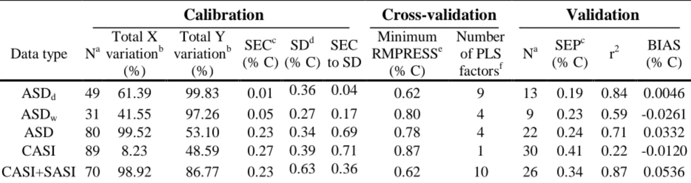
In order to relate the spectra with SOC content, stepwise and PLS regression were applied to each pre-treatment. Each model was sorted according to the SEC-to-SD ratio. Stepwise regressions yielded generally good SEC but SEP were not good enough to produce reasonable predictions (results not shown). SEP were high probably due to collinearity and over-fitting. These problems are usually fixed by the standard PLS procedure. Table 1 shows, for each data set, the PLS output statistics of the best model. Table 2 presents (combinations of) pre-treatment yielding the best model for each data set.
Results suggest that the calibration performed better when ASD is split into two classes of surface soil moisture. Validation shows closer results between the data sets. SEP varies between 0.19 (ASDd) and 0.24 (ASD) % of SOC
(Table 1). SEP is an important statistic since it assesses the ability of the model to predict the accuracy of SOC predictions at unsampled sites. Another useful statistic is the r2. When the r2 > 0.8, the model allows quantitative prediction while with an r² between 0.5 and 0.7, the model allows only rough estimates [15]. The r2 of ASDd was
greater than 0.8 denoting a reliable model. The r2 of ASDw and ASD were 0.59 and 0.71 respectively. Low
SEC-to-SD ratios indicate very good models for ASEC-to-SDd and ASDw. The SEC-to-SD ratio of ASD was not good enough to
make quantitative prediction. Attention should be paid to the results of ASDd and ASDw because there are large
differences between SEC and SEP whereas the values of SEC and SEP should be normally within 20 % of each other [15]. Bias, which is a measure of the difference between reference and predicted means, are low (ranging from –0.0261 to 0.0332 %). This implies that models using the data from the portable spectrometer do not systematically under- or overestimate carbon contents determined by the classic Walkley and Black method. The PLS regression on CASI data did not yield satisfying results (Table 1). The SEC-to-SD ratio is higher than 0.5 and the r2 is as low as 0.22. Furthermore, the SEP is greater than the SD, which implies that one obtains better results by simply using the mean of the calibration set as a predictor of the samples of the validation set than using the PLS model. The CASI+SASI data performed better than the CASI alone. This is most probably due to the wider spectral range of the CASI+SASI (444 to 2500 nm) compared to the CASI (405-950 nm) sensor and, possibly, due to the smaller pixel size (giving a more homogeneous surface) and the larger soil diversity in the other study area. The r2 is greater than 0.8, the bias is low and the SEC-to-SD ratio is below 0.5, indicating a good model. However, the SEP (0.34 %) is sensibly higher than the SEC.
The SEL of the carbon analysis using the Walkley-Black method has been approximately estimated at 0.15 % SOC. This number has to be used with caution because the calculation was based on five replicates. Nevertheless,
SEP of ASDd ASDw and CASI+SASI models are close to the SEL, suggesting that those portable NIR and
hyperspectral remote sensors could efficiently predict SOC. It should, nevertheless, be noted that the variance of SOC samples is small (SOC content varies between 1.99 to 4.27 %C), so that SEC and SEP are low as well. The SEP of all models appears to be too high in comparison with their SD, and therefore carbon contents of single samples estimated by the spectral techniques are probably less reliable. The spectral techniques should therefore at present not be used for precision farming studies or to accurately predict carbon contents for cartographic purposes. However, the low bias enables one to use NIR data, both ASD and CASI+SAI, to estimate population means with confidence using a large number of samples. In the next section it will be explained how the mean SOC content of a large number of samples can be used to estimate CO2 fluxes between the soil and the atmosphere.
Calibration robustness is an important issue when applying the spectral techniques to different areas or under different soil moisture status. The results from the different dates and pilot areas have yielded different calibration curves (Table 1). Therefore, at present calibration has to be developed simultaneously with the flight or during the field campaign in order to monitor the disturbing factors. This can be tedious. Moreover, soils in our study area are quite homogeneous (small variance in SOC content and similar soil texture) so that the models developed here are applicable only to our study area.
Table 1. Calibration and validation statistics for ASD, CASI, CASI+SASI data.
Calibration Cross-validation Validation
Data type Na Total X variationb (%) Total Y variationb (%) SECc (% C) SDd (% C) SEC to SD Minimum RMPRESSe (% C) Number of PLS factorsf Na SEP c (% C) r 2 BIAS (% C) ASDd 49 61.39 99.83 0.01 0.36 0.04 0.62 9 13 0.19 0.84 0.0046 ASDw 31 41.55 97.26 0.05 0.27 0.17 0.80 4 9 0.23 0.59 -0.0261 ASD 80 99.52 53.10 0.23 0.34 0.69 0.78 4 22 0.24 0.71 0.0332 CASI 89 8.23 48.59 0.27 0.39 0.71 0.87 1 30 0.41 0.22 -0.0120 CASI+SASI 70 98.92 86.77 0.23 0.63 0.36 0.62 10 26 0.34 0.87 0.0536 a
Number of samples in the calibration/validation procedure, b total predictor (X) or response (Y) variation (%) explained by the model, Standard Error of Calibration (SEC) and Prediction (SEP), d Standard Deviation, e Root Mean Predicted Residual Sum of Squares f smallest number of PLS factors determined by the cross-validation procedure.
Table 2. Best pre-treatments
Data type Mathematical pre-treatment type
ASDd
moving average with a window size of 3 bands, 1st derivative with a gap of 4 bands, keep one band every 10 nm ASDw
1st derivative with a gap of 2 bands, keep one band every 10 nm
ASD
Savitsky-Golay smoothing with a 3rd polynomial covering 40 nm, keep one band every 5 nm
CASI 1st devivative with a gap of 1 band CASI+SASI no pre-treatment
Table 3. SOC statistics per field
ID N Variance (t C ha –1) C.V. (t C ha-1) MDD (t C ha-1) n a A 7 11.83 0.03 5.55 8 B 10 166.36 0.14 17.00 105 C 11 21.24 0.06 5.76 14 L 11 149.37 0.12 15.28 95 M 11 52.20 0.08 9.03 34 N 11 124.04 0.12 13.93 79 O 11 21.05 0.07 5.74 14 P 11 101.08 0.14 12.57 64 Q 11 105.64 0.11 12.85 67 R 11 113.09 0.12 13.30 72 S 11 25.04 0.06 6.26 17 T 11 91.26 0.12 11.95 58 U 11 68.54 0.09 10.35 44 ALL 121 148.58 0.14 4.41 94 a
Number of samples in each group required to detect a stock change of 5 tC ha-1 resulting from a hypothetical management change.
4 APPLICATION
The major problem that soil C sequestration or emission studies have to cope with is the large spatial variability. The intra-field variability of the study area is in the same order of magnitude as the variability across all fields (Table 3). As a consequence, it requires many samples to calculate a SOC stock for an individual field. The MDD expresses the smallest amount of change that can be observed with a given spatial variability and sample number. Figure 2 shows MDD as a function of sample size and variance observed in the study area. The sampling intensity of our study (± 11 samples per field) yields MDDs ranging from 5.55 t C ha-1 to 17 t C ha-1. MDD of the entire study area (considered as a homogeneous spatial unit) is lower (4.41 t C ha-1) because of the larger sample size and comparable variance. In order to detect a SOC change as a result of management of 1 t C ha-1 yr-1 [21, 22] over a reasonable time period (5 years) applied across all fields, one requires 8-105 samples per field (table 3). To detect a similar change in the mean SOC stock in the entire study area, the number of samples required is in the same order of magnitude (n = 94).
Conventional sampling strategies are often too time consuming and expensive to provide such amount of samples. Such sampling intensity can only be achieved when studies are carried out on larger spatial units. Using airborne hyperspectral and portable NIR sensors, it becomes much more feasible to obtain these large number of samples. Since the bias is close to zero, NIR measurements can be used as a reliable estimator of the ‘true’ mean SOC content. Hyperspectral remote sensing is able to provide a large amount of samples (± 250 pixels per ha with a spatial resolution of 6m*6m) but is less accurate than hand held spectrometers. However, to use portable spectrometers is more time-consuming. Three important points should be kept in mind. Firstly, models have been calibrated in such a way that bias was minimized. The study area is small and soils or management type are quite homogeneous. This reasoning is thus only valid for similar soils and management type. It stresses the need of a larger study area, to calibrate models on a larger range of soils. Secondly, the MDD and its associated number of samples are calculated from parametric statistical theory which is based on the independence of the samples. It is well-known that the spatial correlation is quantified by the range of the semivariogram. For SOC, reported ranges in the semivariograms vary between 50 and 343 meters [23]. Nevertheless, as shown in Ref. [23], measurement should be made at least at the sub-meter or meter level to describe the variability of soil properties. Thirdly, these methods are only useful for arable soils. On the one hand, the airborne spectral techniques use the reflectance of the bare soils and on the other hand these techniques are not able to detect vertical gradients in SOC within the topsoil. For arable soils this is not a major problem since the topsoil is mixed during ploughing.
0 10 20 30 40 50 1 10 100 1000 10000 Sample size (n) M D D ( tC /h a ) var max var min var study area Management change
5 CONCLUSION
This study evaluates the application of NIRS in assessing the changes in SOC leading to C sequestration or emission. The handheld ASD spectrophotometer (350-2500 nm) produced more accurate estimations of SOC than hyperspectral remote techniques. ASD performed better when the data set was split in two classes representing soil surface moisture condition. Results from the airborne CASI sensor (405-950 nm) were not good enough to make quantitative prediction. The airborne CASI+SASI sensor (444 – 2500 nm) yielded reasonable results, probably due to its larger spectral range. It appears that there is no universal calibration due to various disturbing factors and different soil type. Calibration should be done simultaneous with the flight or the ground measurements to compensate for these disturbing factors. Calibration should also be done on a larger study area to increase soil diversity. Models showed low bias, suggesting that NIRS can efficiently estimate population mean. The large amount of samples provided by these techniques can sensibly reduce MDD, which is important for assessing small differences in SOC stocks between different dates. These differences can then be used to assess soil C sequestration or emission.
ACKNOWLEDGMENTS
This work was funded under the PRODEX programme of the European Space Agency (contract number C90166) and the support is gratefully acknowledged. We are grateful to the Vlaamse Instelling voor Technologisch Onderzoek (VITO) for organizing the flight campaign and carrying out the spectral measurements on the ground. We also wish to thank T. Stevens, C. Schmit and M. Bravin for their assistance during the field measurements.
REFERENCES
[1] TOURÉ,S. AND TYCHON,B., 2003: Estimation of soil organic matter by means of hyperspectral data analysis. Paper presented at the CASI-SWIR2002 Workshop, Bruges, September 4, 2003.
[2] MCCARTY,G.W. AND REEVES III,J.B., 2001: Development of rapid instrumental methods for measuring soil organic carbon. In: Lal, R. (ed.): Assement methods for soil carbon, pp. 371-380. Lewis, Boca Raton.
[3] MARTIN,P.D.,MALLEY,D.F.,MANNING,G. AND FULLER,L., 2002: Determination of soil organic carbon and nitrogen at the field level using near-infrared spectroscopy. Canadian Journal of Soil Science 82 (4), pp. 413-422. [4] REEVES III,J.,MCCARTY,G.W. AND MIMMO,T.,2002: The potential of diffuse reflectance spectroscopy for
the determination of carbon inventories in soils. Environmental Pollution 116 (S1), pp. 277-284.
[5] MCCARTY,G.W.,REEVES III,J.B.,REEVES,V.B.,FOLLETT,R.F. AND KIMBLE,J.M.,2002: Mid-infrared and near-infrared diffuse reflectance spectroscopy for soil carbon measurement. Soil Science Society America Journal 66 pp. 640-646.
[6] FIDÊNCIO,P.H.,POPPI,R.J., DE ANDRADE,J.C. AND CANTARELLA,H.,2002: Determination of organic matter in soil using near-infrared spectroscopy and partial least squares regression. Communications in Soil Science and Plant Analysis 33 (9-10), pp. 1607-1615.
[7] CHANG,C.-W. AND LAIRD,D.A.,2002: Near-infrared reflectance spectroscopic analysis of soil C and N. Soil Science 167 (2), pp. 110-116.
[8] SUDDUTH,K.A. AND HUMMEL,J.W.,1993: Soil organic matter, CEC, and moisture sensing with a portable NIR spectrophotometer. Transactions of the ASAE 36 (6), pp. 1571-1582.
[9] BEN-DOR,E.,PATKIN,K.,BANIN,A. AND KARNIELI,A., 2002: Mapping of several soil properties using
DAIS-7915 hyperspectral scanner data - a case study over clayey soils in Israel. International Journal of Remote Sensing 23 (6), pp. 1043-1062.
[10] PALACIOS-ORUETA, A. AND USTIN, S. L., 1999: Remote sensing of soil properties in the Santa Monica Mountains. I. Spectral analysis. Remote Sensing and Environment 65 pp. 170-183.
[11] PETIT,C.C. AND LAMBIN,E.F.,2002: Long-term land-cover changes in the Belgian Ardennes (1775-1929): Model-based reconstruction versus historical maps. Global Change Biology 8 (7), pp. 616-631.
[12] WALKLEY,A. AND BLACK,I.A.,1934: An estimation of the Degtjareff method for determining soil organic
matter and a proposed modification of the chromic acid titration method. Soil Science 37 pp. 29-37.
[13] SAVITZKY,A. AND GOLAY,M.J.E., 1964: Smoothing and differentiation of data by simplified least squares procedures. Analytical Chemistry 36 (8), pp. 1627-1638.
[14] STEINER,J.,TERMONIA,Y. AND DELTOUR,J., 1972: Comments on smoothing and differentiation of data by simplified least square procedure. Analytical Chemistry 44 (11), pp. 1906-1909.
[15] COÛTEAUX,M.-M.,BERG,B. AND ROVIRA,P., 2003: Near infrared reflectance spectroscopy for determination of organic matter fractions including microbial biomass in coniferous forest soils. Soil Biology and Biochemistry 35 (12), pp. 1587-1600.
[16] GARTEN, C. T. AND WULLSCHLEGER, S. D., 1999: Soil carbon inventories under a bioenergy crop
(Switchgrass): measurement limitations. Journal of Environmental Quality 28 pp. 1359-1365.
[17] CONANT, R.T., SMITH,G. R. AND PAUSTIAN,K., 2003: Spatial variability of soil carbon in forested and cultivated sites: implications for change detection. Journal of Environmental Quality 32 pp. 278-286.
[18] HOMANN,P.S.,BORMANN,B.T. AND BOYLE,J.R., 2001: Detecting treatment difference in soil carbon and nitrogen resulting from forest manipulations. Soil Science Society America Journal 65 (2), pp. 463-469.
[19] YANAI,R.D.,STEHMAN,S.V.,ARTHUR,M.A., PRESCOTT,C. E.,FRIEDLAND,A.J., SICCAMA,T.G. AND
BINKLEY,D., 2003: Detecting change in forest floor carbon. Soil Science Society America Journal 67 (5), pp.
1583-1593.
[20] CAMPBELL,M.J., JULIOUS,S.A. AND ALTMAN,D.G., 1995: Estimating sample sizes for binary, ordered categorical, and continuous outcomes in two group comparisons. British Medical Journal 311 pp. 1145-1148. [21] GUO,L.B. AND GIFFORD,R. M., 2002: Soil carbon stocks and land use change: a meta analysis. Global Change Biology 8 pp. 345-360.
[22] POST,W.M. AND KWON,K.C.,2000: Soil carbon sequestration and land-use change: processes and potential. Global Change Biology 6 pp. 317-327.
[23] SOLIE, J. B., RAUN, W. R. AND STONE, M. L., 1999: Submeter spatial variability of selected soil and Bermudagrass production variables. Soil Science Society America Journal 63 pp. 1724-1733.