Quelques utilisations de la densité GEP en analyse
bayésienne sur les familles de position-échelle
par
Alain Desgagné
Département de mathématiques et de statistique Faculté des arts et des sciences
Thèse présentée à la Faculté des études supérieures en vue de Fobtention du grade de
Phi1osophia Doctor (PhD.) en statisticiue
mai 2005
K P
îr,1
J)
fln5
de Montréal
Direction des bibliothèques
AVIS
L’auteur a autorisé l’Université de Montréal à reproduire et diffuser, en totalité ou en partie, par quelque moyen que ce soit et sut quelque support que ce soit, et exclusivement è des fins non lucratives d’enseignement et de recherche, des copies de ce mémoire ou de cette thèse.
L’auteur et les coauteurs le cas échéant conservent la propriété du droit d’auteur et des droits moraux qui protègent ce document. Ni la thèse ou le mémoire, ni des extraits substantiels de ce document, ne doivent être imprimés ou autrement reproduits sans l’autorisation de l’auteur.
Afin de se conformer à la Loi canadienne sur la protection des renseignements personnels, quelques formulaires secondaires, coordonnées ou signatures intégrées au texte ont pu être enlevés de ce document. Bien que cela ait pu affecter la pagination, il n’y a aucun contenu manquant. NOTICE
The author 0f this thesis or dissertation has granted a nonexclusive license allowing Université de Montréal to reproduce and publish the document, in part or in whole, and in any format, solely for noncommercial educational and research purposes.
The author and co-authors if applicable retain copyright ownership and moral rights in this document. Neither the whole thesis or dissertation, nor substantial extracts from it, may be printed or otherwise reproduced without the author’s permission.
In compliance with the Canadian Privacy Act some supporting forms, contact information or signatures may have been removed from the document. While this may affect the document page count, it does flot represent any loss of content from the document.
Facilité des études stipérielires
Cette thèse intitulée
Quelques utilisations de la densité GEP en analyse
bayésienne sur les familles de position-échelle
présentée par
Alain Desgagné
a été évaluée par un jury composé des personnes suivantes Roch Roy (président-rapporteur) Jean-François Angers (directeur de recherche) Louis Doray (membre du jury) Liqun Wang (examinateur externe)
Fran çois BeÏÏavance (représentant du doyen de la FES)
Thèse acceptée le: 30 mai 2005
RÉSUMÉ
L’utilisation des distributions à ailes relevées est tin outil précieux clans le développement de méthodes bayésiennes robustes, limitant l’influence des valeurs aberrantes sur l’inférence a posteriori. Dans un premier temps, le comportement de la densité a posteriori du paramètre de position est étudié, lorsque l’échantillon contient des valeurs aberrantes. La notion de p-crédence à gauche et à droite est introduite afin de caractériser et ordonner les ailes gauche et droite d’une grande classe de densités, en comparant leurs ailes à celles d’une densité de puissance d’exponentielles généralisée (CEP).
Dans le premier article, la densité GEP est proposée comme fonction d’impor tance clans les simulations IVionte Carlo clans le contexte d’estimation des moments a posteriori du paramètre de position. Cela permet d’obtenir des résultats fiables et efficaces, même s’il y a des sotirces d’information conflictuelles. La simulation d’observations provenant d’une densité GEP est aussi discutée.
Dans le cletixiènie article, des conditions sur les ailes de la densité apriori et de la vraisemblance, basées sur la p-crédence à gauche et à droite, sont établies afin de déterminer la proportion d’observations pouvant être rejetées lorsque celles-ci sont extrêmes. Il est démontré que la distribution aposteriori converge en loi vers la distribution a posteriori obtenue à partir de l’échantillon excluant, les valeurs aberrantes, lorsque ces dernières tendent vers pltis ou moins l’infini, à n’importe quel taux. Un exemple de combinaison de prévisions du rendement de l’indice
SP 500 est présenté.
Finalement, clans le troisième article, le comportement de la densité a poste
riori du paramètre d’échelle est étudié lorsque l’échantillon contient des valeurs aberrantes et que les observations sont positives. La notion de log-crédence à
gauche et à droite est introduite afin de caractériser les ailes gauches et droites d’une densité définie sur R+. Des conditions sur les ailes de la densité a priori et de la vraisemblance, basées sur la log-crédence à gauche et à droite, sont établies afin de déterminer la proportion d’observations pouvant être rejetées lorsque celles-ci sont extrêmes (observations très petites ou grandes par rapport aux autres). Un exemple de combinaison de prévisions de la volatilité des rendements de l’indice S&P 500 est présenté.
MOTS CLÉS:
Inférence bayésienne, Modèle à ailes relevées, famille de puissance d’exponen tielles généralisée, Crédence, Valeurs aberrantes, Paramètre de position, Para mètre d’échelle, Convergence en loi, Simulations iVionte Carlo, Fonction d’impor tance
S UM1VIARY
The use of heavy-tailed distributions is a valuahie tool in cÏeve1opiig robust Bayesian proceclures, limitïng the influence of outiiers on posterior infereilce. The behavior of the posterior clensit.y, when the sample contains outiiers, is ftrst in vestigateci for the location parameter. The notion of left anci right p-credence is introcluceci to characterize anci to orcler the Ïeft anci right tails of a large class of clensities hy comparing their taiÏs t.o those of the generalizeci exponential power
(GEP) density.
In the flrst paper, the GEP density is proposed as an importance function in IVionte Carlo simulations in the context of estimation of posterior moments of a location parameter. It alÏows us to obtain reliable ancÏ effective resuits, even if there are conflicting sources of information. Simulation of observations from the CEP clensity is also acldressed.
In the second paper, conditions on the tails of the prior anci the likelihood, using left anci right p-creclence, are establisheci to cletermine the proportion of observations that can 5e rejected when they are consiclereci extrerne. It is shown that the posterior distribution converges in law to the posterior that woulcl 5e obtaineci from the rechiced sample, exclucling the outiiers, as they tend to plus or minus inflnity, at any given rate. An example of combination of preclictions of the S&P 500 iilclex return is presenteci.
Finally, in the thirci paper, the behavior of the posterior clensity of the scale parameter is investigatecl when the sample contains outiiers anci only positive ob servations. The notion of left anci right log-creclence is introcluceci to characterize respectively the left anci right tails of a clensity cleflnecl on R+. Conditions on the
tails of the prior anci the likelihooci, using left anci right log-crecLence, are establi shed to determine the proportion of ohservatioiis that can be rejecteci whell they are considered extrerne (observations very srnall or large relatively to the other ones). An example of combination of preclictions of the voÏatility of the SP 500 index return is presentecÏ.
KEY WORDS:
Bayesian inference. Heavy-tailecl mocleling, Generalizeci exponential power family, Outiier, Credence, Location parameter, Scale parameter, Convergence in law, Monte Carlo simulations, Importance sampling
REMERCIEMENTS
Je tiens d’abord à remercier chaleureusement mon directeur de recherche Jean François Angers. Par ses qualités humaines, il a contribué grandement à créer un climat de travail clans lequel il fut très agréable cl’évolller. lI m’a proposé un projet de recherche que
j
‘ai adoré et il m’a accompagné tout au long de ceprojet en partageant généreusement son expertise et son expérience. Aussi, j’ai apprécié grandement son leadership, cfui m’a permis de bénéficier à la fois de toute l’autonomie nécessaire pour me développer comme chercheur, de sa grande disponibilité et de son appui clans les moments plus difficiles.
Je remercie également les membres du jury pour la lecture de ma thèse ainsi
que pour les améliorations qu’ils ont apportées.
Je remercie les professeurs, les étudiants et le personnel du département que
j’ai côtoyés durant ces années, pour toutes les conversations échangées et les bons
moments passés ensemble qui ont permis de rendre mon doctorat très agréable. Plus particulièrement, je veux remercier les professeurs Robert Cléroux pour
le support qu’il m’a donné au début de mon doctorat et Louis Doray pour les
conversations sur le monde de l’actuariat et son appui dans ma recherche fruc
tueuse d’un poste de professeur.
Je tiens aussi à remercier plus particulièrement quelques collègues étudiants pour leur amitié et les très bons moments partagés ensemble t Alexancire Leblanc, Pierre Lafaye de Micheaux, Alice Dragomir, Pascal Croteau et Jean-François Bon dreau.
Je veux souligner l’apport financier important que
j
‘ai obtenu de la Part du CRSNG (Conseil de recherches en sciences naturelles et en génie du Canada),du FQRNT (Le Fonds cinébécois de la recherche sur la nature et les technolo gies), de la SOA (Societv of Actuaries), du Département de mathématiques et de statistiqile de l’Université de Montréal ainsi que de mon directeur de recherche.
Finalement, un grand merci à ces personnes qui ont m’ont aidé indirectement dans ce projet mes parents Yves et Pauline, mes deux soeurs Chantai et Manon et la grande famille que
j
‘aime beaucoup, Ingrid de Lafont aine, Anne-IViarie Castilloux, Marie Flagollet, Louis Beaudoin, Jean-Guy St-Jean et Jean-Christophe
TABLE DES MATIÈRES
Résumé . iv
Summary . vi
Remerciements viii
Sigles et abréviations xiv
Liste des figures xv
Liste des tableaux xvi
Introduction f Contexte bayésien 2 Robustesse 3 Densité CEP 5 Premier article 6 Deuxième article 6 Troisième article 8 Bibliographie 9
Chapitre 1. Importance Sampling with the Gerieralized Exponential
Power Density 12
1 2 Generalizeci exponential p ower cÏensity ancÏ dominance relation using
p-crecÏence 13
1.2.1. Generalizeci exponential power cïensity 14
1.2.2. Dominance relation using p-creclence 15
1.3. Importance sampling 1$
1.3.1. Setting 1$
1.3.2. The uniform part of the importance function 19
1.3.3. Characterization of the posterior using p-creclence 19
1.3.4. Simulation of observations from the GEP density 20
1.3.5. Selection of parameters of the importance function 23
1.4. Example 23
1.4.1. Setting 23
1.4.2. Data 24
1.4.3. The importance ftmctions 24
1.4.4. Resuits 25
1.5. Conclusion 29
1.6. Acknowledlgmellts 29
1.7. References 29
Chapitre 2. Outiiers and choice of the prior for location parameter
inference 31
2.1. Introduction 32
2.2. Outliers rejection using p-credlence 33
2.2.1. A measure of the tails : left anci right p-creclences 33
2.2.2. Outiiers rejection using left anci right p-creclences 35
2.2.3. Conflicting information with one observation 3$
Conditions of thickness ancÏ reguÏarity for the tails of a clensity Outlier rejection 2.7. Ackuowiecigments 44 44 45 46 47 47 48 52 55 56 57 59 62 63 69 2.8. References 69
Chapitre 3. Otitiiers for scale parameter inference and positive
observations 71
3.1. Introduction 72
3.2. Outiiers rejection using log-credence
3.2.1. A measure of the tails left and right log-creclences 3.2.2. Outiiers rejection using left anci right log-creclences
40 42 2.3.1. 2.3.2. 2.4. Example 2.4.1. First case 2.4.2. Second case 2.4.3. Third case 2.5. Conclusion 2.6. Appenclix t Proofs
2.6.1. Proof of resuit a) of Theorem 2 2.6.2. Proof of Lemma 3
2.6.3. Proof of resuit h) of Theorem 2 2.6.4. Proof of resuit c) of Theorem 2 2.6.5. Proof of resiit cl) of Theorem 2 2.6.6. Proof of resuit e) of Theorem 2 2.6.7. Proof of Lemma 11
2.6.8. Proof of Theorem 1
73 73 76
3.3.1. Coilditions of thickness and regularity for the tails of a density
dened on R 81
3.3.2. Outiler rejection 22
3.4. Example 84
3.4.1. Context $4
3.4.2. Exponential transformation of symmetric densifies defineci on R 85
3.4.3. Data 86
3.4.4. Resuits 87
3.5. Conclusion $8
3.6. Appendix : Proofs $9
3.6.1. Proof of resuÏt a) of Theorem 4 89
3.6.2. Proof cf Lenima 15 93
3.6.3. Proof of resuif b) of Theorem 4 97
3.6.4. Proof of resuif e) cf Theorem 4 9$
3.6.5. Proof of resuif cl) of Theorem 4 99
3.6.6. Proof of resuit e) of Theorem 4 101
3.6.7. Proof of Lemma 23 104
3.6.8. Proof of Theorem 3 106
3.7. Acknowledgments 112
3.8. References 112
SIGLES ET ABR1VIATIONS
cclf t Fonction cmrnilative de distribution
GEP : Puissance cl ‘exponentielles généralisée
S&P 500 : Indice boursier Standard Poors 500
• j
t Valeur absolue t Nombres réelst Nombres réels positifs
N t Nombres naturels t Convergence en loi
t Espérance
Var[.j t Variance
I[[a] t function indicatrice de l’ensemble {a}
p-cred(f) t P-crédence de la densité
f
p_cred+(f) t P-crédence de l’aile de droite de la densité
f
p-cred
(f)
t P-crédence de l’aile de gauche de la densitéf
log_cred±(f) t Log-créclence de l’aile de droite de la densité
f
LISTE DES FIGURES
1.1 The posterior and the importance functions ta) for the first example,
(b) for the second example; tire clensities -— O) for i = O 5 (e)
for tire first example, (cl) for tire second example 27 1.2 The weights (divicleci by their maximum) over their corresponcling
observation for each importance function (a) for tire ftrst example (b)
LISTE DES TABLEAUX
1.1 five types of the GEP density 15
1.2 Normalizing constant anci moments of the GEP clensity 16
1.3 Simulation of an observation z from a GEP density On (zo,oo), (note
w U[0,
11)
211.4 Proposais when direct simulation from p(zVy, , c,/3,zo) is not possible 22 1.5 Stanclarc[ error anci 95% confidence interval for tue estimat,e E(Ox)
after 10,000 simulations, for the first example 25
1.6 Standard error anci 95% confidence interval for the estimate x)
after 10,000 simulations, for the second example 26
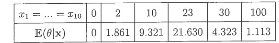
2.1 Tire posterior mean E(&x) for different values of .x10, when (x =
(—2,—2, —1, —1,0,1, 1,2,2) 45
2.2 Tire posterior mean E(9x) for different vailles of x6 = 17 = 19 =
ho, when (Ii, I) = (—1, —1, 0, 1, 1) 46
2.3 The posterior mean E(6x) for different values of 16 7 = =
x11, when (hi, ..., x) (—1, —1, 0, 1, 1) 46
2.4 Tire posterior mean E(&x) for different values of i = xo, when 47
3.1 Prior and experts’ preclictioirs ancl 95% confidence intervals $6
Avec la progression de l’informatisation clans ]es entreprises et les institu
tions gouvernementales, de plus en plus de hases de données sont maintenant
disponibles. Une mine d’information souvent se cache clans ces données et le dé veloppement cl’ outils statistiques permettant de les analyser devient nécessaire.
Par exemple, l’efficacité cl’tm médicament peut être démontrée en utilisant l’in
formation contenue clans les bases de données de la Régie de, l’assurance-maladie du Québec, ou le risclue d’accident automobile d’un assuré peut être mieux éva
lué en utilisant l’information contenue clans la base de données cl’tme compagnie
d’assurance, ce qui permet de mieux évaluer la portion de la prime d’assurance
due au risque.
IJne autre conséquence de l’avènement d’ordinateurs de plus e plus puissants
est la possibilité accrue de développer des outils statistiques de plus en plus per
formants. Plusieurs approches statistiques, utilisant par exemple les simulations
ou le calcul numérique, sont maintenant utilisables via l’ordinateur afin d’analyser ces bases de données.
Une de ces approches statistiques est l’inférence bayésienne. Elle consiste es
sentiellement à combiner l’information provenant des données avec de l’informa tion o. pr%oTz réputée indépendante des données, pour en tirer de l’information o.
posteriori. L’approche bayésienne nécessite souvent des calculs numériques inten
sifs et le développement des ordinateurs a sans doute contribué à son essor. Un des critères de performance recherché en statistique est la robustesse des
modèles face aux valeurs aberrantes. Pour la plupart des échantillons, un mo
petit ne pins être adéquat dès qu’une ou plusieurs valeurs extrêmes ou aberrantes
apparaissent clans les données.
Le but de cette thèse est de développer des outils statistiques bayésiens ro bustes, qui demeurent efficaces même si des valeurs aberrantes viennent contami ner les données. Le contexte bayésien est décrit plus en détail dans la prochaine section.
CONTEXTE BAYÉSIEN
Soient n variables aléatoires X1, ...,X conditionnellement indépendantes
é-tant donné le paramètre 8. La densité conditionnelle de X0 est donnée par avec 8
e
et X , i = 1,..., n, oùe
et sont des sous-ensembles de R. Notez que l’espace paramétriquee
peut être multidimensionnel, mais seul le cas unidimensionnel est considéré dans cette thèse. L’inférence est faite sur le paramètre & à partir des données observées x, ..., x,,. Notez que dans l’approche classique (fréquentiste), une nouvelle expérimentation produirait un nou vel échantillon x1, ...,x et la valeur (inconnue) de 8 resterait la même, tandis que
clans l’approche bayésienne, une nouvelle expérimentation produirait une nou velle valeur de 8. L’aspect aléatoire dans l’approche bayésienne est donc mis sur le paramètre 8 plutôt que sur les données.
L’information a priori sur & est donc intégrée dans le modèle par l’entremise d’une loi a priori sur 9, dénotée par n(&) (voir DeGroot, 1970). Il est donc possible d’inférer sur le paramètre O sans même observer de données, à l’aide de la loi a prio’ri. Le paradigme bayésien consiste à mettre à jour cette densité e priori en y intégrant les observations x1, ..., x,, par le théorème de Bayes. Rappelons que
par le théorème de Bayes, Pr[AB] = Pr[BA] Pr[A]/ Pr[B], où A et B sont deux sous-ensembles d’un espace échantillonal S, c’est-à-dire A C S et B C S. Nous obtenons alors la densité e posteriori de 8, dénotée par n(9xi, ..., x,) et donnée
par
r(O)
fl f(x&)
...,x)
OÙ ?Tl(xi, ...,X,,) fe n(9)
flL
f(xO)dO est la densité marginale conjointe decompte à la fois de l’information a priori et des données. Notez que la densité a posteriori est proportionnelle au produit des densités de toutes les sources d’in formation. Selon le critère d’optimisation (fonction de coûts) choisi, le paramètre O peut être estimé par l’espérance, la médiane 011 le mode a poster’o’ri de 9.
Dans cette thèse, nous nous intéressons aux densités des observations qui font partie cl’ulle famille de position-échelle. Soit une variable aléatoire Y ayant comme densité f(y), alors la densité de X = o-Y +ti, étant donné ,u et u connus, est donnée par u1f([x —
i]/u), où tt est le paramètre de position et u > O est le paramètre d’échelle. Nous disons que la densité de X est une famille de position-échelle, ou simplement une famille de position si o est fixé ou encore une famille d’échelle si i est fixé. Une variation du paramètre de position entraîne une translation de la densité et une variation clti paramètre d’échelle entraîne un étirement ou un rétricissement de la densité. Nous aborderons clans cette thèse la famille de position dans les deux premiers articles et la famille d’échelle clans le troisième article. Le paramètre 9, donné dans le cac[re bayésien, sera donc un paramètre de position ou un paramètre d’échelle.
ROBUSTESSE
Ui exemple souvent présenté comme introduction à la statistique bayésienne consiste à faire l’hypothèse que la densité a priori et la fonction de vraisemblance (densité des observations) sont représentées par des densités normales. Si est une observation provenant d’une population normale avec une moyenne donnée par O et une variance de 1, ce qui est dénoté par N(0, 1), et que la densité a priori de O est N(O, 1), alors on peut démontrer que la densité a posteriori de O est N(x/2, 1/2). Notez que la densité de l’observation appartient à une famille de position. Selon l’information e priori, la distribution du paramètre O est centrée en O, tandis que l’observation est donnée par x. La densité e posteriori est centrée en /2, ce clui représente un compromis entre les deux sources d’information. La densité eposteriorz de O est proportionnelle au produit de la densité epriori et de la vraisemblance considérée comme une fonction de O, soit le produit d’une densité N(O, 1) et d’une densité AT(r, 1). Rappelons que la densité normale est unimoclale
et symétrique par rapport à sa moyenne. Une petite variance indique une grande certitude de la source d’information et vice-versa. Par exemple. selon l’information
a prwrz, il y a moins d’une chance sur 1000 que 0 soit supérieur à 3,3, puisque la densité de O est N(0, 1). De la même façon, selon la vraisemblance, il y a moins
d’une chance sur 1000 que 0 — x soit supérieur à 3,3. Le compromis de
semble naturel si les cieux sources d’information sont compatibles. Par exemple si
= 3, la densité a posterior? fera un compromis avec une moyenne de x/2 = 1, 5,
ce qui est en accord à la fois avec l’information a priori et avec la vraisemblance. Toutefois, si 10 et que la densité a posteriori fait. un compromis avec une moyenne de x/2 5, ce n’est pas souhaitable, puisqu’il est eu désaccord à la fois avec l’information a priori (moins d’une chance sur 1000 d’être inférieur à -3,3 ou supérieur à 3,3) et avec l’observation (moins d’une chance sur 1000 d’être inférieur à 6.7 ou supérieur à 13.3). Il serait souhaitable clans ce cas d’écarter la source d’information jugée la moins fiable et que la ciensité a posteriori se rapproche de la source d’information avant la plus grande crédibilité en cas de conflit Si toutefois nous faisons l’hypothèse que la densité a priori est représentée par une densité ayant des ailes suffisamment relevées, telle la densité Stuclent-t, et que la vraisemblance est toujours représentée par une densité normale, le conflit sera réglé en faveur de la fonction de vraisemblance.
L’utilisation des densités à ailes relevées est un outil important clans le clé veloppement de méthodes bayésiennes robustes, limitant l’influence des valeurs aberrantes sur l’inférence a posteriori. Le rejet de valeurs aberrantes n d’abord été décrit par De Finetti (1961), clans le cas le plus simple où il n’y a qu’une observa tion avec une moyenne de 0. Des résultats théoriques ont été donnés par Dawici (1973) et Hill (1974). O’Hagan (1979) a considéré le rejet. de valeurs aberrantes clans un échantillon et O’Hagan (198$) a considéré une modélisation bayésienne plus générale basée sur les densités St.uclent—t. O’Hagan (1990) a introduit la no tion de crédence pour caractériser et ordonner des ailes de densités symétriques ayant un comportement de type polynomial, telle la densité Stuclent-t. Il a éga lement donné des résultats de rejet de valeurs aberrantes basés sur la crédence. Cette notion a été généralisée à la p-crédence par Angers (2000) afin d’englober
une plus grande classe de densités. D’autres auteurs ont également abordé le re jet de valeurs aberrantes, par exemple Meinholci et Singpurwalla (1989), Angers et Berger (1991), Carlin et Poison (1991), Angers (1992), Fan et Berger (1992),
Geweke (1994) et Angers (1996).
DENsITÉ
GEP
La p-crédence caractérise les ailes de densités symétriques en comparant ses ailes à celles d’une densité de référence appelée famille de puissance cl’exponen tielles généralisée (CEP). La forme générale de la densité CEP, telle qu’introduite par Angers (2000), est donnée par
p(z,
5, c, ,zo)
= K(7, 5,c,
,zo)
exp {—5max(z ,x
max(z,zo)
log [max(z,zo)]
[e_1
z°
logIz; si zI
>z0,
z
logz0;
siIz <z0,
où
z e
R, > 0, 5> 0 (nous posons S = O lorsque 0),e
R,e
R,z0
> Oet K(7, 5,,3,
z0)
est la constante de normalisation.La densité CEP comprend un terme exponentiel, poïyi;omial et logarithmique. Elle est symétrique par rapport à O et constante entre
—zo
etz0.
Les quatre autres paramètres ‘y, 5, o,/3 déterminent le comportement des ailes. La plupartdes densités connues définies sur R ou stir R ont le même comportement dans les ailes ciue la densité CEP, ce qui en fait
une
densité de référence utile. Aussi,comme la robustesse est liée principalement à l’épaisseur des ailes des densités, la densité CEP s’avère un outil puissant pour développer des méthodes statistiques bayésiemes robustes.
Dans cette thèse, trois utilisations de la densité GEP en robustesse bayésienne
PREMIER ARTICLE
Dans le premier article, intitulé Importance Sarnpling with the Generalized Exponentiat Power Density, la densité CEP est proposée comme fonction cl’im portance clans les simulations I\’Ionte Carlo, clans le contexte de l’estimation des moments a posteriorz du paramètre de position. Il est possible de caractériser les ailes de la densité e posteriori par la p-crédence (voir Angers, 2000), ce qui
permet de choisir les paramètres de la densité CEP de façon à ce que les ailes de la fonction d’importance soit légèrement pltis relevées ou équivalentes à celles de la densité e p08terOTZ. Aussi il est possible de simuler des observations à partir de la densité GEP, ce qui est abordé dans l’article. Souvent le choix d’tme fonction d’importance se fait sur la base du cas par cas. Il est toutefois possible, avec la densité GEP, de choisir une fonction d’importance selon une méthode qui est la rhème peu importe les choix de la densité e priori et de la vraisemblance, en autant que leur p-crédence soit définie. Aussi la présence de valeurs aberrantes ne compromet pas l’efficacité de cette méthode, •ce cmi n’est souvent, pas le cas pour des choix de fonctions d’importance cd [roc. D’autres approches permettant de choisir une fonction d’importance, basées sur la cliscrétisation aléatoire par exemple (voir Fu et Wang, 2002), peuvent aussi être efficaces. Il s’agit souvent de faire un compromis judicieux entre l’efficacité et la simplicité, et c’est clans cet esprit que la méthode proposée dans le premier article a été construite.
Dans les deuxième et troisième articles nous nous intéressons aux conditions portant sur la densité a priori et sur la vraisemblance qui sont suffisantes pour que la densité e posteriori rejette les valeurs aberrantes. Dans le deuxième article, la vraisemblance est une famille de position, tandis ciue dans le troisième, elle est une famille d’échelle. Les conditions portent essentiellement sur l’épaisseur des ailes.
DEuxIÈME ARTICLE
Dans le deuxième article, intitulé Outiiers crut choice of the prior for Ïocatiomm parameter inference, la p-crédence est d’abord généralisée afin de caractériser les ailes de gauche et de droite d’une densité définie sur les réels, ce qui permet de
considérer la robustesse en présence de densités asymétriques. Dans un tel cas, une observation trop petite par rapport aux autres pourrait par exemple être rejetée, mais ne le serait pas si elle était trop grande, ou vice-versa. Dans un premier temps, les conditions de robustesse sont exprimées à l’aide de la p-crédence. Ces conditions sont relativement faciles à vérifier, contrairement à celles énoncées clans Dawicl (1973) par exemple. Comme la p-crédence est définie pour la plupart des densités connues, ces conditions sont d’un grand intérêt en pratique. Rappelons que les résultats de O’Hagan (1990) ne s’appliquent que pour les densités ayant un comportement de type polynomial dans les ailes, tandis ciue les résultats clii deuxième article s’appliquent en pulls pour les densités ayant un comportement de type exponentiel et logarithmique clans les ailes.
Les résultats de robustesse sont donnés sous forme de convergence en loi. Si les conditions sont respectées, il est démontré que la densité e posteriori converge en loi vers la densité a posteriori que nous aurions obtenue à partir d’un échantillon excluant les valeurs aberrantes, à mesure que celles-ci tendent vers plus ou moins l’infini. D’une part ces résultats sont plus forts que ceux donnés clans O’Hagan (1990) et Angers (2000), cmi ont démontré que le ratio des densités a posteriori avec l’échantillon complet et avec celui excluant les valeurs aberrantes est borné par des constantes positives, pour n’importe quelle valeur finie du paramètre de position. Le prix pour obtenir la convergence en loi a été d’ajouter une condition stir la régularité des ailes de la densité e priori et de la vraisemblance. Toutefois, cette condition est satisfaite pour la plupart des lois connues. D’autre part, les résultats de convergence sont donnés lorsqu’on est en présence d’un échantillon comportant possiblement une ou plusieurs valeurs aberrantes clui tendent vers
plus ou moins l’infini, et ce à n’importe quel taux donné.
Dansun deuxième temps, les conditions sont présentées d’une façon plus géné rale, sans utiliser la p-crédence. Même si leur utilisation en pratique devient moins intéressante, elles demeurent relativement simples. L’interprétation des conditions devient toutefois plus aisée, puisclue l’influence de chaque aile de la densité epriori
et de la vraisemblance sur le rejet des valeurs aberrantes peut être observée. Es sentiellement, un groupe de valeurs aberrantes tendant vers l’infini sera rejeté
si l’aile de gauche de la densité proportionelle au produit de leurs densités est
suffisamment relevée et plus relevée que l’aile de droite de la densité proportion
nelle au produit des densités des observations non aberrantes et de la densité a
priori. Le rejet des valeurs aberrantes tendant vers moins l’infini est similaire, sauf
que le rôle des ailes de gauche et de droite est inversé. Le paramètre de position
est la variable aléatoire, les observations étant considérées fixes. Les résultats de
convergence sont valides quelque soit le taux auquel les valeurs aberrantes tendent
vers pitis ou moins l’infini. Quoiqu’ayant peu d’intérêt en pratique, il serait pos sible d’ajouter d’autres conditions de convergence si le taux auquel chaque valeur
aberrante tend vers plus ou moins l’infini était spécifié.
TROISIÈME ARTICLE
Dans le troisième article, intitulé Outiiers for scate parai eter inJrence and
positive observations, la robustesse est étudiée lorsque la densité des observations
est une famille d’échelle et que l’inférence est faite sur un Daramètre d’échelle.
Jusqu’à présent, aucun article n’a été publié sur ce sujet. Lorsque les observations sont considérées positives, il s’agit essentiellement de transposer les résultats du deuxième article par une transformation exponentielle (ou logarithmique si on fait
le chemin inverse). Le paramètre de position devient un paramètre d’échelle et le
domaine réel devient un domaine réel positif. Les conditions, résultats et preuves
de robustesse sur le paramètre d’échelle sont toutefois présentés indépendemment de leur contrepartie du monde du paramètre de position. En effet, nous aurions
pu être tentés de ne pas présenter le détail des preuves en référant simplement au deuxième article et en précisant qu’une transformation exponentielle doit être
effectuée. Quoique facile à faire pour certaines parties des preuves, il s’est avéré
d’une part qu’il n’est pas du tout trivial en général de transposer les preuves, et
cl’atitre part ciue des éléments nouveaux doivent souvent être apportés.
D’abord la notion de log-crédence est introduite, qui consiste à comparer les ailes cl’mne densité définie sur les réels positifs à celle d’une diensité log GEP. La
densité log G EP est définie simplement comme une transformation exponentielle
une densité GEP (un cas particulier correspond aux lois normale et log-normale). Tout comme clans le cas de la p-crédence, le comportement des ailes de densités de type polynomial et logarithmique est considéré clans la log-crédence, mais le comportement exponentiel est modifié et un terme logarithme de logarithme y est ajouté.
L’interprétation cte l’aile de gauche est un peu différente car le domaine est borné à gauche par O. L’aile de gauche peut monter vers l’infini, descendre vers O ou se diriger vers une constante positive. On dira par exemple que l’aile de gauche sera plus relevée si elle monte vers l’infini que si elle descend à O. La log-créclence peut mesurer l’aile de gauche d’une densité définie sur les réels positifs, ce que la p-crédence ne peut faire. L’interprétation des conditions et des résultats de convergence pour le cas du paramètre d’échelle est similaire au cas du paramètre de position. Les ailes des densités des valetirs aberrantes doivent être aussi suf • fisamment relevées, mais encore plus relevées que dans le cas du paramètre de • position.
Le cas du paramètre d’échelle quand les observations sont réelles n’est pas considéré clans cet article, mais il est facile de le faire en généralisant les résultats en iltilisant la symétrie par rapport à l’origine. Dans le cas d’observatioiis réelles, il n’y a toutefois pas de valeurs aberrantes près de O, et il en résulte cïue l’aile de gauche de la densité e priori du paramètre d’échelle n’a plus d’influence sur la robustesse. Une suite à ces travaux de thèse est en cours, où le cas de la famille de position-échelle est considéré, lorsque les données sont réelles.
BIBLIOGRAPHIE
ANGERS, J.-F. (1992) Use of Student-t prior for the estimation of normal
A computational approach, Bayesian Statistic IV ecis. Bernardo, J.1VI., Berger, J.O., Davici, A.P., and $mith, A.F.M., New York Oxford University Press, pp. 567-575.
ANGERS, J.-F. (1996) Protection against outliers using a symmetric stable law prior, IMS Lecture Notes - Monograph Series, Vol. 29, pp. 273-283.
ANGERS, J.-F. et BERGER. J.O. (1991) Rohust hierarchical Bayes estimation
of exchangeable means, The Ganadiau Journal of Statistics, 19, 39-56.
CARLIN, B. et POLSON, N. (1991) Inference for nonconjugate Bayesian moclels using the Gibhs sampler, Tire Canaclian Journal of Statist?cs, 19, 399-405. DAWID, A.P. (1973) Posterior expectations for large observations, Biomet’rika,
60, 664-667.
DE FINETTI, B. (1961) The Bayesian approach to the rejection of outiiers, Pro ceedings of tire Fourtir Berkeley Symposium on P’robabitity and Statistics, (Vol.
1), Berkeley t Universit.v of California Press, pp. 199-210.
DEGROOT, M.H. (1970) Optimal statistical decisions, McGraw-Hill, New York.
FAN, T.H. et BERGER, J.O. (1992) Behaviour of the posterior distribution anci
inferences for a normal means with t prior distributions, Statistics & Decisions.
10, 99-120.
f U, J.C. et WANG. L. (2002) A ranclom-discretization based Monte Carlo sam
piing methoci and iLs applications, MethodoÏogy and Computing in Applied Pro
babiÏity, 4, 5-25.
GEWEKE, J. (1994) Priors for macroeconomic time series anci their app1icaions, Econometric Theory, 10, 609-632.
HILL, B.M. (1974) On coherence, inaclmissibulity anci inference about rnany pa
rameters in the theory of least scjuares, Studies, Bayesian Econometrics and Sta tistics, ecis. S. E. Fienberg anci A. Zeliner, Amsterdam t North-Hollancl, pp.
555-584.
MEINHOLD, R. et SINGPURWALLA, N. (1989) Robustification of Kalman Li
ter models, Journal of tire American Statistical Association, 84, 479-486.
O’HAGAN, A. (1979) On outiier rejection phenomena in Bayes hrference, Journal of tire Royal Statistical Society, 5cr. B, 41, 358-367.
Bernardo, J.M., DeGroot M.H., LincÏley, DV., and $rnith, A.f.M., Oxford : Cia rendon Press, pp. 345-359.
O’HAGAN, A. (1990) Ontiiers anci creclence for location parameter inference, Journal of the American Statistical Association, 85, 172-176.
IMPORTANCE SAMPLING WITH THE
GENERALIZED EXP ONENTIAL POWER
DENSITY
Cet article a été publié et sa référence est la suivante DESGAGNÉ, A. et ANGERS, J-F. (2005) Importance Sampling with the Generalizeci Expoientia1
Power Density, $tatistics and Gomputing, 15, 189-195.
Abstract In this paper, the generalizeci exponential power (GEP) density is proposeci as an importance function in Monte Carlo simulations in the context of
estimation of posterior moments of a location parameter. This clensity is dlivicleci in
five classes accorcling to its tau hehaviour which may be exponential, polynomial or logarithmic. The notion of p-creclence is also clefineci to characterize ancl to orcler the tails of a large class of symmetric clensities by comparing their tails
to those of the GEP cleiisity. Tire choice of tire GEP cÏensity as an importance fonction allows us to obtain reliable anci effective resuits when p-creclences of the prior ancl the likelihooci are definecl, even if there are confiicting sources of information. Characterization of the posterior tails using p-creclence can he clone.
Hence, it is possible to choose parameters of the CEP density in orcler to have an
importance frinction with slightly heavier tails than the posterior. Simulation of observations from the CEP clensit.v is also adcÏressed.
Key words Importance sampling, Credence, Heavy tau clensity, Numerical integration, Monte Carlo.
1.1. INTRODUCTION
The use of heavy-tailed dlistrihutions is n valuabie t.ool in developing robust
Bayesian procedures, limiting the influence of extrenies on posterior inference.
($ee for instance IVleinhold anci Singpurwalla, 1989 ; O’Hagan, 1990 Angers anci
Berger, 1991; Carlin a.ncl Poison, 1991; Angers, 1992; Fan anci Berger, 1992;
Geweke, 1994; Angers, 1996). O’Hagan (1990) introduced the notion of credence
to characterize the f ails of a symmetric density on the real hue. Tus notion lias been generalizeci to p-creclence hy Angers (2000) to accommoclate a wicler class
of clensities. P-creclence of n clensity is cletermineci by comparing its tau to a
reference clensity introcluceci in Angers (2000), called the generalizeci exponential
power (GEP) densit
An application of tus density in i\’Ionte Carlo simulations with importance sampling is proposeci in tus paper, in the context of estimation of file posterior
i-noments of a location parameter. The GEP density may be a good candidate for the importance function in Monte Carlo simulations because simulation of
observations from tus density is possible. Furthermore, characterization of the posterior tails using p-creclence (see Angers, 2000) makes it possible to choose the parameters of the GEP clensity such that the tails of the importance fmtction are slightly heavier than those of the posterior.
In Section 1.2, file GEP clensity is introduced and file notion of p-credence is cleflnecÏ to cÏiaracterize ancÏ to orcler fails cf densifies. In Section 1.3, file impor
tance sampling using the GEP density as an importance function is adclressecl. The setting is given in Section 1.3.1. The selection of parameters of the GEP
clensity is acÏdressecl in Sections 1.3.2 ancl 1.3.3 auJ simulation of observations
from tus density is consiclered in Section 1.3.4. Finally, an example is provicled
in Section 1.4.
1.2. GENERALIzED EXPONENTIAL POWER DENSITY AND DOMI NANCE RELATION USING P-CREDENCE
1.2.1. Generalized exponential power density
The general form of the clensity of the generalized exponential power farnily
as introduceci 5v Angers (2000) is given by
p(z’y, 6, a,, zo) K(’y, 6, a,, zo) exp {—6max(z ,zo)7}
x m(Iz zo)Ïog
[max(Izj
, z0)]e_IzI zlog z; if z( > z0,
(1.2.1)
e z1ogz0; if z <z0,
where z E R, ‘y 0,6 O (we set 6 = O when ‘y = O), a
e
R,j3 E R, z0 >0arid K(’y, 6, a, /3, z0) is the norrnalizillg constallt. (Note that the parameters a and of the GEP clensity clefined in Angers (2000) have been changeci respectively
to — anci — in orcler to ease the comparison of p-credences.) In addition, the
parameters ‘y, 6, a, 3 anci z0 must satisfy the following conditions
[ï; if0, Cl z0 > 0; ifa0,/3=0; C2 a-F +6’yz 0; C3 : a>lif7=0; C4 : /3>lif’y=O,a=l.
Tire first condition is needecl in order for the clensity to 5e strictly positive anci bounclecl. The second condition guarantees the unimocÏality of the clensity ancl it is aÏways satisfled if z0 is cliosen t.o 5e large enougi;. The thircl anci fourth conditions
ensure that it is a proper clensity. The density is symmetric wit.h respect to the origin ancÏ is constant for —z0 z < z0, which puts emphasis on tire tails.
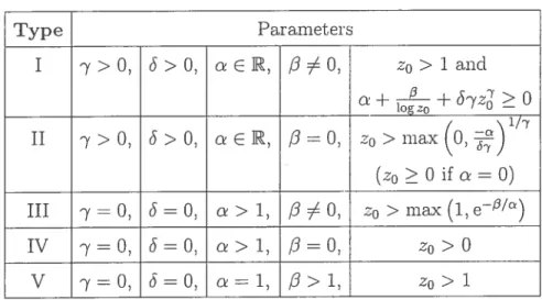
The family of GEP densities which satisfy conditions Cl to C4 cnn 5e divicÏecl
in five subsets as shown in Table 1.1. Each subset is cleterminecÏ by tire tau beha—
viour of the densfty. The riglit tau of a GEP clensity is equÏvalent to a generalizeci gamma cÏensity for type II, it is equivalent to n log-gamma cÏensity for type III,
n Pareto density for type IV and a log-Pareto clensity for type V. Type I corres
ponds to n general case. Note that types III and IV are heavy--tailecl distributions
TAB. 1.1. Five types cf the GEP clensity
Type Paramet.ers
I -y>O, >0, cER, /3O, z0>lancï
cl + +€S7z2 0 1/7 II >0,
>o,
=o,
zo>max(O,)(z > 0 if 0)
III 0, = 0, > 1, 0, zo > ma.x (1, e/)
IV y=O, 6=0, a>1, /=0, z0>0
V 7=0, 6=0, cl=1, >1, z0>1
lVIany known cÏistribritions (see Johnson, Kotz anci Balakrishnan, 1994) are special cases of the CEP density. If the parameters c anci z0 of the CEP clensity of type II are set t.o 0, it. gives the exponential power density (sec Box and Tiao, 1962). In addlition, if the parameter y is set to 2, it gives the normal clensity anci if
tue
pararneter is set to 1, it gives the Laplace density. Furthermore, t.he righttau cf tire GEP density cf type II is eqnivalent to a Weihull ciensitv if cl I
—
a gamma clensity if I and cl < 1, a Rayleigh clensity if 2 anci o = —1
and a Maxwell-Boltzrnann clensity if ‘y = 2 anci cl = —2.
The normalizing coirstant K(’y, 6,cl,3, zo) ancÏ tire Jth moment. cf Z are given in Table 1.2, except for the CEP clensity cf type I, which may be evainateci using Monte Carlo simulatiolls with importance sampling.
Note that in Table 1.2, f(\, a) is the incomplete gamma function clefineci by F(\, a)
=
f
e u’du,
E R. a> O (a> O if,\ > 0). In particular, when a = O ancÏ \ > 0, f(À, 0) is the gamma function anci it is clencteci by F()).
L2.2. Dominance relation using p-credence
The CEP clensity was introcluceci te provicle a henchrnark for tire characteri zation of the tail behavicur cf a clensity. Such a characterization is adclressecl hy the notion cf p-credence, clefined in Angers (2000) as follows t
TAu. 1 .2. Normalizing constant
and
moments of tire GEP clensityNormalizing constant Moments
Type K(7,, ,
/3,
z0) E (Zj3),j
> O F(I.E2±I -7 —6 1—+j t 7 ‘ r f 1— 7 \ — e TT 1 I —6z 1—c .,, 7 e -r r(l—’ -[ 7(5 e/3 z”+- t0 yS 7 .)—+j F(1—/l(a—j—l) Iog‘ i Li—a1 — P(1—j3,(—1)Iogzo)1
+i 1o + (‘)‘]
z1og0zo±/3(1<
a—1)iv
(a-’(
— 1) -— (t3—1)(Ïogo)0 v 2—1+logzo)Definitiori 1. A density
f
on R Ïrct.s p-credence (y,,
ci,/3),
denoted byp-cred(f) = (,, ci, /3), if there ezist constants k, K (O < k < K < œ’) such that for ail z E R
<i — p(z ,à,ci,/3,zo) —
wÏrere p(z7,
,
ci,/3, zo) is givert by eqrtation (1.2.1). We also ‘wrzte p-crecÏ(Z) = (y,,ci,/3) if
tire density of Z iras p-credence (y,, ci, i3).
Tire notion of p-creclence characterizes the tau behaviour of a clensity by
companng it to a GEP clensity. Essentially. this clefinition ensures that f(z) S 0f orcler e_sIzI7z a1og z for large values of z. P-credence is clefineci for clensities
having the sanie behaviour in the left anci right tails, like the symmetric clensities
for example. Note that tire parameter zo isnot listeci as an argument in p-crecÏence since it lias no influence on tire tau behaviour (sec Angers, 2000). By Definition 1,
it is trivial to sec that p-credence of p(z’, ,ci,/3, z0) is
(,
,
ci, /3). It shoulci alsofie noteci that allowing 7 to Le negative woulci provicle no more generality
in
tiretau behaviour of a cÏensity. Furthermore, most of the usuaÏ symmetric cÏensities
on R (such as tire normal, Stuclent’s t, Laplace anci logistic) are covereci hy this clefinition of p-creclence.
Once the tau behaviour 0f clensities has been characterized hy p-credence, a
dominance relation can he established to compare them.
Definition 2. Let
f
and g be any two deusities on R. I’Ve say thatj)
f
dom mates g, denoted byf
>- g, if there exists a constant k > O s’uck that f(z) kg(z), Vz R;ii)
f
is equivalent to g, denoted byf
g, if bothf
- g and g >-f;
iii)f
strictiy dom.inates g, denoted byf
>- g, iff
>‘- g but gf.
Note that if p-crecl(f) = (y, 6,û,/3) then
f
p(.y, 6, û,/3, zo), whereP(17,
6, û, /3,z0) is giveil by equation (1.2.1). The densities are orclereci hy thedominance relation as showri in Proposition 1.
Proposition 1. Let
f
and g be two densities on R such that p-cred(f)‘,6’. û’, f3’) and p-cred(g) = (‘y, 6, û, /3), then
i)
f
g if’y’ , = 6, û’ = û and/3’ = /3;ii)
f
- g if:a) ‘y’ <7
b) 7’ ‘y, 6’ < 6;
c) ‘y’ = ‘y, 6’ = 6, û’ <û;
If
f
g, we say thatf
arici g have tise same p-credence anci we write (‘y’, 6’,û’, /3’)(‘y,
6,û,/3).
Iff
>- g, we say that p-creclence off
is lower thais p-credence of g auJ we write (‘y’, 6’,û’,/3’) <(‘y,
6,û,/3).
Fiually we write(‘y’, 6’, û’,/3’) <
(‘y,
6, û,/3) iff
>— g. Note that p-creclence of the GEP densitiesof types I aisci II is larger tisais that of types III anci IV, these latter mies having
thernselves p-credence larger thari that. of type V.
Here û anci
/3
have heen defineci clifferently from Angers (2000) in orcler toease the comparison of p-credences. In fart, wheo p-crecl(f) = (‘y’, 6’, û’,f3’) and
p-crecl(g)
(‘y,
6, û,/3)
are compared using Proposition 1, the parameters arecompared from left to right. As soon as an inecna1ity between two parameters
occrirs, we say that tue density with the largest parameter has the largest p
1.3. IMPORTANCE SAMPLING
In this section, the estimation of the posterior moments in Bayesian inference wjth location parameter is st.u.diecl. It. is assumeci tliat p-creclence of the prior
anci die likelihood are defineci. The GEP clensity is proposeci as an importance
function when the estimation is performeci using Monte Carlo simulations with importance sampling.
1.3.1. Setting
Consicler n + I clensities f(x — 9), i = O, ..., n, defined on R with j) p-crecl(f) = (‘yj,
,
cj,/3j), i = O,...,
n,ii) the clensity of the data X9 is f(x — 9), i = 1,
...,
n,iii) the prior clensit.y of O is fo(io — O), where co is a known prior location
par ameter.
If the vector composed of the prior location anci the observations is clenotec[
hy x =
(,
x,...,
x), theii forj
N, thej°’
posterior moment is given byR(O3x) = I(x)/Io(x), where
p03 7?
I(x)
J
93 flf(r1— O)dO.
-°°
The algorithrn of IVlonte Carlo for the estimation of E(OJ x) consists in gene rating
••,
9, from an importance function g(O) ancl estirnating I(x) by77?
(x) —Z9w(O,),
7T?. k=1
where the weight function W(Ok) is given hy
9 - fl0f(x-9k)
w( k)
— g(O)
The jtl? posterior moment is then estimated hy (O3x) (x)/(x). Note that any constant can be multiplieci to the weight function silice it cancels ont in the
evaluation of R(&3 Ix).
The choice of g(O) is the main issile of this section. The GEP density with a location pararneter, given hy p(O —
,
c, /3* z), is proposed as an impor tance function. The selection of parameters is acÏdressed in the next subsections.1.3.2. The uniform part of the importance function
The flrst criterion for the choice of tire parameters of the GEP clensity is that the importance function shoulci be close fo tire posterior. Tire posterior density can be multimodal, with possible modes arouncl the prior location anci arounci
each observation. It is thus clifficuit to choose an importance function close to the
posterior. At least, their mass shoulcl be in the same area. This will be adclressecl
hy the uniform part of tire GEP density.
Tire parameters anci z are cirosen to ensure that the rmiforrn part of the
GEP clensity is covering most. of tire prior auJ tire likelihooci (expressecl as a fuirc tion of 9). Let us first clefine tire (loop)th percentile of
f
for i O, ...,n, denotecl by qpj, sucli thatj
f(z) dz p. Tire location parameter of flic importancefunction is then given by
m
-ni2
(1.3.1) wliere
= nrin [ij + qp,j] auJ m2 = max [c +q]_.p,j],
2=0 n 2=0,..., n
airct O < p < 0.5. Furtliennore, to ensure tirat tire uniform part is covering ai least. tue area [m1,rn9], zS must satisfv the condition
ixi2—m1
z . (1.3.2)
In practice, flic choice of p = 0.05 seems appropriate to cover a sufficient
part of flic prior airci tire likehirooci. The ciroice of p heing arbit.rary, a rougir approxilrratioll of the percentiies is sufficient.
1.3.3. Characterization of the posterior using p-credence
Tire second criterion for tire choice of tire paranreters of tire CEP clensity is
that tire importance ftnrctioir ciomiirates tire posterior. This is acÏdresseci witli p
creclence of tire importance function, given by
(,
, «,/3*). These parameters are cirosen 10 nrake p-credence of tire importairce function lower than p-creclenceP-creclence of the posterior clensity with one observation is given in Ai1gers (2000). This resnlt cari be generalizeci to n 1 as follows
p(O — ‘, ‘. ‘. z) where 7’ llIaX7, 6’ —61 [>i], = /‘
t’
e
fl, O < e < z satisftes Conditions Cl, I[[] is the inclicatorfunction of the set {a} and rr(6x) is the posterior clensity under the setup given
in Section 1.3.1.
Choosing the parameters of the importance ftmction such that
(7* *
t3) = (‘. 6’, ‘,‘) (1.3.3)
ensures tliat it clominates the posterior. Then, z cari be chosen in order to satisfy
conditions Cl anci C2 in addition to the condition given by equation (1.3.2), which
gives
= argmin,>1[m2_mi
i±]
(‘
+ + 6’’(z)’ > o) , (1.3.4) where 62 > O. Recali that condition C2 is aiways satisfied if z is large enougli.Note that di anci 62 rniust be specified. In practice, it seems appropriate to
choose di = min (0.01, and 62 = 0.01. A Ïarger value of di world
give an importance function wit.h much heavier tails, which is not necessary. 1.3.4. Simulation of observations from the GEP density
The thirci and Ïast desireci criterion for the choice of the parameters of the CEP clensity consists in being able to simulate observations from the importance
funct.ion. The CEP clen.sity, given hy p(zb’, 6,,3, 20). iS symmetric wit.h respect to the origin arici is u iform between —20 and 20. Hence, if the mass of the uniform
part is clenoteci by q anci given by
TAB. 1.3. Simulation of an observation z from a GEP density on
(zo, oc), (note w U[O, 11)
Type z < 1)
t
‘/7 L1()
III (8< 1) exp Iv 71)c’—1 y exp{--} wwhere K(7, ,c, 3, zo) is the normalizing constant given in Table 1.2, then an
observation must be siinulatecl from (—oc, —z0] with probability from uniform [—zo, zo] with probahility qo anci from (zo, oc) with probability
An observation z is generated from (z0, oc) with the inverse transformation methoci, ciepending on the type of the GEP density as shown in Table 1.3. Note
that F(À)(•) is the ccÏf of a gamina distribution with shape ancÏ scale pararneters respectively equal to À > O and 1, anci F(.) is its inverse ccif. An observation z
from (—oc, —ZD] is generatecl in the same way, except for a change of sign.
There are three cases for which direct simulation with the inverse transforma tion methoci is not possible, that is the GEP clensity of t.ype I, type II with a 1
anci type III with /3 1.
However, it is possible to simulate observations with the rejection methoci (sec Ross, 1997). This algorit.hm generates a value from a proposeci distribution, which is accepteci or rejected accorcling to a probahiÏity baseci on tic ratio of the
density of interest and the proposeci clensity. for more cletails, sec Desgagné anci
Angers (2003).
A proposai for cadi one of these three cases is suggesteci in Table 1.4. Tic
clensities have heen chosen for their balance between simpÏicit.y anci efficiency. They are GEP ciensities, lue fie clensities of interest, anci cliffer from them only
by one or two parameters. Direct simulation of observations from tic proposeci
TAB. 1.4. Proposais when direct simulation fromp(zy. ,
, /3,
zo)is not possible
Type Proposai a GEP density of
**
ï or II
(
1) type II(
< 1) P(Z7, à’ 6zo)’ Z)III (/3 1) type III (/3 < 1): p(zO, O, c, 1 — e, z0)
For the case of the GEP density cf type III when
/3
1, /3 is simply replacedby 1 —
e3,
wheree3
> O. For type II when > 1 and for type I, /3 ïs set to O anci c is replaceci by The objective was to choose a clensity as closeas possible to the clensity of interest, but with heavier tails. A criterion which respects this objective consists in choosing
** . p(z7, à, c,
/3,
zo)3 z0) arg mm sup
z p(zy, à, co, O, zo)
This criterion ensures that the probability cf acceptance in the rejectioll methoci
is maximizeci (see Rohert, 1996). Expllcirly, we have
(1.3.5) arminaoE[F_unin(ia)) A1(7, à, co, 0, zo)(c —
if Π+ <min(1, cv).
inin(1 — e4, ce); otherwise
where e4 > O anci K(y, 0, zo) is the normalizing constant for type II given in
Table 1.2.
In practice, e3 = 0.01 anci e4 = 0.01 seems appropriate. Furthermore, the
minimization cf K’(y, à,cto,O, ZO)( — co) with respect te co has to he cloue
numerically. However it can be shown that this funct.ion is st.rictly convex. Note that the proposed cÏensity eau also be useci as an importance function in
Monte Carlo simulations with importance sarnpling to evaluate the normalizing coistant or the moments cf the CEP clensity oftype I, where no analytic forrnuÏae
1.3.5. Selection of pararneters of the importance function
As mentioneci in Section 1.3.1. the proposed importance function is the GEP
clensity given by p(& 6’, c,
4),
as clefined by equation (1.2.1). Theparameters are determined hy equations (1.3.1), (1.3.3) anci (1.3.4).
1f the importance function is a CEP cierisity for which direct simulation is flot
possible, there are two methocis to hanche it. firstly, observations can be simulated with the rejection methoci, as seen in Section 1.3.4. SecolldÏy, the importance function can be replaceci hy the appropriate clensity as given in Table 1.4. In both
cases observations are generated from the same clensity, but ail the observations
are kept in the second method while some are rejectecÏ in the first one. It is simpler
anci more effective to use the second methoci. More explicitly, the modifications of the importance frinction are as follows
i) if7t> 0, > 0, 0 or > O, > O,>1, then replace a hy Œ*z) and /3* by O,
ii) if 7* = 0 = O, *> 1, tt 1, then replace /3* by 1 — 63,
where is given by equation (1.3.5) and 63 > O. Note that it can 5e
shown that this change affects ileither the unimoclality of the importance function,
nor its dominance on the posterior.
1.4. EXAMPLE 1.4.1. Setting
Suppose that a portfohio manager neecÏs a prechiction on the return of the SSP
500 index for the next clay. He asks five experts for their prechiction on the return as well as a 95% confidence interval on tins precÏiction. The manager want.s t.o
combine tins information with lus prior beliefs using the Bayesian model describeci in Section 1.3.1. Accorcling to this setting, the manager chooses
f(x-6) = T5
(Œz)
for i = 0, 1, ..., 5, where T5() is a Student density wit.h 5 clegrees of freedom, which
deviation of
f
is clenoteci by s, then uj v”ÔJs. The Stuclent density is chosento ensure a robust inference (see Angers, 2000). With standard cleviations equal, the opinion of each source of information lias the same weight.
1.4.2. Data
The collected information for the preclicted ret.urn is x (0, —0.6, 0.3. 0.5.
0.7, 1.0). Note that ail mimbers in this exampie are expressecl in percentages. The
standard clevia.t.ions of t.he predictions, extracteci froni flic confidence intervals
given hy the managers and flic prior, are vectorizeci as s (1, 0.5, 1, 0.25, 0.5, 0.5).
for example, the prior beliefs on the precÏicted return consist in a mean of O anci a standard cleviation of 1. Note that the vector of the scale parameters of
f
is then given hy u = (0.775, 0.387, 0.775, 0.194, 0.387, 0.387).The moments of flic posterior distribution of 9 are estimateci using I\’Ionte Carlo simulations witli importance sampling. Three importance functions, as des
cribeci below, a.re compareci.
1.4.3. The importance functions
The first importance function is flic GEP ciensity given by
—/i17,
*3* z). Its parameters are chosen according to formulae given
in Sections 1.3.2 to 1.3.5. If is easy to show that tue (lOOp)tlt anci (100(1 _pflth
percentiles of
f
are evaÏuat.ed respect.ively as qj —2.OlSuj and qi—p,j = 2.015oif p is set to 0.05. Then it is possible to evaluate m1 = min=0 [x + qp,i]
—1.561, 7n2 rnax=0 [x + qy_p,j] = 1.861 and the location parameter p.
rn1+rn2
= 0.15.
It can lic shown that p-credence of cadi source of information is (0, 0, 6, 0). It is tien easy to show that y = 0, n’ 36 anci 3* 0. Finaily it can
lie verifieci that z m2—rnl = 1.711 satisfies ecfuation (1.3.4). Tic ciensity of
flic importance funct.ion is tien given hy p(9 — 0.1510, 0, 36, 0, 1.711). Tus is a
CEP density of type IV (flic right tau being a Pareto cÏensity) for which direct simulation is possible using tic methocl clescribeci in Section 1.3.1.
25
TAB. 1.5. Standard error anci 95% confidence interval for the esti
mate E(x) after 10,000 simulations, for the first exainple
Importance Standard 95%
function error Ci.
p(9 — 0.150, 0, 36, 0, 1.711) 0.003 0.481 f0 0.493
T(clfrr35, ,u=0.423, a=0. 177) 0.002 0.483 to 0.491
T(clfrrrr5, trr0.423, u=0.141) 0.002 0.483 to 0.491
The two other importance functions are, respect.ively, a Stuclent distribution with 35 anci 5 clegrees of freeclom, both centered at 0.423 with a standard de viation of 0.183 (that is a scale parameter of respectively 0.177 anci 0.141). The
clegrees of freedom are chosen to match p-creclence of the importance function
with respectively that of the posterior and the prior clensity The mean ancÏ stan dard deviation are chosen to match those of the posterior if
where N(.) is the standard normal clensity. In this case, if can be shown that
\fl r I 2
/__,i=ofxi/ si E(8x)
L0(Ï/s) and Var(x) =
1.4.4. Resuits
The posterior mean and standard cleviation are respectively evaluateci to
(9Ix) = 0.487 ancÏ /Var(x) = 0.171. The precliction on t.he return of flic
S&P 500 index for flic next day is then estimateci t.o 0.487% witli an approxi
mative 95% confidence interval of (0.145%, 0.829%). The standard error and the approximative 95% confidence interval for E(&x) estimateci with 10,000 iVionte Carlo simulations are given for each importance finction in Table 1.5. This is a case where no apparent conftict exists between the sources of information. which
explains that the result.s are similar, the t.wo concurrent importance functions having a sliglitly better precision. Next, we consider flic case by permutirg flic
second anci fourth elements (si = 0.25 anci s3 0.5) of the vector of flic stan
TAB. 1.6. Standard error anci 95% confidence iirterval for the esti
mate
(9Ix) after
10,000 simulations, for the second exampleImportance Standard 95%
function error C.I.
p(& — 0.15O. 0, 36, 0, 1.711) 0.004 0.336 t.o 0.352
T(df=35.-0.017,u=0.177) 0.050 0.244 t.o 0.444
T(clfr5, rr-0.017, n0.141) 0.013 0.318 to 0.370
first expert (-0.6) and the other sources of hrformation occurs. The importance functions remain the same ones, except for the Student densities which are now centered at -0.017 instead of 0.423.
The posterior mean is then evalnated to E(8x) 0.344 and the posterior stan dard deviation t.o
/r(6Ix)
0283. The standard error and tire approximative95% confidence interval for E(9x) estirnateci with 10,000 Monte Carlo simula tions are given for each importance frmctions in Table 1.6. (Based on normality assumption, tire intervaÏ corresponds to tire mean plus or mimis two standard errors.) Tins is a case where a confiict exists between tire sources of informa tion. Tire proposecÏ methoci is not affected bv tire confiict.ing information wlren
tire CEP clensity is tire importance ftmction, tire standard error of the estimate
being similar to that of tire first example. Hoever the precision of tire estirnate
is seriously affectecï with tire two concurrent importance functions.
Tire posterior clensit.y as weil as t.he three importance functions are shown in
figures 1(a) anci 1(b) for the two examples. Tire location of tire Studeirt clensities
in tire second example unclerestimates tire location of tire posterior, winch is explaineci by tire influence of tire confiicting information of tire first expert (-0.6).
Tic densit.ies i(ci —9) = T5((r— 9)/uj) are shown for i = O 5 in Figures 1(c)
and 1(d) for tire two examples.
In Figures 2(a) anci 2(b), tire weights (clivided hy their maximum) are plotted over tireir corresponding variates generated iII Monte Carlo simulations, for eadh
importance function and for the two examples. Tire weight.s are expecteci to ire larger and nrore concentrated in tire nrain area of tire posterior. Also tire weights
27 25 2 15 Q —5 —2 —15 —l —05 0 05 I (e) 15 2 (cl) FIG. 1.1. The posterior ancl the importance functions ta) for the
first example, (b) for the second example; the clensities
f
txi — 9)for j 0, ..., 5 te) for the first example, tel) for the second example.
shoiilcl clecrease towards O when the observations move away from the posterior.
These featrires are satisfied when the importance function is the GEP clensity, anci also for the Stuclent density with 5 degrees of freedom except for the mass of
the weights locateci on the right of the posterior in the second exampÏe. However, the Stuclent clensity with 35 degrees of freedom fails to incorporate these even for
the first example.
-;‘l\I D
ta) tb)
o
o
Fia. 1.2. The weights (clivicled by their maximum) over their cor— responchng observation for each importance ftmction (a) for the first example (b) for tire second example.
(a)
1.5. CoNcLusioN
Tire generahzed exponential power density iras been proposeci as an impor
tance function in Monte Caria simulations in tire coutext of tire estimation of posterior moments of a location parameter. It can 5e clifficuit. to choose an appro priate importance function anci it must often 5e clone for eacir case. If p-creclences
of tire prior ancÏ tire likelihooci are clefineci, tire parameters of tire GEP clensity
are obtainecl by tire equations given in tins paper, in an automatic wa.y wiratever
tire moclel anci tire data are. Note tirat p-creclence is ciefineci for most of tire usual
symmetric distributions clefineci oir tire real une witir air exponential, polynomial
or logaritirmic beiraviour in tireir tails.
Tire ciroice of tire GEP clensity aliows us to obtain rehabie results, even if tirere
are conflicting sources of information. Furtirermore, since p-credeuce of tire GEP
clensity is sligirtÏy iower than tirat. of tire post.erior, tire Monte Carlo simulations
renraiir effective as iilustratecl in Section 1.4. Tire simulation of observations from
tire GEP density iras been adclressecl with tire inverse transformation nrethocl.
1.6. ACKN0WLEDGMENTS
Tire autirors are thankfuÏ ta the NSERC (Natural Sciences anci Engineering
Researcir Council of Canada), tire FQRNT (Le Fonds québécois de la recirerche sur ia nature et les technologies) anci tire SOA ($ociety of Actuaries) for their financiai support. Tirey also wouÏcl like to tirank tire referees, Prof. Yogeirdra Chaubey
anci James IVierleau for tireir useful conrnrents winch irave brouglit substantial
improvements air a previous draft.
1.7. REFERENCES
ANGERS, J-F. (1992) Use of Shtdent-tpriorforthe estiriration ofn,ornraÏrneans:
A computational appioach, Bayesian Stalistic IV ecis. Bernardo, J. M.., Berger,
J.O., David, A.P., and Srnith, A.F.M., New York Oxford University Press, pp.
567-575.
ANGERS, J.-F. (1996) Protection agaiirst outhers using a symnretric stable iaw
ANGERS, J-f. (2000) P-Credence and outiiers, Metron, 58, 81-108.
ANGERS, J.-F. auJ BERGER, J.O. (1991) Robust hierarchical Bayes estimation
of exchangeable means, The Canadien Journal of Statistics, 19, 39-56.
BOX, G. a.ncl TIAO, G. (1962) A ftirther look at robustness via Bayes’s theorem,
Biometriha, 49, 419-432.
CARLIN, B. anct POLSON, N. (1991) Inference for nonconjugate Bayesian mo
ciels using the Gibbs sampler, The Canadien Journal of $tatistics, 19, 399-405.
DESGAGNÉ, A. anci ANGERS, J.-f. (2003) Computational aspect of the 9e-neralized exponential power density, Technical report CRM-2918, Université de Montréal (http //www. crm.urnontreal. ca/pub/Rapports/2900-2999/29 18 .pdf).
FAN, T.H. anci BERGER, J.O. (1992) Behaviour of the posterior distribution and inferences for a normal means with t prior distributions, Statistics & Decisions,
10, 99-120.
GEWEKE, J. (1994) Priors for macroeconomic time series auJ their applications, Econometric Theory, 10, 609-632.
JOHNSON, N.L., KOTZ, S. AND BALAKRISHNAN, N. (1994) Continuons uni variate distributions, Vol. 1 (second edit.ion), Wiley, New York.
MEINHOLD, R. anci SINGPURWALLA, N. (1989) Robustification of Kalman ifiter moclels, Journal 0f the American Statistical Association. 84, 479-486.
O’HAGAN, A. (1990) Outiiers anci creclence for location parameter iiference,
Journal of the American Statistical Association, 85, 172-176.
REISS, R.-D. ancl THOMAS, M. (1997) Statistical analysis oJ extreme values,
Birkhauser Verlag, Basel.
ROBERT, C. (1996) Méthodes de Monte Carlo par chaînes de Markov, Econo
mica, Paris.
OUTLIER$ AND CHOICE 0F THE PRIOR
FOR LOCATION PARAMETER INFERENCE
Cet article a été soumis pour publication en février 2005 clans la revue Metron. Le premier auteur est Alain Desgagné et le coauteur est le directeur de recherche Jean-françois Angers. La contribution de Alain Desgagné à cet article consiste en la conception. recherche, développement, progranimation informatique et. rédac tion de toutes les parties de l’article, sous la supervision clii directeur de recherche.
Abstract
The use of heavy-tailecl distributions is a valuable tool in developing robust Baye sian procedures. limiting the influence of outiiers on posterior inference. In this paper, the hehavior of the posterior clensity of the location parameter is investiga teci when the sample contains outliers. The notion of left and right p-creclence is introcluceci to characterize respectively the left ancl right tail of a densit.y. Simple conditions on the t.ails of the prior anci the likelihood, using left anci right p creclence, are estahiisheci to cletermine the proportion of observations that can be rejected as outliers. It is shown that the post.erior distribution converges in law to the posterior tl;at woulcl be ohtained from tire recluced sample, exciuding t.he outiiers, as they tend to plus or minus infinity, at any giveil rate. An example of combination of preclictions of the S&iP 500 index return is presented.
Key words Baesian inference, Outiier, Heavy-tailed modeling, Ceneralizecl exponential power family, Location pararneter.