A shape optimization formulation of weld pool determination

(1)

HAL Id: hal-00678430

https://hal.archives-ouvertes.fr/hal-00678430

Submitted on 12 Mar 2012

HAL is a multi-disciplinary open access

archive for the deposit and dissemination of

sci-entific research documents, whether they are

pub-lished or not. The documents may come from

teaching and research institutions in France or

abroad, or from public or private research centers.

L’archive ouverte pluridisciplinaire HAL, est

destinée au dépôt et à la diffusion de documents

scientifiques de niveau recherche, publiés ou non,

émanant des établissements d’enseignement et de

recherche français ou étrangers, des laboratoires

publics ou privés.

A shape optimization formulation of weld pool

determination

Abdelkrim Chakib, Abdellatif Ellabib, Abdeljalil Nachaoui, Mourad Nachaoui

To cite this version:

Abdelkrim Chakib, Abdellatif Ellabib, Abdeljalil Nachaoui, Mourad Nachaoui. A shape optimization

formulation of weld pool determination. Applied Mathematics Letters, Elsevier, 2011, 25 (3),

pp.374-379. �10.1016/j.aml.2011.09.017�. �hal-00678430�

(2)

A shape optimization formulation of weld pool determination.

A. Chakiba_{, A. Ellabib}b_{, A. Nachaoui}c_{, M. Nachaoui}a,c

a_{Laboratoire de Mathématiques et Applications Université Sultan Moulay slimane, Faculté des Sciences et Techniques, B.P.523, Béni-Mellal,}

Maroc.

b_{Université Cadi Ayyad, Faculté des Sciences et Techniques, B.P 549, Guéliz Marrakech, Maroc.}

c_{CNRS UMR6629, Universit´e de Nantes, BP 92208, 44322 Nantes, France.}

Abstract

In this paper, we propose a shape optimization formulation for a problem modeling a process of welding. We show the existence of an optimal solution. The finite element method is used for the discretization of the problem. The discrete problem is solved by an identification technique using a parameterization of the weld pool by B´ezier curves and Genetic algorithms.

Keywords: Welding, Shape optimization, Non coercive operator, B´ezier curves, Genetic Algorithms.

1. Introduction

The determination of temperature field in a welding process permits the control of mechanical effects (residual stress, distortions, fatigue strength...). Many models are proposed in literature [1, 6].

The approach used here deals only with the solid part of the workpiece. It consists to simplify the physical phe-nomenon appeared between the welding torch, the workpiece and the liquid pool, by considering that the temperature field on the interface liquid/solid Γ is known.

In the shape optimization formulation that we propose, it appears a state problem governed by a non-coercive equation. This complicates the study of the existence of an optimal solution and more precisely, the uniform extension of the solution of the state problem with respect to domain.

We show the existence of an optimal solution by using recent results on uniform Poincarr´e inequality [2], and some Sobolev inequality [9], this is reported in section 3. Some numerical results are given in the last section showing the efficiency of our approach.

The welding problem consists in finding Γ the weld pool and T the temperature gradient in the workpiece, solution

of: _                               K∂T ∂x = ∇ · (λ∇T ) + f in Ω λ∂T ∂ν = 0 on Γ0∪ Γ1∪ Γ2∪ Γ3 T = Td on Γ4, T = T0 on Γ0 T = Tf on Γ (1)

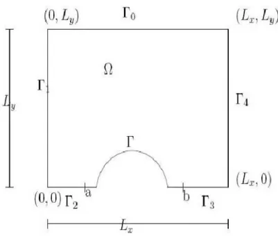
where Ω denotes the solid part of welded workpiece (see Fig 1); K is a function depending on the density of the Email addresses: [email protected] ( A. Chakib), [email protected] ( A. Ellabib),

(3)

Figure 1:The solid part of the welded workpiece with interface Γ.

material and the heat capacity and independent of T ; λ is the thermal conductivity; f is a given source term. The quantities Td, T0and Tf are the given temperatures.

In the sequel we suppose that the parameters of our problem are such that: Let D =]0, Lx[×]0, Ly[,

(H1) λ ∈ L∞(D) and ∃λ0> 0 such that λ(x)ξ · ξ ≥ λ0|ξ|2p.p x ∈ D

(H2) K ∈ L∞(D)

(H3) f ∈ L∞(D)

2. The shape Optimization Formulation

The shape optimization formulation of problem (1) that we propose is given by:                                                    find Ω∗_{∈ Θ} ad solution of J(Ω∗_{) = inf} Ω∈Θad J(Ω) where J(Ω) = 1 2 R Γ0|TΩ(x, y) − T0| 2_dσ

and TΩis the solution of

(PE)                          K∂T_∂x = ∇ · (λ∇T ) + f in Ω λ∂T_∂ν = 0 on Γ0∪ Γ1∪ Γ2∪ Γ3 T = Tdon Γ4, T = Tf on Γ (2)

where the set of admissible domains Θad is defined by

Θad = {Ω(ϕ) / ϕ ∈ Uad}

(4)

with Ω(ϕ) =]0, a[×]0, Ly[∪ n (x, y) ∈ R2/a ≤ x ≤ b, ϕ(x) ≤ y ≤ Ly o ∪]b, Lx[×]0, Ly[ and Uad = n

ϕ ∈ C([a, b]) / ∃aϕet bϕ, ϕ|[a,aϕ] = 0 , ϕ|[bϕ,b] = 0 and

ϕ(x) − ϕ(x0₎_{≤ C}

0x − x0 ∀x, x0∈ [a, b] , 0 ≤ ϕ(x) ≤ Ly∀x ∈ [a, b]

o where C0is the uniform Lipschitz constant.

In the next section we study the existence of a solution to problem (2). 3. Existence of the optimal solution

From the surjectivity of the trace operator from H1_{(D) to H}1 2(∂D), ∃ V ∈ H1_(D) _{such that} _{V =}              v on ]b, Lx[×]0, Ly[ Tf on ]0, b[×]0, Ly[, where v ∈ H1_{(]b, L}

x[×]0, Ly[) such that v = Tdon Γ4and v = Tfon {b} × [0, Ly] .

Let ΓD= Γ ∪ Γ4, we define the following Sobolev space H_Γ1_D(Ω) =

n

u ∈ H1_{(Ω) / u|} ΓD = 0

o

, and take u = T − V, then we consider the weak formulation:

               find u ∈ H1 ΓD(Ω), Z Ω λ∇u · ∇ψdxdy + Z Ω K ψ∂u ∂xdxdy = hL, ψi((HΓD1 (Ω))0,HΓD1 (Ω)) ∀ψ ∈ H 1 ΓD(Ω), (3)

where L is the operator defined by, hL, ψi_((H1 ΓD(Ω))0,HΓD1 (Ω)) = Z Ω f ψdxdy − Z Ω λ∇V · ∇ψdxdy − Z Ω K ψ∂V ∂xdxdy.

Remark 1. Note that according to the assumptions (H1) − (H3), we have L ∈ (H_Γ1_D(D))0and that there exists δ > 0 such that kLk(H1

ΓD(Ω))0≤ δ ∀Ω ∈ Θad.

Define the space F

F = {(Ω, u(Ω)) | Ω ∈ Θad and u(Ω) solution of (3) in Ω}. (4)

and consider the following shape optimization problem

Minimize J(Ω, u(Ω)) for all (Ω, u(Ω)) ∈ F . (5)

Note that T = u + V is solution of (PE) for each u solution of (3). Thus if (Ω, u(Ω)) is solution of (5) then (Ω, T (Ω)) is solution of the problem (2).

The existence of an optimal solution of (5), requires the definition of a topology on F , which ensure the compact-ness of F and the Lower semicontinuity of J on F .

For this, let Ωn= Ω(ϕn), Ω = Ω(ϕ), un= u(Ωn) and u = u(Ω), and define the convergence of Ωnto Ω by

(5)

Then we consider on F the topology defined by the following convergence: (Ωn, u(Ωn)) −→ (Ω, u(Ω)) ⇐⇒        Ωn−→ Ω

˜un* ˜u weakly in H1(D) when n −→ ∞,

(7) where ˜u is a uniform extension in H1_{(D) of u ∈ H}1_{(Ω) (see D.Chenais [3]).}

Then we have the following result

Theorem 1. Under the assumptions (H1) − (H3), the problem (5) is well posed and admits at least one solution in F

The proof of this theorem is based on the following lemmas.

Lemma 1. Under assumptions (H1) − (H3), the state problem (3) admits a unique solution.

The presence of the term ∂T_∂x in the state problem equation, does not allow to have the coercivity, which is necessary for the application of the classical result of Lax-Milgram, without restriction on the physical parameters of the prob-lem (K and λ ). To overcome this probprob-lem, we use Leray Schauder topological degree [4]. To show this prob-lemma, we consider the following application:

G : H1

ΓD(Ω) 7→ H

1 ΓD(Ω)

¯u 7→ u

where u is the unique solution of problem: Z

Ω

λ∇u · ∇ψdxdy = hL, ψi((H1

ΓD(Ω))0,HΓD1 (Ω))− Z Ω K ψ∂¯u ∂xdxdy ∀ψ ∈ H 1 ΓD(Ω). (8)

It’s easy to see that G is well defined. Remark 2. Note that for all ¯u ∈ H1

ΓD(Ω), the existence of the unique solution of the problem (8) is obtained thanks to

the Lax-Milgram result.

A fixed point of G is solution of (3). To prove the existence of fixed point of G, we have to show that G is compact and continuous, and find R > 0 such that ∀t ∈ [0, 1], there exists no solution of u − tG(u) = 0 satisfying kuk1,Ω = R.

For the compactness of G it suffices to show, using ψ = G(¯un) = ¯unas a test function in (3), that if (¯un)nis bounded in

H1

ΓD(Ω) then (un)nis a Cauchy sequence in H

1

ΓD(Ω) and converges in this space. It’s easy to see that G is continuous.

For the last point we show that there exists C > 0 such that kuk1,Ω< C then we take R = C + 1.

For the uniqueness of the solution, since (3) is a linear problem, we show that the only solution of (3) with L = 0 is the null one.

The compactness of F for the topology defined in (7) requires the compactness of Θad, which follows from the

Ascoli Arzel`a theorem, and the continuity of the state problem based on the following lemmas.

Lemma 2. Under the assumptions (H1)−(H3), we have: for all u ∈ HΓ1D(Ω) solution of (3) in Ω, there exists a uniform

extension ˜u ∈ H1_{(D) of u and M > 0 independent of Ω ∈ Θ}

adsuch that:

k˜uk1,D≤ M. (9)

Proof

Note that the uniform cone property [3] is satisfied for all Ω in Θad, thus for all u ∈ H1_Γ_D(Ω), there exists ˜u ∈ H_Γ1_D(D)

and a constant c > 0 independent of Ω such that k˜uk1,D≤ c kuk1,Ω.

(6)

The main difficulty of this work is to show that kuk1,Ωis uniformly bounded with respect to Ω. For this we use the

two following inequalities (see [2, 9])

- There exists C0> 0 independent of Ω such that ∀u ∈ H_Γ1_D(Ω) C0kuk2_H1_(Ω)≤

Z

Ω

|∇u|2dxdy. (10)

- There exists C > 0 independent of Ω such that

kukL4_(Ω)≤ C|Ω| 1

4kuk_H1_(Ω). (11)

Then we define the set Ak= {x ∈ Ω, |u(x)| > k} and the functions hk(u) = max(−k, min(u, k)) and ψk(u) = u − hk(u).

First we show the following uniform estimation of ψk(u):

(C0− C|Ak| 1

4) kψ_k(u)k2

H1_(Ω)≤ | < L, ψk(u) >((H1

ΓD(Ω))0,H1ΓD(Ω))| (12)

To show that the constante (C0− C|Ak| 1

4) is positive, we use an idea of Droniou and Gallouet [5]. We start by showing

the uniform control of Lebesgue measure of Ak, using Tchebycheff inquality and the uniform estimate of ln(1 + |u|),

i.e. there exists C2> 0 independent of Ω such that

|Ak| = |{(x, y) ∈ Ω/ ln(1 + |w|)2≥ ln(1 + k)2}| ≤ 1

ln(1 + k)2kln(1 + |w|)kL2(Ω)≤ C2

ln(1 + k)2 (13)

Then there exists k0∈ N∗, such that

∀k ≥ k0 C|Ak|

1 4 ≤C0

2 . (14)

Taking k = k0, we show that there exists C3> 0 independent of Ω such that

ψk0(u) _H1_(Ω)≤ C3. (15)

Finally, using the fact that hk0(u)u ≥ (hk0(u))2, ∇hk0(u) = χA_k0∇u and the inequality (10), we show that there exists

C4> 0 independent of Ω such that

hk0(u) _H1_(Ω)≤ C4. (16)

To conclude, we show this result:

Lemma 3. (i) Let un∈ H1ΓD(Ωn) be the solution of (3) on Ωn, there exists ˜una uniform extension of unwhich converges

weakly in H1_{(D) to a limit denoted W, such that u = W|Ω}∗_{is the solution of (3) in Ω}∗_{, where Ω}∗_{is the limit of Ω}

nfor

the topology defined by (6).

(ii) The cost functional J is lower semicontinuous on F . Proof

(i) Using the Lemma 2, for a sequence (un)n, such that un∈ HΓ1D(Ωn), we can extract a subsequence of (˜un)n, where

˜un is the uniform extension of un, which converges weakly to W in H1(D). To show that u = W|Ω∗ is solution of

equation (3) on Ω∗_{, it’s easy to see that u|}

Γ4 = 0 and according to the compactness of the trace operator from H

1_(D)

into L2_(Γ∗_{), we show that u ∈ H}1

ΓD(Ω∗). Now, it suffices to show that u is solution of the weak formulation of the

equation (3) on Ω∗_{. Indeed, let ψ ∈ H}1 ΓD(Ω

∗_{), and denoted by ˜ψ ∈ H}1_{(D) an extension of ψ defined by}

˜ψ =        ψ in Ω 0 in D \ Ω.

(7)

Then we can construct a sequence (ψj)j, ψj∈ D( ¯D), such that,

dist(supp ψj, ΓD) > 0 ∀ j ∈ N and ψj→ ˜ψ in H1(D), j → ∞.

Let j ∈ N, since Ωn→ Ω∗, there exists n0such that ψj|Ωn∈ H

1

ΓD(Ωn), ∀n ≥ n0.

For all n ≥ n0, we have

Z D χ_Ωnλ∇˜un· ∇ψjdxdy + Z D K χ_Ωnψj∂˜un ∂xdxdy = hL, χΩnψji((H_ΓD1 (Ω))0,H_ΓD1 (Ω)) (17)

Using the convergence of characteristic functions χΩnto χΩ∗in L

2_{(D), the weak convergence of ˜u}

nto ˜u in H1(D), the

convergence of ψj to ˜ψ in H1(D) and by passing to the limit in equation (17), we obtain that u solution of a weak

formulation (3) in Ω∗_.

(ii) The continuity of J on F is based on the weak convergence of ˜unto ˜u in H1(D) and the compactness of the

trace operator from H1_{(D) into L}2_(Γ 0).

4. Numerical results

The shape optimization problem is approached by the P1finite element method. The free boundary is

parameter-ized by piecewise spline approximation locally realparameter-ized by quadratic B´ezier functions. These allow to have a smooth domains and in the same time they are defined by a finite number of parameters. The corresponding discrete prob-lem is solved by the genetic algorithms. Genetic algorithms (GA), primarily developed by Holland [8], have been successfully applied to various optimizations problems. It is essentially a searching method based on the Darwinian principles of biological evolution. It offer a good robustness, since they do not impose any regularity requirements on objective functions. Moreover, as (GA) are global optimization methods they can find new innovative designs instead of traditional designs corresponding to local minima. The GA is summarized in the following algorithm see [10].

begin

t ← 0

initialize a population P(t) evaluate P(t)

while (not termination-condition) do begin t ← t + 1 select P(t) from P(t − 1) alter P(t) evaluate P(t) end end

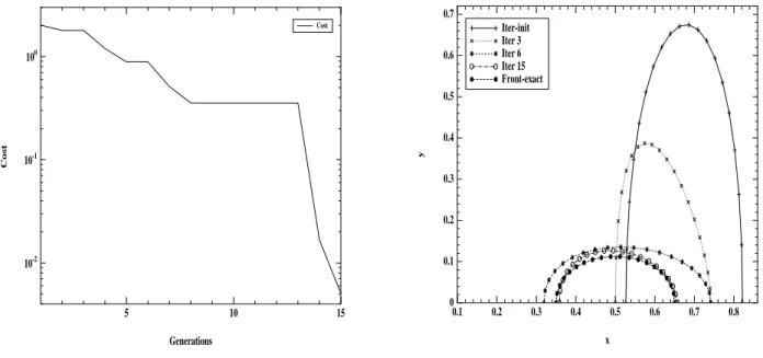
To test the efficiency of our algorithm, we present an approximation of the exact solution u = exp(x + y) and the exact boundary Γ parameterized by the half circle with center (0.5, 0.0) and radius r = 0.15 (for Lx= 1, Ly= 1, K = 1 and λ = 1).

(8)

The following figures show that the cost decreases with respect to the number of iterations. The obtained numerical results are found to be in good agreement with the exact solution.

x y 0.1 0.2 0.3 0.4 0.5 0.6 0.7 0.8 0 0.1 0.2 0.3 0.4 0.5 0.6 0.7 Iter-init Iter 3 Iter 6 Iter 15 Front-exact Generations Cost 10 5 15 -2 10 -1 10 0 10 Cost

Figure 2: Cost functional and boundary evolution

Acknowledgment

Supported in part by Convention CNRS/CNRST 21585 and AI-Volubilis MA/09/202 References

[1] Bergheau,J. M. Numerical simulation of welding, Revue européenne des éléments finis, volume 13 no 3-4, 2004.

[2] Boulkhemair, A.; Chakib, A. On the uniform Poincar´e inequality. Comm. Partial Differential Equations 32 (2007), no. 7-9, 1439–1447. [3] Chenais, D. (1975), On the Exitence of a Solution in a Domain Identification Problem, J. Mat. Annal. Appl. vol.52, No_{2, pp. 189-289.}

[4] Deimling, D. Nonlinear Functional analysis, Sprenger,1985.

[5] Droniou J.; Gallouet, T. A uniquness result for quiasilinear elliptic equations with mesures as data. Rend. Mat. Appl. (7)21(2001), no. 1-4, 57–86

[6] Feulvarch, E.; Boitout, F.; Bergheau, J. Simulation thermom´ecanique du soudage par friction-malaxage, European Journal of Computa-tional Mechanics, Vol 16/6-7 - 2007 - pp.865-887

[7] Haslinger, J.; Makinen, R. A. E. Introduction to shape optimization. Theory, approximation, and computation. Advances in Design and Control, 7. SIAM, Philadelphia, 2003.

[8] Holland, J. Adaptation in natural and artificial systems University of Michigan Press, Ann Arbor, Mich., 1975.

[9] Ladyzenskaja,O.A; Ural’ceva,N.N : Équations aux Dérivés Partiales de type elliptiques, Monographies universitaires de Mathématiques, Dunod Paris 1968.