HAL Id: hal-02191501
https://hal-lara.archives-ouvertes.fr/hal-02191501
Submitted on 23 Jul 2019
HAL is a multi-disciplinary open access
archive for the deposit and dissemination of
sci-entific research documents, whether they are
pub-lished or not. The documents may come from
teaching and research institutions in France or
abroad, or from public or private research centers.
L’archive ouverte pluridisciplinaire HAL, est
destinée au dépôt et à la diffusion de documents
scientifiques de niveau recherche, publiés ou non,
émanant des établissements d’enseignement et de
recherche français ou étrangers, des laboratoires
publics ou privés.
Project porcupine : the MF mutual-impedance probe
experiment. Part II : Flight F3 and F4 (March 1979)
L.R.O. Storey, J. Thiel, J.M. Illiano
To cite this version:
L.R.O. Storey, J. Thiel, J.M. Illiano. Project porcupine : the MF mutual-impedance probe experiment.
Part II : Flight F3 and F4 (March 1979). [Rapport de recherche] Centre de recherches en physique de
l’environnement terrestre et planétaire (CRPE). 1981, 194 p., figures, graphiques. �hal-02191501�
CENTRE NATIONAL D'ETUDES DES TELECOMMUNICATIONS
CENTRE NATIONAL DE LA RECHERCHE SCIENTIFIQUE
CENTRE DE RECHERCHES EN PHYSIQUE DE
L'ENVIRONNEMENT TERRESTRE ET PLANETAIRE
NOTE TECHNIQUE CRPE/94
PROJECT PORCUPINE
THE MF MUTUAL-IMPEDANCE PROBE EXPERIMENT
PART 2 : - FLIGHTS F3 and F4 (MARCH 1979)
By
L.R.O. STOREY, J. THIEL, and J.M. ILLIANO
C.R.P.E./R.P.E.
45045 ORLEANS CEDEX
CONTENTS
PART 2 :- FLIGHTS F3 and F4 (MARCH 1979)
6. PREFACE 7. INSTRUMENTAL MODIFICATIONS 7.1. MF Sensor 7.2. Electronics 7.3. Other instruments 8. PORCUPINE F3 8.1. Technical aspects 8.1.1. Calibrations 8.1.2. Sensor system 8.1.3. Passive mode 8.1.4. Active mode 8.2. Scientific results 8.2.1. Frequency-shifts 8.2.2. Spin-dependence 8.2.3. Amplitude-shifts 8.3. Discussion
8.3.1. Summary of probe performance 8.3.2. Reduction of random errors 8.3.3. Evidence of systematic errors
9. PORCUPINE F4 9.1. Technical aspects 9.1.1. Calibrations 9.1.2. Sensor system 9.1.3. Passive mode 9.1.4. Active mode
II
9.2. Scientific results 9.2.1. Frequency-shifts 9.2.2. Spin-dependence 9.2.3. Amplitude-shifts 9.3. Discussion9.3.1. Summary of probe performance 9.3.2. Causes of systematic errors 9.3.3. Reduction of systematic errors
10. CONCLUSIONS ACKNOWLEDGEMENTS REFERENCES FIGURE CAPTIONS FIGURES TABLE CAPTIONS TABLES
6. PREFACE
This is the second part of a report on the results from the medium-frequency (MF) mutual-impedance probe experiment that was supplied by the Centre for Research in Environmental Physics (CRPE, Orléans,
France) as a contribution to the West-German Porcupine program of research on auroral physics during the International Magnetospheric Study.
The subject of Part 1 was the results from the first successful flight, named F2, which took place from ESRANGE (Kiruna, Sweden) on 20 March 1977. On that occasion, the MF probe experiment did not succeed in its objective of detecting field-aligned drift motion of the thermal electrons in the auroral ionosphere. The non-reciprocal shift of the lower oblique resonance (L.O.R.) frequency that this motion should have produced was masked by a similar but much larger shift that was obviously
spurious, since it varied, more or less sinusoidally, as a function of the spin-phase angle. Various conceivable physical causes for this spurious shift were studied, but were rejected. The question of whether the true cause was some other physical phenomenon, as yet unidentified, or whether it was technological in nature, had to be left open. The results from the flight F2 nevertheless suggested a number of ways in which the experi- ment could be improved, and these were discussed in Section 5, which
concluded Part 1 of the report.
In Part 2, after the present preface, Section 7 describes how these and other modifications were made to the MF probe, in preparation for the flights F3 and F4. The changes that were made to some of the other instruments on board are mentioned also.
The flight F3 took place on the evening of 19 March 1979, during a quiet interval within a period of repeated auroral activity. A weak negative magnetic bay of about 100 y (K = 2 ) was in progress at the time of launch : see § 7.2. of the report by H�1U�2A � 0�. [1982] . The aurora failed to evolve as anticipated, and the payload did not pass through any discrete arc. These relatively calm conditions, which disap- pointed the other experimenters, were ideal for determining whether
- 98 -
the various modifications had improved the MF probe. In Section 8, where the results of the F3 experiment are presented, emphasis is therefore laid on analysis of the technical performance of the probe.
The flight F4, on the evening of 31 March 1979, took place during a strong magnetic substorm
( p = 5+). At the time of launch,
a dis- crete visual arc was present with a sharp northern edge, and the trajec- tory of the payload crossed this edge ; see § 7.3. of the report by H�i,6£-eA P.t 0�..
[1982] . Stronger electric fields were encountered on this flight than on F3, and much of our study of the experimental results in Section 9 has been devoted to clarifying certain effects that appear to have been caused by these fields, and which resemble the spurious ef- fects already observed on F2 inasmuch as they depended on spin phase and masked the interesting effects that we were looking for.
The conclusions, presented in Section 10, are drawn from the results of all three successful flights. They substantiate the progress made in the development of the MF mutual-impedance probe as a means for measuring the field-aligned drift velocity of the thermal electrons,
and indicate how, by further development, it might be made into a reliable instrument for this purpose.
7. INSTRUMENTAL MODIFICATIONS
7.1. MF SENSOR
In Section 5, a discussion of the results from the flight F2 led to several suggestions for improvements in the design of the MF sen- sor, which may be summarized as follows :
- that the double-monopole layout of the sensor units be
adopted definitively, to the exclusion of the various quadripole layouts ;
- that the spin axis of the payload be aligned with the Earth's magnetic field, instead of being set at an angle of 30° to the field ;
- that one of the telescopic booms that support the two sensor units be made longer than the other, in order that the sensor axis (i.e. the line joining the centres of the two electrodes) may still be inclined at about 30° to the field.
Together, these modifications led to the design of double-monopole sensor illustrated in Figure 20 (see Part 1). �
The particular dimensions shown in the figure were chosen so as to minimize the mechanical changes that would be required. Thus the spacing of the two booms along the payload axis, and also the length of one of them, were the same as on F2. The sole mechanical change was the lengthening of the other boom by 0.5 m.
On F2 there were four boom-mounted sensor units, and the de- cision was taken to have the same number on each of the F3 and F4 payloads, though this was not strictly necessary. The main reason for this choice was to insure against the risk of failure either of a boom or of a sensor unit, such as occurred on F2 and plagued the interpretation of the data. With four booms spaced uniformly along the payload axis, it is possible to compose a sensor of the type shown in Figure 20 in three possible ways, one for each pair of adjacent sensor units. The requirement that adjacent units be on booms of different lengths led finally to the design illustrated in Figure 21.
- 100 -
In comparison with the arrangement on F2, on the flights F3 and F4 the four booms were turned through 45° around the payload axis so as to increase the distances between the sensor units and the payload base. in the hope of reducing interference from the telemetry system.
Because of the higher degree of symmetry that this new system possesses, it should be unaffected by most of the possible causes of the spurious L.O.R. frequency-shifts that were observed on F2, and have been discussed in § 4.3. Specifically, it should be immune to the effects of the perturbation of the supra-thermal electron population by the payload body (§ 4.3.2.), to electromagnetic effects (§ 4.3.3.), and to certain technological defects (§4.3.4.). Only the perturbation of the thermal plasma may still produce spurious frequency-shifts.
Moreover, one merit of a sensor system of this type is that if ever the mode of origin of an observed L.O.R. frequency-shift is un- certain, it may be identifiable by comparison of the data from two adja- cent pairs of units. The comparison concerns the dependence of the frequency- shift upon the spin-phase angle,and before discussing it, we must first define these two quantities unambiguously.
As regards the frequency-shift, the only point at issue is its sign. This was defined in § 4.2., and we now recall the definition : the shift Af is counted as positive if the L.O.R frequency is higher when the direction of transmission is towards the base of the payload, than when it is towards the tip.
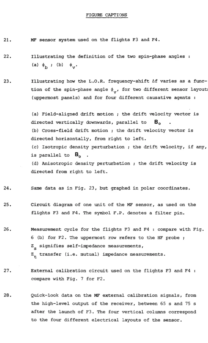
For the spin-phase angle, however, we must now adopt a defini- tion different from the one used in Part 1. The old and the new definitions are compared in Figure 22. In the old definition, the origin of the spin- phase angle 0 was taken as the projection of the magnetic-field vector Bo into the plane perpendicular to the payload spin axis (Fig. 22 a). The angle so defined will henceforth be called
�b. It is not useful for the study of the data from the flights F3 and F4, during each of which the spin axis was almost parallel to Bo , because in these circumstances a small change in the direction of this axis in space could lead to a large change in
�b. Accordingly we now prefer to take the origin of the spin- phase angle to be the projection of the cross-field plasma drift velocity
the theoretical direction of the plasma wake of the payload. With this new definition, the spin-phase angle will be called V .
By comparing the variations of Af versus �vi measured on two adjacent pairs of sensor units, it may be possible to identify any of the following four causes of L.O.R. frequency-shifts :
(a) Field-aligned drift motion, (b) Cross-field drift motion, (c) Isotropic density perturbation, (d) Anisotropic density perturbation.
How (a) and (b) give rise to frequency-shifts was explained in § 2.1. From our point of view, such shifts are genuine, while those caused by (c) or
(d) are spurious. The shapes of the corresponding functions Af(� v) are indicated in Fig. 23, and will now be commented on briefly.
a) Field aligned drift motion
Frequency-shifts due to field-aligned drift motion of the ther- mal electrons should be independent of spin phase, and should have the
same sign on adjacent pairs of units.
b) Cross-field drift motion
In contrast, the frequency-shifts due to cross-field drift motion of the thermal plasma should vary sinusoidally as a function of
spin phase, with an average value of zero, and should have opposite signs on adjacent pairs of units.
c) Isotropic density perturbation
The perturbation of the thermal plasma by the payload body was discussed in § 4.3.1. When the drift velocity of the plasma is zero, or when it is parallel to the axis of the payload, the perturbation is isotropic in the sense that it is independent of azimuth at a given
radial distance from the axis. It can affect a sensor system of the type shown in Fig. 21, because the plasma is more severely perturbed near the sensor unit on the end of the short boom than it is near the unit on the end of the long boom. Accordingly the resultant frequency-shift should be independent of spin phase, but opposite in sign on adjacent pairs of units.
- 102 -
(d) Anisotropic density perturbation
When the drift velocity of the plasma relative to the payload body has a non-zero cross-field component , the plasma perturbation is anisotropic : the reduction of plasma density is greatest in the wake. In this case, therefore, the frequency-shift should vary with spin phase, though without changing sign, which distinguishes it from shifts due to
(b). As with (c), the sign is opposite on adjacent pairs of units. At low cross-field drift velocities the variation might be more or less sinusoidal, though with non-zero mean value, but at large velocities, giving rise to a well-defined wake, it would be markedly non-sinusoidal as is shown in the figure.
Of course, paragraphs (c) and (d) presuppose a mechanism whereby changes in the density of the thermal plasma, greater near one of the sen- sor units of a pair than near the other, can give rise to non-reciprocal L.O.R. frequency-shifts. The possible nature of this mechanism will be considered in § 9.3.2.
The features illustrated in Fig. 23 allow any of the four causes of frequency-shifts to be identified, whenever it occurs on its own. This is not always possible, however. For instance, the effect (d) is inevitably accompanied by (b), which means that they are difficult to distinguish from one another. On the other hand, when the genuine effects (a) and (b) occur together in the absence of the spurious effects (c) and (d), it should be possible to distinguish between them, even in the data from a single pair of sensor units, by analyzing the functional dependence of the frequency-shift Af on the spin-phase angle .
Fig. 24 shows the same data as Fig. 23, but graphed as polar plots of Af versus � . The thin circle is the origin of Af : points in- '
side and outside it correspond to negative and to positive values of Af respectively. This type of graph will be used subsequently for presenting the experimental data from the new sensor system shown in Fig. 21.
In addition to these modifications of the mechanical layout of the sensor, some improvements were made to the miniature electronics that formed part of each of the four sensor units. In particular, the electro- static screening of the circuits was improved so as to eliminate the break- through from the emission to the reception that spoilt the self-impedance
measurements on F2. Figure 25 presents the electronic circuit diagram of the sensor units used on F3 and F4.
7.2. ELECTRONICS
On the whole, the main electronics associated with the MF probe underwent very little change between the flight F2 in 1977 and the flights F3 and F4 in 1979.
One noteworthy change was a reduction of the gain of the recei- ver. On F2, the strongest resonances had saturated its high-level output. Moreover, the internal noise level had been about 15 dB above the bottom of the dynamic range of the low-level output. For these reasons, the gain was reduced by about 5 dB, so that the noise level on F3 and F4 was about
10 dB above the bottom of the total dynamic range. Thus, in comparison with F2, the useful part of this dynamic range was enlarged by 5 dB, and the risk of saturation diminished.
Most of the other significant changes were direct consequences of those made to the layout of the sensor, described in § 7.1. above. Thus the decision to use the four sensor units as a set of three double-monopole sensors led to a modification of the measurement cycle. The new cycle is shown in Figure 26. In the first half of it, devoted to the active measure- ments, the three double-monopole layouts were used sequentially ; the
layout involving the central pair of sensor units was used twice, and the others once each.
During the second half-cycle, passive measurements were made using each of the four sensor units in turn as a monopole antenna, and also using various combinations of two units as dipole antennas. These new arrangements, particularly the use of single monopole antennas, were meant to help in identifying the sources of technological interference.
These minor changes in the cycle of MF measurements were
brought about by modifying the logical circuits of the experiment program- mer (Figure 7).
- 104 -
the external calibrations (see § 3.4.). The calibration box containing discrete capacitances that was used on F2 (Figure 10) was replaced on F3 and F4 by a set of four coaxial cables yielding a distributed capacitance of the same order of magnitude (Figure 27). During the time when the sensor units were stowed in the payload, one end of each cable was connected to the electrode of one such unit. The opposite ends of the four cables were joined together. The combined capacitance of all four amounted to about 1100 pF.
Changes of greater importance were made to the HF probe system : in particular, the passive HF measurements were made in a new way, by on- board analogue calculation of the cross-spectrum of the signals received on the two dipole antennas of the HF sensor [ Po:t:te1.ette. and L2?�.ana, 1982] . This fact must be mentioned here because it had a certain incidence on the passive measurements at MF. The cross-spectrum was measured continuously throughout the second half-cycle, and therefore, during half of this period, these passive HF measurements overlapped those being made at MF (Figure 26). At such times a conflict arose between the MF and HF experiments, inasmuch as they were generating data at a total rate exceeding their joint allo- wance of telemetry, which was the same as it had been on F2. Fortunately the telemetry requirements of the new passive HF experiment were more mo- dest than on F2, so it was feasible to satisfy them at the expense of the passive MF experiment. From time to time, at the interface between the CRPE instrument and the PCM telemetry system (Figure 7), a word of HF data was inserted into the stream of words of MF data, one of the latter then being lost. Since the passive MF data were used only for survey
purposes, and were not analyzed quantitatively, this loss of a few of them was of no consequence.
7.3. OTHER INSTRUMENTS
Besides the two RF mutual-impedance probes, several of the other instruments aboard the Porcupine payload were modified between the flights F2 and F3.
The only modification that had a significant impact on the CRPE experiment concerned the Russian ejectable plasma source. On flight F2 a cesium plasma source was used, but it failed to function. On flights F3 and F4 it was replaced by a xenon plasma source, which functioned correctly
[ Ho.M.6.)Td2�and Sagdeev, 1981 ; Hci.c.v5.2eJc et al., 1982] . When the source was in action, the xenon plasma beam perturbed the ionospheric plasma, and also caused waves to be generated. Effects of the beam were observed by both the MF and HF probes, in both their active and their passive modes, but these are not discussed in the present report. Neither do we discuss the effects of the barium ion jet, nor those of the emissions of freon from the attitude-control system. A brief account of some of these effects has been published elsewhere [Tfúe1., 1981 � .
- 108 -
8.1.2. Sensor system
The main phase of the flight was distinguished by correct deployment of all four booms of the MF sensor, together with correct operation of all four sensor units. These circumstances, together with
' the relatively calm state of the ionosphere, lent themselves to an
appraisal of the performance of the MF mutual-impedance probe in its prime role as a device for measuring field-aligned electron drifts. The
scientific data from the flight F3 will be viewed below in this perspective.
8.1.3. Passive mode
The passive measurements made during the flight F3 can be divided into two main groups : those made before any of the booms were deployed, and those made after all four booms were deployed. Some data also were obtained during the short period when booms 1-3 were deployed, while boom 4 was not yet deployed, but these will not be discussed.
Before boom deployment, the four electrodes of the sensor unit were joined together electrically, and were connected jointly to ground via the capacitance of the external calibration system (Fig. 27). For the layouts * R * * , R * * * , R * R * and * R * R, the noise level was about 22 dB above the bottom of the dynamic range of the low-level channel of the receiver, while for the layouts * * * R ,* * R *,* * RR and RR * * The corresponding figure was about 16 dB. The power spectra were more or less flat in all cases.
When all four booms were deployed, the observed noise spectra were as shown in Figure 29. At the highest frequencies, the noise level was much the same in all layouts, namely about 14 dB above the bottom of the low-level channel ; this figure is less than those observed before deploy- ment, and is only about 4 dB larger than those measured in the laboratory, before the instrument was installed in the payload (see § 7.2.). However, the noise exceeded this level at lower frequencies, below about 1 MHz for the monopole layouts and below about 0.5 MHz for the dipole layouts
(see Fig. 26). At these frequencies, the noise was stronger in the monopole than in the dipole layouts, as was expected.
8.1. TECHNICAL ASPECTS
The Aries rocket carrying the F3 payload was launched at 22 h 75 m O s UT on the evening of 19 March 1979. The geographic azi- muth at launch was 352°, and the payload attained an altitude of 464.1 km at apogee.
8.1.1. Calibrations
The data collected before the launch and during the initial phase of the flight consisted entirely of calibrations. On this occasion all the calibrations, both internal and external, were performed correctly, apart from a few minor troubles..
In the internal calibrations, for instance, the measurements of the frequencies for the first ten steps of the frequency-sweep (see § 3.3.) were unsatisfactory throughout the flight, but this was of no consequence since all the frequencies concerned were below 100 kHz.
Some representative quick-look plots of the external calibra- tion signals are given in Figure 28, for each of the four layouts of the sensor. The signal levels were about 10 dB below the top of the dynamic range of the high-level channel of the receiver. A certain amount of noise, broad-band but including several spectral lines, accompanied
these signals. It was worse in some layouts than in others. In some layouts, moreover, the noise level depended distinctly on which of the two sensor units in service was emitting and which was receiving. This is understan- dable, because the two units were separated by nearly 1 m, so any localized source of technological noise within the payload was likely to affect them differently.
How the external calibration data were processed, in order to overcome the effects of the noise, will be explained in § 8.1.4., after the presentation in § 8.1.3. of the noise observed, in the absence of signals, in the passive mode of operation of the probe.
- 110 -
That it is not the case at lower frequencies is a consequence of the pro- cedure that was followed in calculating the transfer impedance of the probe in the plasma, starting from the relevant telemetry data. For each measurement, the latter consisted of two numbers representing the am- plitudes of the RF potentials measured by the detectors at the two outputs of the receiver (Fig. 5). First, making use of the internal calibration data, these two numbers were combined into a single one (V, say) which was proportional, by an unknown factor, to the RF potential at the input of the receiver. Then this number was inserted into the following expres- sion for the modulus of the transfer impedance :
where
Vc(f) is the corresponding number obtained, with the same layout of the sensor and at the same frequency f, in the course of the exter- nal calibrations, and
Zc(f) is the known transfer impedance of the exter- nal calibration network. More precisely, for a given sensor layout, the set of numbers representing the function
Vc(f) was obtained by averaging all the relevant external calibration curves and then smoothing the ave- rage curve, so as to minimize the effects of noise. Now our need for detailed analysis of the experimental transfer functions was limited to the frequency range 0.5 - 1.0 MHz, in which the L.O.R. was almost
always located (see below). Moreover, it happened that in this range, and indeed at all frequencies above about 0.5 MHz, the calibration curves were approximately straight lines, as can be seen from Figure 28. There- fore, in order to simplify the numerical computations, we adopted for the function
Vc(f), over the entire frequency range 0.1 - 1.5 MHz, the straight line that fitted the average calibration curve best in the range 0.5 - 1.0 MHz. Hence the functions
I Zt(f) l, derived from the experimental data V(f) by the procedure outlined above, were slightly in error at frequencies below 0.5 MHz. This fact had no serious consequences, but it explains why, when the same procedure is applied to an individual calibration curve, as was done in preparing Figure 30, the resulting curve is not constant below about 0.5 MHz.
When applied to the active mode measurements made with the sensor units immersed in the plasma, the above procedure, which referred all transfer impedances to the standard constituted by the capacitance
The excess noise observed in flight, compared with that measu- red in the laboratory, is almost certainly caused by technological inter- ference from other items of equipment on board. In particular, we consider that the rise in the noise levels at the lower frequencies is probably due to interference from the telemetry transmitter. A comparison of the levels observed in all the different layouts is consistent with this view. For instance, the data from the dipole layouts clearly suggest that the noise was coming from the base of the payload. In the monopole layouts, however, the substantially higher levels were much the same in all four cases, but this can be understood by supposing that the extra noise was due to fluc- tuations in the potential of the payload. Throughout the flight all these noise levels remained fairly steady, except for events linked with the ejections of xenon plasma, of barium ions, and of freon.
As regards its spectral composition, the noise was wide-band apart from a few weak but well-defined lines, for example at 240 kHz, 395 kHz and 915 kHz. Their amplitudes were near the bottom of the lower half of the dynamic range of the receiver, so they did not interfere significantly with the active measurements.
8.1.4. Active mode
For the purpose of discussion, the data got in the active mode will be divided into the same two groups as in § 8.1.3.
Before boom deployment, the active-mode data consisted of external calibrations, as already noted in § 8.1.1. Some qualitative plots of them appeared in Figure 28. One other example is graphed quantita-
tively in Figure 30. The abscissa is the frequency, while the ordinate is the measured transfer impedance of the calibration circuit (Fig. 27), divided by the theoretical transfer impedance, in a vacuum, of the double- monopole sensor illustrated in Figure 20 ; we recall that the MF probe experiment used, successively, three independent sensors of this type
(Fig. 21).
Since both of these transfer impedances are capacitive, their ratio should be constant, independent of frequency. In Figure 30, we see that at all frequencies above about 0.5 MHz this is indeed the case, apart from random fluctuations and some spikes due to narrow-band interference.
- 112 -
disagreements with the theory, mainly concerning the amplitude and simi- lar to those already noticed in the data from the flight F2 (see § 4.1.4.), were also observed on F3.
Figure 33 shows the L.O.R. frequency-shifts, normalized with respect to the local electron cyclotron frequency (i.e. the gyrofrequency), graphed as functions of the time after launch. The four parts of the fi- gure refer to the four double-monopole layouts that were used for the active measurements (Figure 26). The labels A - D correspond to the order of appearance of these various layouts in the measurement cycle, as follows :
Thus the data shown in parts A and C of the figure represent truly inde- pendent measurements, made at different instants of time with different
layouts ; they are independent of one another, and also of the data shown in parts B and D. But the latter are only partially independent of one another, having been made with the same layout, though again at different instants.
One most interesting result is immediately apparent from the figure : in spite of the scatter of the measurements, all four sets of data agree in showing a positive frequency-shift, particularly in the middle of the flight. This feature was noted in § 7.1. as being the cha- racteristic signature of field-aligned drift (see Figure 22). If all the data are lumped together and are averaged over the entire flight, the mean frequency-shift is if = 7 kHz ; its value normalized with respect to the electron cyclotron frequency f is AF = �f/f �= 0.0054. For the given de- sign of the probe, under the conditions of the flight F3 ( 6 - = 32.5°, f = 5 MHz,
Te
= 1500 K), the relation between the field-aligned drift velocity
v//
of the calibration network, yielded the function
IZt(f)I without our having to know either the emitted RF current or the gain of the recei- ver, or how these quantities varied with the frequency.
On the F3 flight, all four booms carrying the MF sensor units were deployed without accidents. Thereafter, in all of the four double- monopole layouts, the probe functioned correctly and resonances of good quality were observed ; two examples are given in Figure 31.
At the peaks of the resonances, the signal levels were situated lower down in the dynamic range of the receiver than they had been on F2 : on F3, they were near the bottom of the upper half of this range, i.e. the half covered by the high-level output (see § 3.2.). One reason for this was the reduction in the gain of the receiver, mentioned in § 7.2. Additionally, however, the actual transfer impedances at resonance were less on F3, because, during most of the flight, the ambient electron density was higher : typically, the plasma frequency was around 5 MHz, compared with 2.5 MHz on F2. Only near the end of the flight, when less dense plasma was encountered, did the peak signal levels rise systema- tically towards the middle of the dynamic range of the high-level output, though transient density reductions and signal enhancements accompanied the earlier ejections of freon and of barium ; see Figs. 85 - 88 on pages 181 - 183 of the thesis by Thie.l [l981 ].
The situation of the peak signal levels, saturating the low- level (LL) output but not rising far above the bottom of the dynamic range of the high-level (HL) output, was unfortunate in that it gave rise to additional noise. When digitized in the telemetry interface, such signals were coded into relatively small binary numbers. A signal that, in the LL channel, yielded the number 255 corresponding to the full-scale output, yielded a number of about 10 at the output from the HL channel. Consequently signals at slightly higher levels, which saturated the LL channel but lay near the bottom of the dynamic range of the HL channel, were subject to quantization errors of up to - 5 %. Thus the quantization noise was more severe than it would have been for signals in the middle or at the top of the HL dynamic range.
- 114 -
is approximately
where
V� is the electron thermal velocity ; here, of course, V// is expressed in coordinates that are fixed with respect to the payload. With
Vu - 200 km/s, corresponding to the assumed value of
é, the parallel drift velocity is found to be about 3 km/s downwards, which,
for a typical plasma frequency of 5 MHz, corresponds to an upward cur- rent density of about 1.3 x 10 A/m .
This figure is so large that it must be regarded with scep- ticism, particularly since the aurora was not very active during the F3 flight (see Section 6). However, it is not impossibly large, and in view of the interest that there would be in a direct measurement of field-aligned drift velocity, the data appear to be worth analyzing in greater detail.
To begin with, we shall look for evidence as to how the L.O.R. frequency-shift, and hence the apparent parallel drift velocity, varied during the flight. For this purpose, although the measurements are scattered and to lump them all together would reduce statistical errors, it seems better to keep the data from the layouts A - D separate in the first instance. Then they can be compared in order to see how well they agree with one another, and to detect any systematic errors.
Accordingly the four sets of data have been analyzed separately. The analysis consisted of smoothing each of them by means of a polynomial :
The coefficients
a0. a., etc... were adjusted so as to minimize the va- riance of the data with respect to the smooth curve. Polynomials of different orders were tried, from 1 up to 8. The complete set of the results of this analysis are shown in Fig. 34, separately for the four sensor layouts, while in Fig. 35a the four results obtained with the polynomial of order 8 have been superposed.
In order to determine the frequencies of the resonance peaks, and also their amplitudes, as accurately as possible in spite of the noise, the measured transfer functions were analyzed in a sophisticated way.
After normalization with respect to the theoretical transfer function for the probe in a vacuum, as explained above in connection with Figure 30, each experimental curve was smoothed by fitting a high-order polynomial to it in the neighbourhood of the peak. Since, for the given design of the probe (Fig. 20), the L.O.R. frequency was nominally around 750 kHz, the curve-fitting was performed routinely over the range 0.3 - 1.2 MHz ; this corresponded to about 150 consecutive measurements, that is, to about 75 for each of the two directions of propagation (see § 3.2.). Exceptionally, for instance when the probe was perturbed by the freon emissions, other frequency ranges were used. Figure 32 illustrates the process of curve-fitting. It concerns a case where the raw data were of decent quality : later, an example will be given of a case with a much poorer signal-to-noise ratio (Fig. 47). The coefficients of the best-fitting polynomial were found by an iterative process, using a weighted-least-
squares error criterion which assigned low weights to any measurements that lay far from the smooth polynomial curve. For any one frequency- sweep, two such curves were fitted to the data, one for each of the two directions of propagation. Then the maximum of each curve was located, and the corresponding values of the frequency and of the normalized trans- fer impedance were noted. These items of information were the main input to the scientific study of the experimental data.
8.2. SCIENTIFIC RESULTS
8.2.1. Frequency-shifts
As before, this study will be concerned mainly with the non- reciprocal frequency-shifts of the L.O.R., i.e. the difference in the resonance frequencies for the two directions of propagation. Other aspects of the resonance, such as the average frequency for the two directions and also the average amplitude, have been discussed on pages 182 - 184 of the degree thesis of 7'�C2� [l98l] ; moreover, the relationship between the amplitude and the electron density is the subject of a forthcoming paper LTGi.�.P.e 2,t ü,e. , 1983] . Suffice it here to say that certain
- llb -
These velocities and current densities are too large to be credible, in view of the relatively calm ionospheric conditions that pre- vailed during the F3 flight. Moreover, had they been real, the resultant perturbation of the Earth's magnetic field would have been detectable by
the triaxial magnetometer in the payload, but no such perturbations were observed [ B. Theile, Private communication, 1980 � . . Therefore they must be branded as spurious, in spite of the apparent agreement between three independent sets of measurements.
In § 8.3. we shall continue the discussion of these spurious field-aligned drift velocities, but first we shall try to answer the question, previously left in suspense, as to why one of the four sets of measurements disagrees with the other three.
8.2.2. Spin-dependence
In Figures 33 - 35, which present graphs of the L.O.R. frequency- shift Af versus time of flight for the four layouts of the probe, there is disagreement between the results from the layout D and those from the layouts A - C. It is most noticeable towards the end of the flight, where Af is large and positive for the layout D, but is relatively small, and in one case negative, for the other three layouts. This disagreement is all the more surprising when we recall that the layout D is nominally the same as B.
In seeking ways in which these two layouts could differ in practice, we have been able to identify only two possibilities : the sensor in the layout D was perturbed either by some other instrument on board, or by some effect related to the spin of the payload. That another instrument might perturb the sensor in the layout D, but not in the layout A - C, is possible because all the scientific and technological instru- ments on board were synchronized from the same central programmer. No such perturbation appeared during the pre-flight testing, however. None the less, it might have occurred during the flight in the presence of the ionospheric plasma, but this possibility is not now verifiable. Accordin- gly we have concentrated on the second possibility, namely that of a perturbation related to the spin-phase angle
A comparison of the data from the layouts A, B and C reveals general agreement, though with some exceptions, at most orders of the polynomial (Fig. 34). According to the highest-order curves (Fig. 35a), the frequency-shift Af is small at the start of the data set, rises to a maximum at about one third of the way through the set, returns to small values at about two thirds, and then remains small until the end of the set. The agreement between the data from the layouts A - C sug- gests that these temporal variations are genuine.
Unfortunately this agreement is spoilt by the results from the layout D. In the first half of the data set, the variation of Af is similar to that found from the other three sets, but in the second half
Af rises progressively. This discrepancy calls for detailed discussion, which we shall, however, postpone until § 8.2.2.
Meanwhile, we shall analyze the data in terms of an apparent parallel drift velocity, and we begin by averaging the results presented in Fig. 35 a. Clearly the outcome depends on whether or not the discrepant results from the layout D are included. In Fig. 35 b, the broken curve shows the average of the results from the layouts A, B and C only, while the solid line shows the average of the results from all the layouts, D included. The analysis will be based on the solid curve, which embodies all of the available data.
The lower part of Fig. 36 shows the temporal variations of the apparent parallel (i.e. field-aligned) drift velocity
VII' This velocity is expressed in a frame of reference fixed with respect to the Earth, and has been calculated taking the parallel component of the payload orbital velocity into account. No curve is traced for flight times before 160 s, at which the payload becomes stabilized with its axis parallel to Bo
(see Appendix 1). At this time
V,, is relatively
small ( = 1.1 km/s) and negative. Throughout the rest of the flight it becomes progressively more negative, though there is a momentary reversal of this trend after apogee. At the end of the measurements it is large (4 - 5 km/s) and negative : it would be small, however, if the data from the layout D were not included (see Fig. 35). The upper part of Fig. 36 shows the corresponding variations of the upward field-aligned current density.
- 118 -
for further evidence of a dependence of the frequency-shifts on spin phase.
Consequently we extended this search to the first half of the flight, when the �
v were varying rapidly. First, the available data were divided into two main sets, one comprising all the data from layouts A and C, and the other all the data from layouts B and D. Then the data in each of these sets were subdivided into four groups, corresponding to the time intervals 170 - 240 s, 240 - 310 s, 310 - 380 s and 380 - 660 s after launch ; it was at about 380 s that the spin-rate changed (see Fig. 37). Finally, in each group, the normalized frequency-shifts AF were graphed against the corresponding values of �vi and an offset sinusoid of the form
was fitted to the data, by adjusting the parameters AF , AF. , and
�1 so as to minimize the least-square error. Fig. 39 shows the outcome of this analysis ; the dots are the individual measurements, while the broken li- nes are the best-fitting offset sinusoids.
During the time interval 170 - 240 s, the data contain signi- ficant sinusoidal components. These are approximately in antiphase for the two main data sets, which is consistent with their having been
caused by cross-field plasma drift (see Fig. 24). On the other hand, the amplitudes of these sinusoids are much larger than the values that a simple theory of the influence of cross-field drift would lead us to expect. The observed amplitudes are
Au 1 = 8.64 x 10 for layouts A + C, and
AFj = 2.21 x 10 3 for layouts B + D. A crude theory of the influence of cross-field drift \\kLdknJL 2.�0�., 1975] yields,
which leads to 1 VL = 8.8 km/s and 3.7 km/s respectively. Of course, these values are much too large (see Fig. 38). Moreover, the phases �j� of the sinusoids are too far away from their respective theoretical values of 180° and 0° : they are closer to 270° and 90°. The observed amplitudes and phases do, however, agree with the suggestion that whatever may have
In Fig. 37, the values of
�j) at the instants when the active MF measurements were made have been plotted against time during the
flight F3, for the four layouts of the sensor. The companion Figure 38 shows the magnitude of the cross-field plasma drift velocity V� . Both the direction and the magnitude of this velocity were calculated from the expression
where U, is the cross-field component of the payload orbital veloci- ty, obtained from the trajectory data, while E is the ambient elec- tric field, the data on which were supplied by R. Grabowski [ Private communication, 1980 � ; ; we smoothed them before using them to calculate
VL . They are consistent with optical observations of the drift of the barium ion cloud, and the accuracy of the inferred direction of V1 has been confirmed by comparison with that of the plasma wake, as obser- ved by the electrostatic probe (Experiment 2 in Table 1) ; the two direc- tions agree within 15° � O.H Bauer, Private communication, 1981 ] .
It is evident from Figure 37 that the temporal variation of v for a given layout was markedly different during the first and second halves of the flight. The reason for this was a change in the spin rate near apogee, resulting from an attitude-control manoeuvre. On the upleg, v varied rapidly and covered the full range of valuas
0 - 360° several times. But on the downleg, the spin period was approximately an integer sub-multiple of the duration of the measurement cycle, and as a result of this near-synchronism v varied relatively slowly, over a total range of about 90°. For the four layouts, the ranges of variation were roughly as follows : (A) 135° - 55° ; (B) 270° - 180° ; (C) 45° - 325° ;
(D) 180° - 90°. The immediate comment that these figures provoke is there is no reason to expect that the range covered by the layout D should be the site of a spin-dependent perturbation, which seems more likely to be found in the wake, around
v = 0°. Moreover part of this range is also covered, without any apparent perturbation, by the layout A, though earlier and hence at lower values of
1 VL 1 ; see Figure 38. Neverthe- less, the coincidence between the interval of time when the data from the layout D disagree with those from the layouts A - C, and the interval wVlÉan tha ih arc �T�Y"'\7;nrr Tol;::at-;,,{701'''T clf""\1Al1"'T i c an on("'t(,,'n1Y.:8rTOmont- +-1"'\ C!o�,...,..n
sign convention that
Alz t1 1 is positive if
JZ j is higher when the direction of propagation is towards the base of the payload. Theoretical- ly, under the sole influence of field-aligned drift, the sign of
Alztl | should be opposite to that of Af ; this may be seen from Fig. ic, in which the transfer function with the higher resonance frequency has the lower peak amplitude. In the course of the analysis of the measured transfer functions to determine Af, by the method outlined at the end of § 8.1.4., the corresponding values of
àlztl | were obtained as a by-product. They have been normalized with respect to
IZ r 1 the average of the resonant values of
IZtI for the two directions of propagation,
and the ratios à
JZ j / / JZ j 1 have been graphed against time of flight in Figure 40 ; as in Figure 33, the four graphs correspond to the four sensor layouts A - D.
The most obvious features common to ail four graphs are the facts that the data points are scattered fairly randomly on either side of zero during most of the flight, but that towards the end of the flight the scatter is much reduced, and systematic trends appear that are diffe- rent for the four layouts ; these findings are similar to those for �f.
Fig. 41 shows what happens when the data for
àlztl are grouped, analyzed, and displayed in the same way as was done for Af in Fig. 39. In fact, rather similar results emerge. During the first time interval, 170 - 240 s, the data contain significant sinusoidal components, which are roughly in antiphase for the layouts A + C and B + D. During the second and third intervals, the data are less spin-dependent in most cases, while during the fourth interval they are too scattered to reveal any significant trends.
At the very end of the flight,
Alztl 1 is slightly negative for the layout A and strongly so for B, while it is slightly positive for C and strongly so for D. As in the case of Af (see Fig. 33), the contrast between the results for the two nominally identical layouts B and D is particularly striking. Fig. 42 presents, for each of these two layouts, a set of five transfer functions measured during the period 650 - 660 s, which demonstrate the intensification of the non-reciprocity at this time.
It is of interest that, during most of the flight, the spin- independent component of
Alztl | is negative, which is the sign opposite to that of
caused these spin-dependent frequency-shifts during the interval 170 - 240 s after launch, also caused the anomalous behaviour observed in the layout D towards the end of the flight.
During the intervals 240 - 310 s and 310 - 380 s, the ampli- tudes
Ouf1 of the sinusoidal component are relatively small, and it may be significant that
I V1 1 is less at these times than during the inter- val 170 - 240 s (see Fig. 38).
During the interval 380 - 660 s, due to the stroboscopic effect previously mentioned, the sampling in
�v is insufficient to allow a significant fit of an offset sinusoid to the data. The anomalous
behavior observed in the layout D around the end of the flight occurs with �}) = 90°, which suggests that the cause, whatever it may be, is
the same as that of the less striking effects observed during the inter- val 170 - 240 s.
On the whole, the situation is reminiscent of that encoun- tered on the flight F2, involving spin-dependent frequency-shifts of unknown origin. Fortunately, on the flight F3 such frequency-shifts were much smaller, but their origin is no less obscure.
As a possible step towards identifying the origin of these spurious frequency-shifts, we shall now examine the accompanying shifts in the amplitude of the lower oblique resonance.
8.2.3. Amplitude-shifts
The non-reciprocal L.O.R. frequency-shifts Af that are illus- trated in Figure 33, and which have been discussed in § 8.2.1. and § 8.2.2., were accompanied by non-reciprocal shifts
Alz t 1 in the ampli- tude of the resonance, i.e. in the maximum value of the modulus of the transfer function,
Z (f). Such amplitude-shifts had been predicted theore- tically by Sto�Ley and TG�.c:.2.e., [ 1978 J, but those observed on the flight F3 generally did not behave in accordance with the theory ; for example, compare Fig. 9 of �0�.�t/ end T��.2�,[ 1978 ]with Fig 31 b of the present
- 122 -
However, although the measurements in the layouts A - C agreed qui te well with one another, the implied values of
V.,
are not acceptable because they are too large. Thus the question arises of what was really being measured in this experiment, i.e. to what common influ- ence the probe was responding in these three independent layouts. A related question is why discrepant results were obtained in the fourth layout D, which was nominally the same as B. For the moment, in the sole light of the data from the F3 experiment, these questions remain unansæred.
In this connection, it should be noted that although the ionos- pheric conditions were fairly calm during the F3 experiment, they were not entirely so. For instance, the retarding-potential analyzer in the main payload measured a rather high and constant precipitated supra-thermal electron flux of about 1010 m 2 s-1 sr-1 eV 1 within the lower hemisphere throughout the flight (Fig. 44). However, while it is conceivable that supra-thermal electrons could have a direct influence on the probe, there is not, as yet, any theoretical or experimental evidence to suggest that they could give rise to L.O.R. frequency-shifts of the observed magnitudes.
Summarizing, in its present state the MF mutual-impedance probe is not yet a sufficiently precise instrument to be useful geophysically for the measurement of field-aligned electron drift velocity. Its per- formance is spoilt by errors of two types : random and systematic. In order for it to become useful in the future, both these types of error must be reduced by at least a factor of ten.
8.3.2. Reduction of random errors
The prospects for reducing the random errors are quite encou- raging. Such errors are due to the inadequate signal-to-noise (S/N) ratio, which is very noticeable in Figures 30 and 31 for instance. The S/N ratio can be increased by increasing the signal level and/or redu- cing the noise level.
The simplest way of increasing the signal level is to increase the emitted RF current. This possibility is limited by the onset of
Fig. 43, which combines data from Figures 39 and 41, is a regression dia- gram of �Iz 1 / Il versus OFo. The six points correspond to the layouts A + C and B + D, and to the first three time intervals which have been
labelled from (1) to (3) in sequence. The regression line is shown dashed, while the solid line is theoretically, the slope of the regression line
should be - 0.91, but the experimental value is - 2. : the amplitude-shifts, though of the right sign, are greater than would be expected from the ob- served frequency-shifts. Since the latter have already been stigmatized as unreasonably large, the same verdict must be pronounced on the amplitude- shifts.
8.3. DISCUSSION
In this Section 8, the data from the flight F3 have been exami- ned mainly in order to assess the performance of the MF mutual-impedance probe as an instrument for measuring the field-aligned electron drift velocity
V�� , and now it is appropriate to summarize and discuss the findings.
8.3.1. Summary of probe performance
When the values of
VII deduced from the smoothed data in the lowermost row of Figure 34 are compared, in Fig. 35 a, for the three - independent sensor layouts A - C, they are found to agree with one another to within ± 1 km/s throughout the flight. In this very restricted sense, the probe achieved the anticipated measurement accuracy of 2 km/s that was announced before the rocket experiments started [ .S.��)0)�1975 ,
Of course, the dispersion of the individual measurements around the smooth curve exceeds this value. If the data from these three layouts are combined, the standard deviation of the individual measurements with respect to the average smooth curve (i.e. the broken line in Fig. 35 b) amounts to 0.8 % in terms of the quantity Af/f ; in terms of V// , it is about 4 km/s.
- 124 -
of the potential of the payload body with respect to the plasma. By using sensor layouts in which the receiving antenna is a dipole, this type of noise could be reduced.
It should also be possible to reduce the internal noise of the receiver to some extent. In the circuit of the sensor unit, a resistor of about 120 k� was placed between the spherical electrode and the gate of the field-effect transistor in the first stage of the preamplifier
(see Fig. 25). Its purpose was to prevent the preamplifier from oscil- lating when the electrode was immersed in the plasma, but it did so at the price of increased noise. Perhaps a careful study of the electrical behaviour of the sensor unit in the plasma would reveal that this resis- tance could be reduced without risk of instability, or even eliminated if the preamplifier were redesigned. Moreover, a redesign study would be likely to reveal other ways of reducing the noise, since there is no reason to believe that the receiver used in the F3 experiment attained, in this respect, the limits of present-day technology.
8.3.3. Evidence of systematic errors
When the random errors in the frequency-shift data are reduced by smoothing (Fig. 34), the smoothed curves for the layouts A, B, and C agree quite well with one another during most of the flight (Fig. 35 a), from about 150 s to about 550 s after the launch. However, they exhibit systematic differences outside this interval, i.e. at the beginning and in the second half of the flight.
The anomalies at the beginning of the flight are of technolo- gical origin. Until about 160 s after the launch, the payload axis was not properly aligned with the Earth's magnetic field, so the angle 3 varied as the payload spun. Indeed, it was only through an oversight on our part that the data from these times were included in the analysis.
At subsequent times, the data perturbed by the ejections of freon, of xenon, and of barium were, of course, excluded (see Appendices 1 and 2). Nevertheless, between the smoothed curve for the layout D and
results of Gon4aÎ-one [ 1974 ] and of 14ichet 2.t 0�. [ 1975 ] suggest that the current could be raised significantly above the value used in the Porcupine programme, without non-linearity becoming a serious
problem.
Another way in which the signal level could effectively be increased is by reducing the extent of the frequency-sweep, so as just to cover a relatively narrow range of frequencies centred on the L.O.R. peak in the transfer function, for instance the range between the 3 dB points on either side of this peak. Such a change would be equivalent to
an increase in signal level, because the important quantity is not the peak amplitude of the signal, but rather the average signal power per
unit bandwidth in this range, from which come almost all the data that are useful for estimating the L.O.R. frequency.
In the circumstances of the F3 experiment, an increase in the signal level would, in itself, have reduced the noise level, since an appreciable part of the noise was due to quantization (see § 8.1.4.). In point of fact, the signal level did rise towards the end of the flight, when the payload moved into a region of less dense plasma. The resulting reduction in the scatter of the measurements at this time is evident in Figures 33 and 40. In any future experiment, quantization noise could be made negligible by technological artifices such as the provision of automatic gain control in the receiver.
Some of the noise picked up by the sensors is due to inter- ference from the telemetry system (see § 8.1.3.). This should be
corrigible, for instance by using the highest possible carrier frequen- cy, and by siting the telemetry antennas as far away from the sensors as is possible.
In the sensor layouts used on the flight F3, the receiving antenna was always a monopole. From the passive-mode data presented in Fig. 29, it appears that the monopoles were noisier than the dipoles. This could perhaps be due to the interference mentioned above being clo- sely correlated on the four sensor units, but this is unlikely because of their different distances from the telemetry antenna. More plausibly, the explanation is that much of this noise corresponds to fluctuations