Science Arts & Métiers (SAM)
is an open access repository that collects the work of Arts et Métiers Institute of Technology researchers and makes it freely available over the web where possible.
This is an author-deposited version published in: https://sam.ensam.eu Handle ID: .http://hdl.handle.net/10985/10374
To cite this version :
Vuong-Dieu TRINH, Farid ABED-MERAIM, Alain COMBESCURE, Vuong-Dieu TRINH - New prismatic solid-shell element: Assumed strain formulation and evaluation on benchmark problems - 2008
Any correspondence concerning this service should be sent to the repository Administrator : [email protected]
Science Arts & Métiers (SAM)
is an open access repository that collects the work of Arts et Métiers ParisTech researchers and makes it freely available over the web where possible.
This is an author-deposited version published in: http://sam.ensam.eu Handle ID: .http://hdl.handle.net/null
To cite this version :
Vuong-Dieu TRINH, Farid ABED-MERAIM, Alain COMBESCURE - New prismatic solid-shell element: Assumed strain formulation and evaluation on benchmark problems - 2008
New prismatic solid-shell element: Assumed strain formulation
and evaluation on benchmark problems
Vuong-Dieu TRINH*, Farid ABED-MERAIM, Alain COMBESCURE
*LPMM UMR CNRS 7554, ENSAM CER de Metz, 4 rue Augustin Fresnel, 57078 Metz, France
*LaMSID UMR EDF/CNRS 2832, EDF R&D, 1 avenue du General de Gaulle, 92141 Clamart Cedex, France
[email protected], [email protected], [email protected]
Abstract
This paper presents the development of a six-node solid-shell finite element called (SHB6) and based on the assumed strain method adopted by Belytschko et al. [2]. It is integrated with a set of five Gauss points along a special direction, denoted “thickness”, and with only one point in the other in-plane directions. Its discrete gradient is modified in order to attenuate shear and membrane locking. A series of popular linear benchmark problems has been carried out with comparisons to geometrically similar, low-order three-dimensional elements.
1. Introduction
Accuracy and efficiency are the main features expected in finite element methods. In three-dimensional analysis of structural problems, the development of effective eight-node solid-shell finite elements has been a major objective over the last decade as testified by many recently published contributions [1-5]. However, to be able to mesh complex geometries and with the advent of free mesh generation tools not generating only hexahedrons, the development of prismatic elements is made necessary. This paper presents the formulation of a six-node solid-shell finite element called SHB6. It represents a thick shell obtained from a purely three-dimensional approach. The assumed strain method is adopted together with an in-plane reduced integration scheme with five Gauss points along the thickness direction. The three-dimensional elastic constitutive law is also modified so that a shell-like behavior is intended for the element and in order to alleviate shear and membrane locking. Because the reduced integration is known to introduce spurious modes associated with zero energy, an adequate hourglass control is generally needed as proposed by Belytschko et al. [2] with a physical stabilization procedure to correct the rank deficiency of eight-node hexahedral elements. As the SHB6 is also under-integrated, a detailed eigenvalue analysis of the element stiffness matrix is carried out. We demonstrate that the kernel of this stiffness matrix only reduces to rigid body movements and hence, in contrast to the eight-node solid-shell element (SHB8PS), the SHB6 element does not require stabilization.
Numerical evaluations of the SHB6 element showed that its initial version, without modification of its discrete gradient operator, suffered from shear and membrane locking. To attenuate these locking phenomena, several modifications have been introduced into the formulation of the SHB6 element following the assumed strain method adopted by Belytschko et al. [2]. Finally, a variety of popular benchmark problems has been performed and good results have been obtained when compared to other well-established elements in the literature.
2. Formulation of the SHB6 finite element
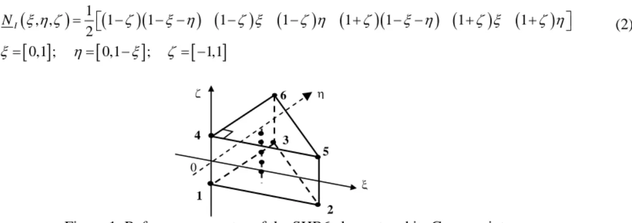
The SHB6 finite element is a solid-shell with only three displacement degrees of freedom per node, and it has a special direction called “thickness”. It is integrated with a set of five Gauss points along this direction and only one point in the in-plane directions. Figure 1 shows the SHB6 reference geometry as well as its Gauss points.
2.1 Kinematics and interpolation
The SHB6 is a linear, isoparametric element. Its spatial coordinates x and displacements i are respectively related to the nodal coordinates
i u iI
x and displacements uiI through the linear shape functions N as follows: I
and (1)
∑
= = = 6 1 ) , , ( ) , , ( I I iI I iI i x N x N x ξ ηζ ξ η ζ∑
= = = 6 1 ) , , ( ) , , ( I I iI I iI i u N u N u ξ ηζ ξ η ζHereafter, unless specified otherwise, the implied summation convention for repeated indices will be adopted. Lowercase indices vary from one to three and represent spatial coordinate directions. Uppercase indices vary from one to six and correspond to element nodes. The tri-linear isoparametric shape functions
i I I N are:
(
)
(
)(
) (
) (
) (
)(
) (
) (
)
[ ]
[
]
[
]
1 , , 1 1 1 1 1 1 1 1 2 0,1 ; 0,1 ; 1,1 I N ξ η ζ ζ ξ η ζ ξ ζ η ζ ξ η ζ ξ ζ η ξ η ξ ζ = ⎡⎣ − − − − − + − − + + ⎤⎦ = = − = − (2)Figure 1: Reference geometry of the SHB6 element and its Gauss points
0 2 1 5 3 6 4 η ζ ξ
2.2 Discrete gradient operator
Using some mathematical derivations, similarly to the procedure of the SHB8PS development reported in [1], we can explicitly express the relationship between the strain field and the nodal displacements as:
( )
, , , , , , , , , , , , , , , , , , 0 0 0 0 0 0 0 0 0 T T x x x x T T y y y y T T x z z z z s T T T T x y y x y y x x T T T T x z z x z z x x y z z y T T T T z z y y b h u b h u d b h u u d u u b h b h u u b h b h u u b h b h α α α α α α α α α α α α α α α α α α γ γ γ γ γ γ γ γ γ + + + ∇ = = ⋅ + + + + + + + + + ⎡ ⎤ ⎢ ⎥ ⎡ ⎤ ⎢ ⎥ ⎢ ⎥ ⎢ ⎥ ⎢ ⎥ ⎢ ⎥ ⎢ ⎥ ⎢ ⎥ ⎢ ⎥ ⎢ ⎥ ⎢ ⎥ ⎢ ⎥ ⎢ ⎥ ⎢ ⎥ ⎢ ⎥ ⎢ ⎥ ⎢ ⎥ ⎣ ⎦ ⎢ ⎥ ⎣ ⎦ y z B d d = ⋅ ⎡ ⎤ ⎢ ⎥ ⎢ ⎥ ⎢ ⎥ ⎣ ⎦ (3)where the hα functions are: h1=ηζ, h2 =ξζ ; the b vectors are: i bTi =N,i(0)= ∂N ∂xiξ η ζ= = =0; 1, 2, 3i= and the constant vectors γα are given by:
(
)
3 1 1, 2 1 ; 2 T i i i hα hα x b α α γ = = =
⎛
⎜
− ⋅⎞
⎟
⎝
∑
⎠
. In this latter expression,(
)
1 0, 0, 1, 0, 0, 1 ;
T
h = − hT2 =
(
0, −1, 0, 0, 1, 0)
and the x vectors denote the nodal icoordinates. We can also demonstrate the following orthogonality conditions:
0 T j x α γ ⋅ = , T hβ αβ α γ ⋅ =δ (4) 2.3 Variational principle
( )
, e T T ext V u dV d δπ ε =∫
δ ε ⋅σ −δ ⋅ f =0 (5)Replacing the assumed strain field, with its expression ε
( )
x t, = B x( ) ( )
⋅d t , in equation (5) leads to the following expression for the internal forces:( )
int e T V f =∫
B ⋅σ ε dV (6)This also leads to the following expression for the element elastic stiffness matrix:
e
T
e V
K =
∫
B ⋅ ⋅C B dV (7)Note that for a standard displacement approach, B is simply replaced with B leading to the classical stiffness:
e
T
e V
K =
∫
B ⋅ ⋅C B dV (8)2.3 Hourglass mode analysis for the SHB6 element
Hourglass modes are spurious zero-energy modes that are generated by the reduced integration. In static problems, they may lead to singularity of the assembled stiffness matrix for certain boundary conditions; in most cases this results in spurious mechanisms also known as rank deficiencies. Therefore, the analysis of hourglass modes is equivalent to that of the stiffness matrix kernel, namely zero-strain modes d that satisfy:
( )
Gj 0 GjB ζ ⋅ =d ∀ζ (9)
To this end, we can build a basis for the discretized displacements by demonstrating that the eighteen column vectors below are linearly independent. Making use of orthogonality conditions (4), we show that only the first six column vectors verify equation (9) and correspond to rigid body modes. This means that there are no hourglass modes for the SHB6 element. In other words, the SHB6 element does not require hourglass control.
⎥ ⎥ ⎥ ⎦ ⎤ ⎢ ⎢ ⎢ ⎣ ⎡ − − − 2 1 2 1 2 1 0 0 0 0 0 0 0 0 0 0 0 0 0 0 0 0 0 0 0 0 0 0 0 0 0 0 0 0 0 0 h h y x z y x S h h z x y z x S h h z y x z y S (10)
2.4 Assumed strain formulation for the SHB6 discrete gradient operator
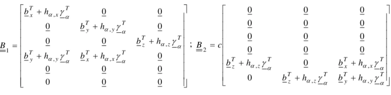
Among several treatments for alleviating shear and membrane locking, the discrete gradient is appropriately modified. This consists first of decomposing the matrix B into two parts:
2
1 B
B
B= + , then of projecting the second part onto an assumed strain operator such that
1
B =B +B
2. As a result, the stiffness matrix becomes:
1 1 1 2 2 1 2 2 1 2 3 e e e e T T T T e V V V V e e e K =
∫
B ⋅ ⋅C B dV+∫
B ⋅ ⋅C B dV+∫
B ⋅ ⋅C B dV+∫
B ⋅ ⋅C B dV=K +K +K +K 4 e (11)The subsequent steps consist of choosing an adequate assumed strain field. This is a key point in the formulation and special care has been exercised in this regard. Finally, the above additive decomposition of the stiffness matrix is calculated using a reduced integration scheme with five Gauss points. Note that the choice of an assumed strain field is mainly guided by the elimination of strain components that are responsible for shear as well as membrane locking. The advantages of this enhanced strain will be shown through benchmark problems.
⎥ ⎥ ⎥ ⎥ ⎥ ⎥ ⎥ ⎥ ⎥ ⎦ ⎤ ⎢ ⎢ ⎢ ⎢ ⎢ ⎢ ⎢ ⎢ ⎢ ⎣ ⎡ + + + + + = 0 0 0 0 0 0 0 0 0 0 0 0 0 , , , , , 1 T x T x T y T y T z T z T y T y T x T x h b h b h b h b h b B α α α α α α α α α α γ γ γ γ γ ; ⎥ ⎥ ⎥ ⎥ ⎥ ⎥ ⎥ ⎥ ⎦ ⎤ ⎢ ⎢ ⎢ ⎢ ⎢ ⎢ ⎢ ⎢ ⎣ ⎡ + + + + = T y T y T z T z T x T x T z T z h b h b h b h b c B α α α α α α α α γ γ γ γ , , , , 2 0 0 0 0 0 0 0 0 0 0 0 0 0 0
3. Numerical results and comparison
Several popular benchmark problems were performed to illustrate the element performance; one of these test problems is given here.Thisexampleisfrequentlyusedinthe literature to test warping effects on shell elements.
Figure 2: Twisted beam. Length =12; width = 1.1; depth = 0.32, twist = 90° (root to tip); E = 29x106; ν = 0.22. Loading: unit force at tip. The reference vertical displacement of point A at tip is 5.424x10⁻³
Number of elements SHB6 initial PRI6 (3D solid element) SHB6 with modification
96 0,470 0,202 0,784
192 0,779 0,485 0,935
384 0,810 0,612 0,968
Table 1: Normalized vertical displacement at point A of the twisted cantilever beam problem
4. Conclusions
This newly developed SHB6 element was implemented into the finite element codes INCA and ASTER. It represents some improvement since it converges relatively well and it performs better than the PRI6 six-node three-dimensional element in all of the benchmark problems tested. Furthermore, it shows very good performances in problems using mixed meshes composed of SHB6 and SHB8PS elements. Thus, we can couple the SHB6 with other finite elements to mesh complex geometries. For the remaining locking modes, exhibited in some test problems, a detailed study revealed that the transverse shear was behind these locking phenomena.
References
[1] Abed-Meraim F and Combescure A. SHB8PS a new adaptive, assumed-strain continuum mechanics shell element for impact analysis. Computers & Structures 2002; 80:791-803.
[2] Belytschko T and Bindeman LP. Assumed strain stabilization of the eight node hexahedral element.
Computer Methods in Applied Mechanics and Engineering 1993; 105:225-260.
[3] Hauptmann R and Schweizerhof K. A systematic development of solid-shell element formulations for linear and non-linear analyses employing only displacement degrees of freedom. International Journal for
Numerical Methods and Engineering 1998; 42:49-69.
[4] Legay A and Combescure A. Elastoplastic stability analysis of shells using the physically stabilized finite element SHB8PS. International Journal for Numerical Methods and Engineering 2003; 57:1299-1322.