Statistical analyses of the adequacy of the surface water quality monitoring network in Saskatchewan.

i

Statistical analyses of the adequacy of the

surface water quality monitoring network in

Saskatchewan

Statistical Hydrology Research Group INRS-ETE

Research Report R1276 2011

ii

Statistical analyses of the adequacy of the surface water quality monitoring

network in Saskatchewan

By

Bahaa Khalil

Chunping Ou

Sandra Proulx-McInnis

André St-Hilaire

Statistical Hydrology Research Group

Institut national de la recherche scientifique

Centre Eau, Terre et Environnement (INRS-ETE)

490 de la Couronne, Québec (Québec) G1K 9A9

Research Report R1276

iii

Reference to be cited :

Khalil, B. C. Ou, S. Proulx-McInnis, A. St-Hilaire. 2011. Statistical analyses of the adequacy of the surface water quality network in Saskatchewan. INRS-ETE Research report # R1276 prepared for the Saskatchewan Department of the Environment. . vii + 333 pages.

v

TABLE OF CONTENT

2.1  WATER QUALITY DATA ... 5 

2.2  STATISTICAL ANALYSES ... 8 

2.2.1  Preliminary analyses ... 8 

2.2.2  Statistical methods for the assessment of sampling locations ... 8 

2.2.3  Water quality variables rationalization ... 11 

2.2.4  Statistical method to estimate the appropriate sampling frequency ... 14 

3  RESULTS ... 15 

3.1  PRELIMINARY ANALYSES ... 15 

3.2  STATION LOCATIONS ... 24 

3.2.1  Principal Component Analysis ... 24 

3.2.2  Cluster Analysis ... 31 

3.3  WATER QUALITY VARIABLES ... 35 

3.4  SAMPLING FREQUENCY ... 43 

4  DISCUSSION AND CONCLUSIONS ... 52 

5  REFERENCES ... 54 

APPENDIX A: PRELIMINARY ANALYSES (KHALIL ET AL., 2011). ... 56 

APPENDIX B: ASSESSMENT AND RATIONALIZATION OF SAMPLING SITES... 59 

APPENDIX C: WATER QUALITY VARIABLES RATIONALIZATION (KHALIL ET AL., 2010B) ... 61 

APPENDIX D: CONFIDENCE INTERVAL APPROACH (KHALIL ET AL., 2011). ... 66 

APPENDIX E: PRELIMINARY ANALYSES RESULTS. ... 68 

APPENDIX G: WATER QUALITY VARIABLES RATIONALIZATION RESULTS. ... 187 

APPENDIX H: SAMPLING FREQUENCY ASSESSMENT RESULTS ... 292 

vi

LIST OF TABLES

TABLE 1.WATER QUALITY VARIABLES (WQV) SELECTED FOR THE ASSESSMENT AND REDISTRIBUTION OF

SAMPLING SITES ... 8 

TABLE 2:DESCRIPTIVE STATISTICS OF STATION SK05HG0283. ... 16 

TABLE 3:KOLGOMOROV-SMIRNOV TEST FOR STATION SK05HG0283. ... 18 

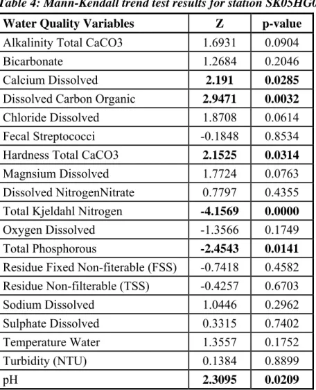
TABLE 4:MANN-KENDALL TREND TEST RESULTS FOR STATION SK05HG0283. ... 19 

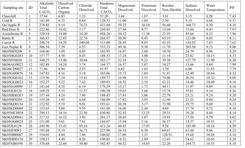
TABLE 5:MEAN VALUES OF 10 WATER QUALITY VARIABLES USED IN THE PRINCIPAL COMPONENT ANALYSIS ... 26 

TABLE 6.COMBINATIONS OF SITES TO DISCONTINUE ... 34 

TABLE 7.VARIABLE TO DISCONTINUE AND ITS BEST AUXILIARY VARIABLE ... 37 

TABLE 8.COMBINATIONS OF TWO VARIABLES TO DISCONTINUE ... 38 

TABLE 9.COMBINATIONS OF THREE VARIABLES TO DISCONTINUE ... 38 

TABLE 10.COMBINATIONS OF FOUR VARIABLES TO DISCONTINUE ... 39 

TABLE 11.COMBINATIONS OF FIVE VARIABLES TO DISCONTINUE ... 39 

TABLE 12.PAIRS OF LOCATIONS CONSIDERED FOR WATER QUALITY VARIABLES COMPARISON ... 40 

TABLE 13.WATER QUALITY VARIABLES PROPOSED TO BE MEASURED AT MOE SITES ... 42 

vii

LIST OF FIGURES

FIGURE 1.MAP SHOWING SAMPLING SITES ... 6 

FIGURE 2.FLOW CHART OF THE PROPOSED RATIONALIZATION APPROACH (MODIFIED BASED ON KHALIL ET AL, 2010A FIGURE 2) ... 13 

FIGURE 3.CORRELOGRAMS FOR THE WATER QUALITY VAIRIABLE MEASUREMENTS AT STATION SK05HG0283. ... 20 

FIGURE 4.VARIANCE EXPLAINED BY EACH PRINCIPAL COMPONENT. ... 27 

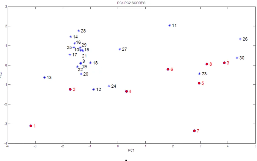
FIGURE 5.STATION SCORES IN PC1-PC2 SPACE.RED DOTS INDICATE ENVIRONMENT CANADA STATIONS... 28 

FIGURE 6.STATION SCORES IN PC1-PC3 SPACE.RED DOTS INDICATE ENVIRONMENT CANADA STATIONS... 29 

FIGURE 8.DENDOGRAM SHOWING CLUSTER ANALYSIS RESULTS. ... 32 

FIGURE 9.CLUSTER TREE FOR WATER QUALITY VARIABLES AT SK05HG0283 ... 36 

FIGURE 10.NUMBER OF SAMPLES VS. EXPECTED ERROR FOR THE DISSOLVED CHLORIDE MEASURED AT SAMPLING SITE SK05HG0283. ... 44 

FIGURE 11.NUMBER OF SAMPLES VS. EXPECTED ERROR FOR DISSOLVED ORGANIC CARBON MEASURED AT SAMPLING SITE SK05HG0283. ... 45 

FIGURE 12.NUMBER OF SAMPLES VS. EXPECTED ERROR FOR FECAL STREPTOCOCCI MEASURED AT SAMPLING SITE SK05HG0283. ... 45 

FIGURE 13.NUMBER OF SAMPLES VS. EXPECTED ERROR FOR DISSOLVED NITRATE MEASURED AT SAMPLING SITE SK05HG0283. ... 46 

FIGURE 14.NUMBER OF SAMPLES VS. EXPECTED ERROR FOR TOTAL KJELDAHL NITROGEN MEASURED AT SAMPLING SITE SK05HG0283. ... 46 

FIGURE 15.NUMBER OF SAMPLES VS. EXPECTED ERROR FOR DISSOLVED OXYGEN MEASURED AT SAMPLING SITE SK05HG0283. ... 47 

FIGURE 16.NUMBER OF SAMPLES VS. EXPECTED ERROR FOR TOTAL PHOSPHORUS MEASURED AT SAMPLING SITE SK05HG0283. ... 47 

FIGURE 17.NUMBER OF SAMPLES VS. EXPECTED ERROR FOR FIXED NON-FILTERABLE RESIDUE MEASURED AT SAMPLING SITE SK05HG0283. ... 48 

FIGURE 18.NUMBER OF SAMPLES VS. EXPECTED ERROR FOR NON-FILTERABLE RESIDUE MEASURED AT SAMPLING SITE SK05HG0283. ... 48 

FIGURE 19.NUMBER OF SAMPLES VS. EXPECTED ERROR FOR WATER TEMPERATURE MEASURED AT SAMPLING SITE SK05HG0283. ... 49 

FIGURE 20.NUMBER OF SAMPLES VS. EXPECTED ERROR FOR TURBIDITY MEASURED AT SAMPLING SITE SK05HG0283. ... 49 

1

EXECUTIVE SUMMARY

Objectives

The main goal of this study is to assess the adequacy of the Saskatchewan surface water quality monitoring network. To achieve this goal, three specific objectives are defined as follows:

 Assessment of the location of sampling sites;

 Assessment and reselection of water quality variables to be measured;  Assessment of sampling frequency.

Main Results

After performing a number of preliminary statistical analyses to assess the quality and distribution of the data, two multivariate approaches were used to evaluate potential similarities or redundancies between stations. To achieve this, the analysis was limited to ten water quality variables that were most frequently sampled at all stations. They are: Alkalinity, Dissolved Organic Carbon, Hardness, Dissolved magnesium, Dissolved potassium, Non-filterable Residues, Sodium, Temperature and pH.

Both multivariate methods, Principal Component Analysis (PCA) and Cluster Analysis (CA) indicate that numerous provincial stations have great similarities, while Environment Canada (EC) stations are less similar. Both PCA and CA show that the majority of EC stations have distinct water quality information. These stations are located on the Churchill, Qu’Appelle, Red Deer, Carrot and East Poplar Rivers.

In addition, Cluster analysis identified five provincial stations that seem to have unique information and that should be prioritized to remain in the network. They are: SK06AD0041, SK05JL0129, SK05JF0092, SK05HB0087 and SK05NB0198.

Both methods showed that there are a few pairs of stations with similar information. They are:

2

 Assiniboine River (SA05MD0002) and SK05MC0038  Churchill River (SA06EA0003) and SK06CD0027

Assessment of water quality variables was carried out for each of the MOE sampling site. The analysis was limited to water quality variables that were most frequently sampled at each sampling site. Results indicate that there are information redundancies among water quality variables and considerable number of variables could be discontinued. The maximum number of variables to be discontinued varies between five variables for sampling sites SK05HG0283 and SK05HH0267 and 14 variables at sampling site SK05JF0092. Detailed results for each sampling site are presented in Appendix G.

Water quality variables assessment was carried out for the EC sampling sites to identify variables that are measured by the EC network and may be added to the list of variables measured at MOE sites. This analysis was carried out for four pairs of EC and MOE sites that are considered similar and are located on the same watershed. Results showed that few variables may be added to the list of variables measured at two MOE sampling sites. Specifically, Lithium and Delta-Benzenehexachloride could be added to list of variables measured at Battle River (SK05FF0020). The 1,2,4,5-Tetrabromobenzene, 2,3-D, Clopyralid, Delta-Benzenehexachloride, Endrin, Gamma-Benzenehexachloride and Lithium could be added to the list of variables measured at Assiniboine (SK05MC0038). However, final decision for adding these variables should be taken after reviewing watershed attributes.

Sampling frequency was analyzed using a statistical estimation based on the confidence interval around the mean value of each water quality variable. Identification of the required number of samples to estimate the mean with minimum error varies between water quality variables and from site to site. Based on analyses carried out for each sampling site, the water quality variables may be divided into four groups. The first group of variables could be sampled four times per year to estimate the mean value with a relatively small margin of error. Water quality variables of the second and third groups would require respectively 6 and 12 samples per year to achieve a similarly acceptable level of error. Given the large variability, variables of the fourth group would require higher sampling frequency, perhaps as high as biweekly in order to get an estimate of the mean value with acceptable uncertainty. Detailed results for each water quality variable at each of the MOE sampling sites are presented in Appendix H. In general the following water quality variables require six samples per year, while other variables require larger number of samples:

3  Alkalinity Total CaCO3

 Barium  Bicarbonate  Beryllium  Boron  Calcium Dissolved  Calcium Total

 Carbon Dissolved inorganic  Carbon Total inorganic  Carbon Total

 Fluoride Dissolved  Hardness Total CaCO3  Specific Conductance  Sulphate

 Total Dissolved Solids  pH

4

1 INTRODUCTION

1.1 Context

Surface water quality monitoring is one of the responsibilities of a number of provincial and federal environmental departments in Canada.

In Saskatchewan, the Ministry of Environment (MOE) is responsible for 23 surface water quality monitoring stations. The sampling effort was initiated 40 years ago, and has been ongoing since with varying degrees of spatial and temporal coverage.

In recent years, one of the main uses of these water quality data is the calculation of a Water Quality Index (WQI, Lumb et al., 2006). The WQI is an attempt to summarize water quality data in order to provide managers and policy makers with the necessary information for decision-making. The WQI is based in part on the comparison of measurements with known standards or guidelines. The number of variables not meeting these standards, the frequency of exceedance and the amplitude of the exceedances are accounted for. A suite of water quality variables are therefore measured and compiled by MOE to perform these calculations. The adequacy of the sampling network to perform this task needs to be validated.

In addition to the 23 provincial water quality stations, Environment Canada (EC) monitors water quality at a number of sites in Saskatchewan. However, some of the EC stations are in close proximity to MOE monitoring stations. It is therefore possible that some redundancy exists in the joint EC-MOE network.

1.2 Objectives

The main goal of the present study is to provide a first statistical assessment of the surface water quality monitoring network in Saskatchewan. The specific objectives of the study include:

 Assessment of sampling frequency;

 Assessment of the location of sampling sites;

5

2 METHODS

2.1 Water Quality Data

Two water quality datasets were used in this study. The first dataset was provided by the Environmental Protection and Audit division of the Ministry of Environment of Saskatchewan. The dataset consists of 23 sampling sites, through which the number of variables measured ranges from 36 to 51, with an irregular sampling frequency. Measurements span the period of January 1975 to February 2011.

The second dataset was provided by Environment Canada. The dataset consists of nine sampling sites, where more than 200 water quality variables are measured on irregular frequency since September 1966 to June 2010. Figure 1 shows the locations of both provincial and federal stations.

Both datasets exhibit large gaps and large number of censored data. Several preparation steps were carried out before data analyses took place.

The first preparation step was to remove censored data. These data include measurements labelled as ‘less than’ or ‘below detection limit’. Below detection data arise as a result of the technological limits of laboratory instrumentation (Zhu and McBean, 2004). Since the actual value remains uncertain, the censored data were removed.

The second preparation step was to rearrange data on a monthly basis, to identify the gaps. In some cases there were two samples taken during the same day or month, which were analyzed for different water quality variables, and considered as complementary samples. In this case, the two samples were combined to have one set of water quality observations for this month.

6

Figure 1. Map showing sampling sites

t

D

o

~\L

COOOI

7 The third preparation step was to screen both datasets to identify water quality variables that have 30 or more valid records during the monitoring period from September 1966 to February 2011. Water quality variables that have less than 30 records were excluded from further analysis. Two sites were thus excluded:

 Sampling site US05ND0004 at the Souris River near Sherwood, where only twelve samples were collected from September 1999 to August 2010 (The maximum number of observations available is 12); and

 Sampling site SK05JF0595 at the Qu’Appelle River (SA05JM0014), where sampling started on May 2006 and ended on November 2007 (The maximum number of available observations is 9).

In the fourth step, a logical check was performed to identify potential outliers or faulty data to be removed. For example:

 Fecal Coliform was 60 no/100 ml while Total Coliform was only 20 no/100 ml (Sample 2005003713, 14/9/2005 at Station SK06AD0041);

 Dissolved Silver was 0.011 µg/l while Total Silver was 0.007 µg/l (Sample 2004PN090017, 12/5/2004 at Station SA05FE001, Battle River);

 Dissolved Selenium was 0.29 µg/l and 0.13 µg/l while Total Selenium was 0.28 µg/l and 0.09 µg/l for samples 2003PN090054 and 2003PN090100 respectively. These samples were taken on 22/7/2003 and 5/11/2003, respectively, at Station SA05FE001, Battle River;

 Dissolved Antimony was 0.114 µg/l while Total Antimony was 0.112 µg/l (Sample 2009PN290242, 20/1/2010 at Station SA05KH0002, Carrot River).

In the fifth step, any variable that has more than 30 valid records were included in the assessment of sampling frequency. For the assessment and redistribution of monitoring locations, variables that have more than 30 records and being measured at all 22 MOE sampling sites and nine Environment Canada sites were included. Only ten water quality variables were selected based on these criteria. They are shown in Table 1.

8

Table 1. Water quality variables (WQV) selected for the assessment and redistribution of sampling sites

WQV Alkalinity Total CaCO3 Carbon Dissolved Organic Chloride Dissolved Hardness Total CaCO3 Magnesium Dissolved Units mg/l mg/l mg/l mg/l mg/l WQV Potassium Dissolved Residue Non-filterable (TSS) Sodium Dissolved Temperature pH

Units mg/l mg/l mg/l deg C pH units

2.2 Statistical Analyses

The first step in the methodology is to carry out preliminary analyses in order to understand the water quality data characteristics and to check the statistical assumptions required to apply the designed statistical approaches. Statistical methods are then applied to assess the sampling frequency (section 2.2.1) and sampling locations (section 2.2.2).

2.2.1 Preliminary analyses

The preliminary analyses applied in this study include: calculation of descriptive statistics, tests to check normality in the distribution of each water quality variable, existence of trend and autocorrelation. The descriptive statistics include measures of central tendency (mean, median), dispersion (variance, standard deviation, maximum and minimum) and the shape of the distribution (skewness, kurtosis). Kolomogrov-Smirnov goodness of fit test was applied to check normality. Modified Mann-Kendall autocorrelation test was applied for trend detection. The detailed method for each test is provided in Appendix A.

2.2.2 Statistical methods for the assessment of sampling locations

The proposed approach for the assessment and rationalization of sampling sites is based on two multivariate statistical techniques. These techniques are the principal component analysis (PCA) and cluster analysis (CA).

9 PCA calculates linear combinations of the original water quality variables. These linear combinations must satisfy different criteria: 1) the linear combinations must explain the maximum possible variability in the original data set; and 2) the sum of the weights of the linear combination must equal 1. The first principle component (PC1) is therefore the linear combination of the original variables that explains the largest proportion of the sample variance. The second principal component (PC2) will be a linear combination of original variables that maximizes explained residual variance (i.e. variance left once PC1 is removed) and so on. Typically, the first few (e.g. 3) PCs will explain the majority of the sample variance. It is then possible to calculate the coordinates of each station associated with PC1, PC2, PC3, etc. These coordinates, called scores, can be plotted in PC space (a Cartesian coordinate system in which PC1 is the X coordinate and PC2 or PC3 is the Y coordinate). Stations that are close together in PC space are similar. Potential redundant stations can thus be identified.

CA is an exploratory data technique used to group similar observations into clusters, where the within-cluster variance is minimized and the between-within-cluster variance is maximized (Jobson, 1992). An agglomerative hierarchical cluster algorithm was employed to identify clusters of similar sampling sites based on their principle component scores.

The main objective from the proposed approach is to identify similar sampling sites and possible sites to be discontinued. This approach consists of four main steps. In the first step, PCA is employed to convert original water quality variables into new uncorrelated variables (principle components) for each of the monitoring sites. In the second step, monitoring sites are projected in PC space to identify similar stations. The third step is to verify the conclusions of PCA using CA. The forth step is to identify the optimal combination of sites to discontinue using an information index.

Assume that the variable y measured at a discontinued monitoring location Y has n₁ years of data and

that the variable x measured at a continuously monitored location X has n₁  years of which n₂ n₁ are

concomitant with the data observed at Y, illustrated as follows:

1 2 1 1 1 1

,...,

,

,

:

)

(

,...,

,

,

,...,

,

,

:

)

(

y

y

y

y

Y

Location

x

x

x

x

x

x

x

X

Location

10

Consider that year n₁ is the year when the assessment and redesign took place. After n₁ years, a decision

is made to stop monitoring at location Y and continue measuring at location X. Assume that after n₂

years, our interest is to reconstitute information about water quality variables at discontinued locations. Matalas and Jacobs (1964) developed a procedure for obtaining unbiased estimators of the mean ( ) _y and the variance ( 2

y

 ), showing that the mean value (ˆ_y) of the extended Y series can be determined using the following equation:

)

(

ˆ

ˆ

x

x

n

n

n

y





_







where y₁ and x₁ are the mean values of y and _i x , respectively, based on the short records _i i1,...,n₁,

2

x is the mean value of x observed during the period _i in₁1,....,n₂ and the parameter ˆ is the estimated regression coefficient. Based on this formulation, it is possible to show (Cochran, 1953) that the variance of ˆy is given by:

 

 is the population variance of y and



(Ouarda et al, 1996).

To define the optimal combination of sampling sites to be continuously measured and those to be discontinued, consider the case where k sampling sites to be discontinued. Which k sites among the available 23 MOE sites should be selected? The number of possible combinations of sites to discontinue is given by the binomial coefficient C(23,k). For each combination, an information index is employed according to which the combinations may be ranked. Such a procedure allows the identification of the best combination of sampling sites to discontinue, or provides the decision maker with the rank of the best combinations to discontinue. An aggregated information index (Ia) is defined as follows:

11

 









where X is the water quality variable and Var



 



For the discontinued sites, the variance of the mean value estimator after n2 years is estimated using

Equation 2. For continuously measured variables, the variance of the mean value after n2 years is assumed

to be equal to the variance of the mean after n1 years multiplied by (n1-1)/( n1+ n2-1) (Khalil et al.,

2010a). The proposed approach details are presented in Appendix B.

2.2.3 Water quality variables rationalization

The Correlation-Regression (CR) approach is the most commonly used statistical approach to reduce the number of water quality variables being measured. As described by Khalil and Ouarda (2009) the CR approach is based on three steps: First, correlation analysis is used to assess the level of association among the variables being measured. If high correlation exists among the variables, some of the information produced may be redundant. Second, the water quality variables to be continuously measured or discontinued are selected. This step is based on some subjective criteria, such as the significance of the variable, the presence of the variable in local or international standards. It may be based also on the cost of laboratory analysis. Third, the reconstitution of information about the discontinued variables using auxiliary variables from the continuously measured variables is examined.

Khalil et al. (2010a) modified the CR approach to overcome two main deficiencies. The first deficiency involves the method used to identify highly associated variables. The correlation coefficient is commonly used as a criterion to assess the level of association, but selection of the proper threshold above which a correlation coefficient can be considered sufficient to associate two variables can be problematic. Assessment of the correlation coefficient is always based on subjective preference. Thus, studies using the same variables but performed by different investigators may lead to different results. The second deficiency is the absence of a criterion to identify the combination of variables that should be continuously measured or discontinued. In the modified CR, Khalil et al. (2010) used criteria from record-augmentation procedures to identify a correlation coefficient threshold; and an information index to identify optimal combinations of variables to be continuously measured and variables to discontinue.

12

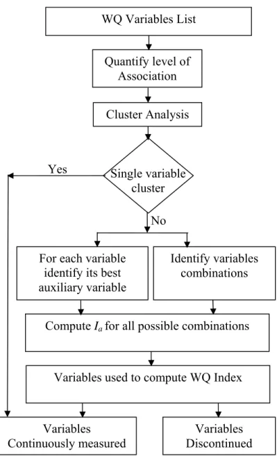
The approach proposed by Khalil et al. (2010a) consists of three main steps. The first step involves correlation analysis, cluster analysis and correlation coefficient threshold to assess the level of association among the variables being measured and to define the groups of variables that are highly associated. Then, for each highly associated group of variables, the second step is to assume that each variable within the group would be discontinued and to identify the best auxiliary variable from the same group. The third step is to assess different combinations of variables to be discontinued and variables to be continuously measured using an information index. In this study, the approach proposed by Khalil et al. (2010a) was applied to identify optimal combinations of variables to be continuously measured and variables to discontinue for the Saskatchewan water quality monitoring network. Figure 2 illustrates the flow of the analyses. Detailed analyses are described in Appendix C.

The same approach was applied for Environment Canada water quality monitoring network. The objective was to identify if some of the extra variables that are measured through the EC monitoring network should be measured by the MOE network. The extra EC variables were assessed relative to other variables within each of the EC sampling sites separately. If the extra variable is highly correlated with one of the MOE variables, it indicates that there is information redundancy and therefore there is no need to add this variable to the MOE network. If the extra variable is not highly correlated with one of the MOE variables, it indicates that this variable may be added to the list of variables measured by the MOE.

13 Figure 2. Flow chart of the proposed rationalization approach (modified, based on Khalil et al, 2010a

Figure 2)

WQ Variables List

For each variable identify its best auxiliary variable

Quantify level of Association

Compute Ia for all possible combinations

Variables Continuously measured Variables Discontinued Identify variables combinations Single variable cluster Cluster Analysis No Yes

14

2.2.4 Statistical method to estimate the appropriate sampling frequency

In this study the confidence interval around the mean is used as a criterion for the assessment of the sampling frequency. This approach assumes that the monitoring objectives are the determination of ambient water quality status and an assessment of annual means.

The confidence interval approach allows selecting a sampling frequency that yields an estimate of the sample mean (x ) within a prescribed degree of accuracy (confidence limits) (Khalil et al., 2011).

A formula for sample size is based on the assumption that the water quality observations are stationary (i.e. no temporal trends). Based on the preliminary analyses, water quality variables that exhibit trend were de-trended, and then examined for autocorrelation. If autocorrelation function is not significant at lag-1, the original formula proposed by Sanders and Adrian (1978) was used.

2 2 /      E s t n  (4)

where n is the number of samples that need to be taken to estimate the mean with an error E, at a level of confidence 1-α , s is the sample standard deviation, t_/2 is the Student’s “t” statistic at an acceptable

confidence level (1-) and the error (E) is the difference between the true population mean and the sample mean (x). In this study E is considered as a percentage of the sample mean. Hence the minimum number of samples required is always given for a pre-stated error level, which is deemed acceptable by the manager. In the present analysis, different error levels were tested.

In case the autocorrelation function is significant, the modified formula provided by Loftis and Ward (1979) and simplified by Gilbert (1987) was used in this study.

       



where k is the autocorrelation coefficient for lag k , 2

s _{is the sample variance, A detailed mathematical} explanation is provided in Appendix D.

15

3 RESULTS

3.1 Preliminary analyses

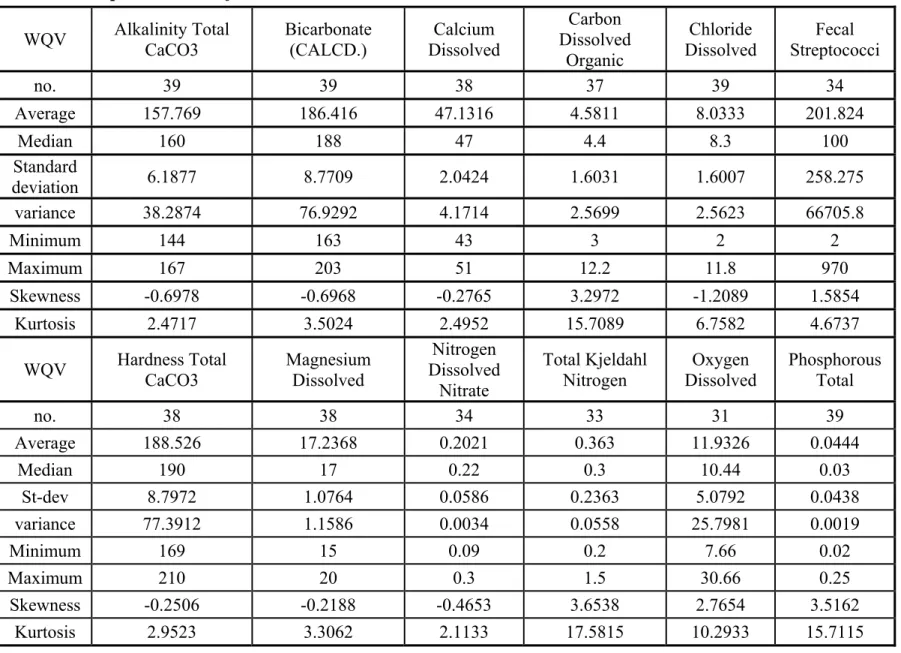
The results of the preliminary analyses for sampling site SK05HG0283 are presented here as an example of the preliminary analyses applied for each of the sampling sites under assessment. Detailed results for each sampling site are presented in Appendix E. Following data preparation and validation, 19 water quality variables were considered for further analyses at sampling site SK05HG0283. Table 2 shows the descriptive statistics for the 19 water quality variables measured at sampling site SK05HG0283. The maximum number of monthly records available ranges between 31 observations for Dissolved Oxygen to 39 observations for Total Alkalinity (CaCO3), Bicarbonate, Dissolved Chloride, Total Phosphorus, Fixed Non-filterable Residues (FSS), Non-filterable Residue (TSS) and pH.

For sampling site SK05HG0283, the average and median for most of the variables were very similar, indicating that the distributions of the measurements of each of these variables were essentially symmetric. The Fecal Streptococci shows a large difference between the average and the median, where the average is two folds the median value. The coefficient of variation is the ratio of the standard deviation to the average. The coefficient of variation indicated a low variability for 7 of the 19 variables considered at this sampling site. Low coefficients of variation range between 2.1% for pH to 11% for Sodium. Three variables show high coefficient of variation, 86% for Water Temperature, 98% for Total Phosphorous and 128% for Fecal Streptococci.

The skewness and kurtosis values for most of the variables indicated that the observations were symmetric around their mean value, with normal tails. Large tails and strong positive skewness were detected for the Dissolved organic Carbon, Fecal streptococci, Total Kjeldahl Nitrogen, Oxygen Dissolved and Total Phosphorous while negative skewness was detected for pH.

16 Table 2: Descriptive statistics of station SK05HG0283.

WQV Alkalinity Total _CaCO3 Bicarbonate _{(CALCD.) Dissolved} Calcium

Carbon Dissolved Organic Chloride Dissolved Fecal Streptococci no. 39 39 38 37 39 34 Average 157.769 186.416 47.1316 4.5811 8.0333 201.824 Median 160 188 47 4.4 8.3 100 Standard deviation 6.1877 8.7709 2.0424 1.6031 1.6007 258.275 variance 38.2874 76.9292 4.1714 2.5699 2.5623 66705.8 Minimum 144 163 43 3 2 2 Maximum 167 203 51 12.2 11.8 970 Skewness -0.6978 -0.6968 -0.2765 3.2972 -1.2089 1.5854 Kurtosis 2.4717 3.5024 2.4952 15.7089 6.7582 4.6737

WQV Hardness Total _CaCO3 Magnesium _Dissolved

Nitrogen Dissolved Nitrate Total Kjeldahl Nitrogen Oxygen Dissolved Phosphorous Total no. 38 38 34 33 31 39 Average 188.526 17.2368 0.2021 0.363 11.9326 0.0444 Median 190 17 0.22 0.3 10.44 0.03 St-dev 8.7972 1.0764 0.0586 0.2363 5.0792 0.0438 variance 77.3912 1.1586 0.0034 0.0558 25.7981 0.0019 Minimum 169 15 0.09 0.2 7.66 0.02 Maximum 210 20 0.3 1.5 30.66 0.25 Skewness -0.2506 -0.2188 -0.4653 3.6538 2.7654 3.5162 Kurtosis 2.9523 3.3062 2.1133 17.5815 10.2933 15.7115

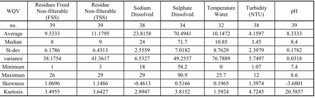
17 Table 2: Descriptive statistics of station SK05HG0283(continued).

WQV Residues Fixed Non-filterable (FSS) Residue Non-filterable (TSS) Sodium

Dissolved Dissolved Sulphate Temperature Water Turbidity (NTU) pH

no. 39 39 38 34 32 38 39 Average 9.3333 11.1795 23.8158 70.4941 10.1472 4.1597 8.3333 Median 8 9 24 71.7 10.85 3.45 8.4 St-dev 6.1786 6.4313 2.5559 7.0182 8.7629 2.3979 0.1782 variance 38.1754 41.3617 6.5327 49.2557 76.7889 5.7497 0.0318 Minimum 1 3 18 58.2 0 1.07 7.4 Maximum 26 29 29 90.9 25.7 12 8.6 Skewness 1.0696 1.1486 -0.4613 0.5166 0.1965 1.3974 -3.6801 Kurtosis 3.4955 3.6427 2.8947 3.8152 1.5924 4.7245 20.5857

18

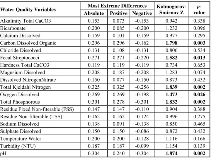
To check normality, the Kolmogorov-Smirnov goodness of fit test was used (Table 3). The test results indicated that the null hypothesis (data are normally distributed) cannot be rejected at a 5% level of significance (p-value is the probability of accepting the null-hypothesis) for most of the variables (Table 3), whereas for 6 variables, the null hypothesis cannot be accepted. For the variables that do not follow the normal distribution, Box-Cox transformation was applied to achieve normality.

Table 3: Kolgomorov-Smirnov test for station SK05HG0283.

Water Quality Variables Most Extreme Differences

Kolmogorov-Smirnov Z

p-value

Absolute Positive Negative

Alkalinity Total CaCO3 0.153 0.073 -0.153 0.942 0.338

Bicarbonate 0.200 0.085 -0.200 1.232 0.096 Calcium Dissolved 0.159 0.101 -0.159 0.977 0.295

Carbon Dissolved Organic 0.296 0.296 -0.162 1.798 0.003

Chloride Dissolved 0.131 0.108 -0.131 0.806 0.534 Fecal Streptococci 0.271 0.271 -0.220 1.582 0.013

Hardness Total CaCO3 0.119 0.119 -0.119 0.734 0.653 Magnsium Dissolved 0.208 0.187 -0.208 1.283 0.074 Dissolved NitrogenNitrate 0.150 0.077 -0.150 0.873 0.432 Total Kjeldahl Nitrogen 0.325 0.325 -0.256 1.839 0.002

Oxygen Dissolved 0.269 0.269 -0.198 1.473 0.026

Total Phosphorous 0.301 0.278 -0.301 1.832 0.002

Residue Fixed Non-fiterable (FSS) 0.147 0.147 -0.110 0.904 0.388 Residue Non-filterable (TSS) 0.162 0.162 -0.124 0.996 0.275 Sodium Dissolved 0.138 0.091 -0.138 0.850 0.465 Sulphate Dissolved 0.150 0.150 -0.086 0.872 0.432 Temperature Water 0.200 0.200 -0.128 1.116 0.166 Turbidity (NTU) 0.187 0.187 -0.099 1.154 0.139 pH 0.304 0.240 -0.304 1.874 0.002

The modified Mann-Kendall non-parametric trend test was applied. Table 4 shows the results for the variables measured at sampling site SK05HG0283. The Z statistic and the probability of accepting the null hypothesis (p-value) suggested there was no trend in most of the variables measured at this sampling site. The null hypothesis could not be rejected for any of the remaining variables at station SK05HG0283 and for 5 variables, Dissolved Carbon, Hardness Total CaCO3,

19 Total Kjeldahl Nitrogen, Total Phosphorous and pH. Water quality variable that showed a significant trend were de-trended before autocorrelation analysis as well as for the sampling frequency assessment.

Table 4: Mann-Kendall trend test results for station SK05HG0283.

Water Quality Variables Z p-value

Alkalinity Total CaCO3 1.6931 0.0904

Bicarbonate 1.2684 0.2046 Calcium Dissolved 2.191 0.0285

Dissolved Carbon Organic 2.9471 0.0032

Chloride Dissolved 1.8708 0.0614 Fecal Streptococci -0.1848 0.8534 Hardness Total CaCO3 2.1525 0.0314

Magnsium Dissolved 1.7724 0.0763 Dissolved NitrogenNitrate 0.7797 0.4355 Total Kjeldahl Nitrogen -4.1569 0.0000

Oxygen Dissolved -1.3566 0.1749 Total Phosphorous -2.4543 0.0141

Residue Fixed Non-fiterable (FSS) -0.7418 0.4582 Residue Non-filterable (TSS) -0.4257 0.6703 Sodium Dissolved 1.0446 0.2962 Sulphate Dissolved 0.3315 0.7402 Temperature Water 1.3557 0.1752 Turbidity (NTU) 0.1384 0.8899 pH 2.3095 0.0209

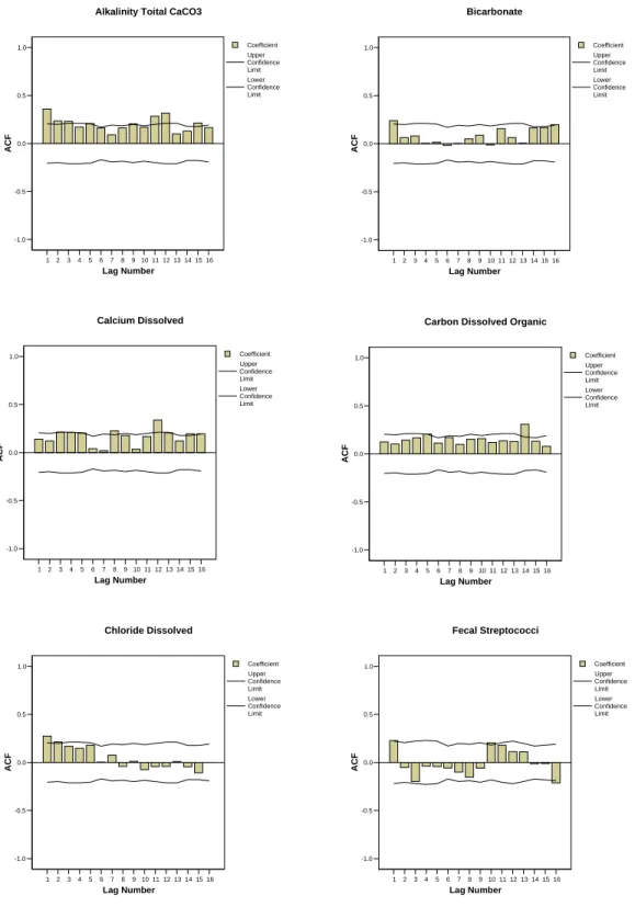
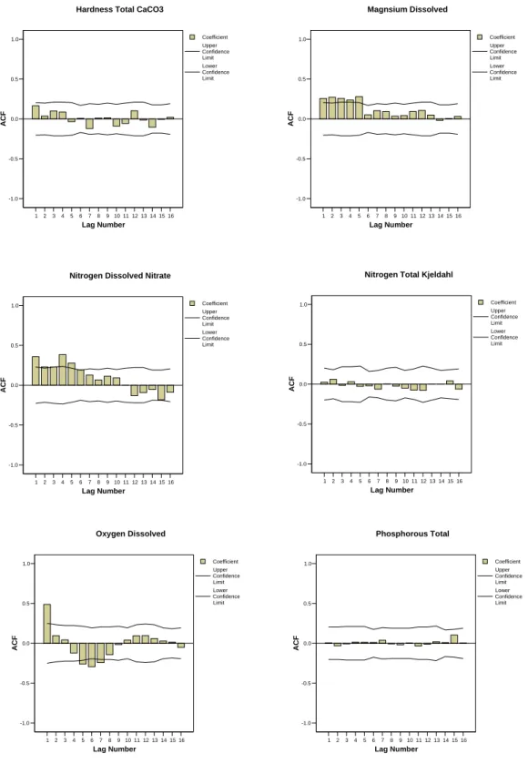
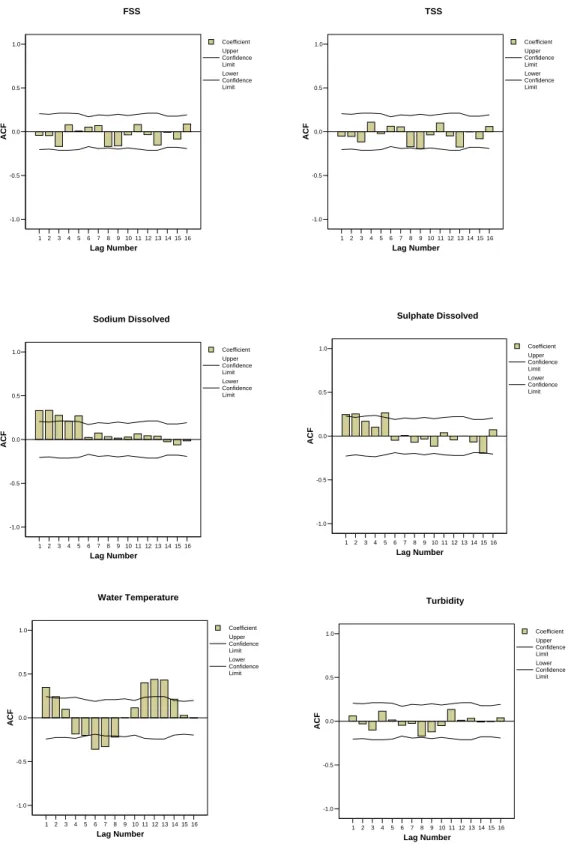
The autocorrelation functions (ACFs) were computed for the variables measured at sampling site SK05HG0283. Figure 2 shows the correlograms for the first 16 lags (monthly basis) for each of the 19 variables measured at SK05HG0283. Figure 3 shows that the autocorrelation was significant in 12 out of the 19 variables. Thus, sampling frequency assessment using the confidence interval approach was applied using the formula proposed by Sanders and Adrian (1978) for the water quality variables that showed no autocorrelation. For water quality variables that showed significant autocorrelation, the formula modified by Loftis and Ward (1979) and simplified by Gilbert (1987) was used.

20 Figure 3. Correlograms for the water quality vairiable measurements at station SK05HG0283.

1 2 3 4 5 6 7 8 9 10 11 12 13 14 15 16 Lag Number -1.0 -0.5 0.0 0.5 1.0 ACF Coefficient Upper Confidence Limit Lower Confidence Limit

Alkalinity Toital CaCO3

1 2 3 4 5 6 7 8 9 10 11 12 13 14 15 16 Lag Number -1.0 -0.5 0.0 0.5 1.0 ACF Coefficient Upper Confidence Limit Lower Confidence Limit Bicarbonate 1 2 3 4 5 6 7 8 9 10 11 12 13 14 15 16 Lag Number -1.0 -0.5 0.0 0.5 1.0 ACF Coefficient Upper Confidence Limit Lower Confidence Limit Calcium Dissolved 1 2 3 4 5 6 7 8 9 10 11 12 13 14 15 16 Lag Number -1.0 -0.5 0.0 0.5 1.0 ACF Coefficient Upper Confidence Limit Lower Confidence Limit

Carbon Dissolved Organic

1 2 3 4 5 6 7 8 9 10 11 12 13 14 15 16 Lag Number -1.0 -0.5 0.0 0.5 1.0 ACF Coefficient Upper Confidence Limit Lower Confidence Limit Fecal Streptococci 1 2 3 4 5 6 7 8 9 10 11 12 13 14 15 16 Lag Number -1.0 -0.5 0.0 0.5 1.0 ACF Coefficient Upper Confidence Limit Lower Confidence Limit Chloride Dissolved

21 Figure 3. (continued). Collerograms for the water quality variables measurements at

SK05HG0283 1 2 3 4 5 6 7 8 9 10 11 12 13 14 15 16 Lag Number -1.0 -0.5 0.0 0.5 1.0 ACF Coefficient Upper Confidence Limit Lower Confidence Limit

Hardness Total CaCO3

1 2 3 4 5 6 7 8 9 10 11 12 13 14 15 16 Lag Number -1.0 -0.5 0.0 0.5 1.0 ACF Coefficient Upper Confidence Limit Lower Confidence Limit Magnsium Dissolved 1 2 3 4 5 6 7 8 9 10 11 12 13 14 15 16 Lag Number -1.0 -0.5 0.0 0.5 1.0 ACF Coefficient Upper Confidence Limit Lower Confidence Limit

Nitrogen Dissolved Nitrate

1 2 3 4 5 6 7 8 9 10 11 12 13 14 15 16 Lag Number -1.0 -0.5 0.0 0.5 1.0 ACF Coefficient Upper Confidence Limit Lower Confidence Limit

Nitrogen Total Kjeldahl

1 2 3 4 5 6 7 8 9 10 11 12 13 14 15 16 Lag Number -1.0 -0.5 0.0 0.5 1.0 ACF Coefficient Upper Confidence Limit Lower Confidence Limit Oxygen Dissolved 1 2 3 4 5 6 7 8 9 10 11 12 13 14 15 16 Lag Number -1.0 -0.5 0.0 0.5 1.0 ACF Coefficient Upper Confidence Limit Lower Confidence Limit Phosphorous Total

22 Figure 3. (continued). Collerograms for the water quality variables measurements at

SK05HG0283 1 2 3 4 5 6 7 8 9 10 11 12 13 14 15 16 Lag Number -1.0 -0.5 0.0 0.5 1.0 ACF Coefficient Upper Confidence Limit Lower Confidence Limit FSS 1 2 3 4 5 6 7 8 9 10 11 12 13 14 15 16 Lag Number -1.0 -0.5 0.0 0.5 1.0 ACF Coefficient Upper Confidence Limit Lower Confidence Limit TSS 1 2 3 4 5 6 7 8 9 10 11 12 13 14 15 16 Lag Number -1.0 -0.5 0.0 0.5 1.0 ACF Coefficient Upper Confidence Limit Lower Confidence Limit Sodium Dissolved 1 2 3 4 5 6 7 8 9 10 11 12 13 14 15 16 Lag Number -1.0 -0.5 0.0 0.5 1.0 ACF Coefficient Upper Confidence Limit Lower Confidence Limit Sulphate Dissolved 1 2 3 4 5 6 7 8 9 10 11 12 13 14 15 16 Lag Number -1.0 -0.5 0.0 0.5 1.0 ACF Coefficient Upper Confidence Limit Lower Confidence Limit Water Temperature 1 2 3 4 5 6 7 8 9 10 11 12 13 14 15 16 Lag Number -1.0 -0.5 0.0 0.5 1.0 ACF Coefficient Upper Confidence Limit Lower Confidence Limit Turbidity

23 Figure 3. (continued). Collerograms for the water quality variables measurements at

SK05HG0283 1 2 3 4 5 6 7 8 9 10 11 12 13 14 15 16 Lag Number -1.0 -0.5 0.0 0.5 1.0 ACF Coefficient Upper Confidence Limit Lower Confidence Limit pH

24

3.2 Station locations

3.2.1 Principal Component Analysis

Principal components were calculated using the matrix of mean water quality values presented in Table 5. Figure 4 shows the variance explained by each principal component. The first three principal components explain 50%, 15% and 12 % of the variance, respectively.

Loadings are correlations between the original variables and each principal component. Total Alkalinity (CaCO3), Dissolved Organic Carbon, Total Hardness (CaCO3), Magnesium, Potassium and Sodium (Dissolved/Filtered) are the variables that contributed the most to the first PC with loadings of 0.38, 0.32, 0.42, 0.42, 0.43 and 0.39, respectively. For PC2, Water temperature and pH are the variables that contributed the most to explained variance, with values of 0.57 and 0.63, respectively. Finally, the Non-filterable Residue is the main variable defining the third PC, with a loading of 0.73.

Figures 5-7 show the station scores in PC1-PC2, PC1-PC3 and PC2-PC3 space, respectively. Most Environment Canada (EC) stations are distributed along the PC1 gradient, with PC1 scores ranging between -3 and 4 (Figure 5). There are two notable exceptions: station 1 (Churchill River, SAE6EA0003) and station 7 (Carrot River near TurnB, SAO5KH0002) have high negative (<-3) scores on PC2, an indication that the variability in water quality for these two stations is mostly determined by pH and Water Temperature.

Since PC3 explains nearly as much variance as PC2, it was also used to create Cartesian spaces with PC2 (Figure 6) and PC1 (Figure 7). Station 7 (Carrot River near Turn B) has high negative loading on PC2 and PC3, and is isolated from most stations. This is an indication that its water quality properties are quite different than most stations. In contrast, EC stations 5 and 8 are relatively close in all PC spaces.

Station 23 (SK05MC0038) is located in close proximity to EC stations 5 and 8, as shown in Figures 5 to 7 and therefore displays similarities in mean water quality (as defined by the 10 variables in Table 5) as EC stations 5 (Assiniboine River) and 8 (East Poplar River,

SA11AE0008). EC station 4 (Red Deer River, SAO5LC0001) and provincial station 24 (SK06AD0041) are also close in all PC spaces. Their score on PC1 is near zero, while it is approximately -1 on PC2 and 1 on PC3. It is therefore likely that the information content of these two stations (related to the means shown in Table 5) is similar.

EC station 1 is also relatively close to Provincial station 13 (SK06CD0027) in PC1-PC3 space. Provincial stations tend to be more clustered than EC stations, which indicate that they are more similar. For instance, stations 10 (SK05HG0283) and 29 (SK05HH0176) are very close in all three PC spaces, indicating that they provide similar information.

26

Table 5: Mean values of 10 water quality variables used in the Principal Component analysis Sampling site ID Alkalinity Total

CACO3 Dissolved Carbon Organic Chloride Dissolved Hardness Total CACO3 Magnesium

Dissolved Potassium Dissolved Residue Non-filtrable Sodium Dissolved Water Temperature PH

Churchill 1 37.44 6.03 1.33 37.20 3.44 1.07 3.61 3.15 8.28 7.43 Cold R 2 143.89 6.75 0.84 128.33 11.00 1.89 2.30 9.15 6.68 8.31 Qu’Apple R 3 278.45 9.14 74.21 431.04 59.25 16.10 56.60 160.73 8.30 8.16 Red Deer R 4 222.86 16.42 5.17 269.95 27.44 4.77 15.04 15.04 8.43 7.97 Assiniboine R 5 320.18 14.80 24.20 458.26 54.12 11.38 21.95 45.66 8.32 7.96 Battle R 6 366.83 12.83 22.76 268.87 30.50 8.45 65.19 123.08 8.05 8.11 Carrot R 7 248.74 14.29 240.04 313.00 28.45 8.03 43.25 154.92 7.83 7.62 East Poplar R 8 506.34 7.29 6.53 353.23 49.36 9.38 11.70 203.50 9.23 8.00 SK05HF0206 9 168.06 3.99 8.05 182.95 16.97 2.68 10.70 24.79 8.96 8.29 SK05HG0283 10 157.77 4.58 8.03 188.53 17.24 3.00 11.18 23.82 10.15 8.33 SK05FF0020 11 348.25 13.40 30.04 283.17 32.18 9.23 39.38 127.79 11.90 8.38 SK06AG0022 12 182.88 14.24 3.74 164.37 16.57 3.07 10.27 13.66 8.84 7.99 SK06CD0027 13 71.06 8.94 2.53 65.97 6.42 1.63 3.70 6.00 11.43 7.79 SK05GD0076 14 147.43 4.16 5.18 183.86 15.73 1.69 51.47 12.49 10.64 8.32 SK05GG0102 15 155.96 7.24 15.81 189.77 16.98 2.51 74.06 20.54 10.32 8.09 SK05GG0022 16 152.27 5.22 7.62 189.03 16.52 2.19 63.21 14.46 10.69 8.16 SK05EG0090 17 143.64 4.35 6.19 179.29 15.17 1.73 44.11 11.97 9.89 8.16 SK05JG0126 18 168.29 5.35 11.37 196.29 19.63 3.66 15.78 35.61 9.14 8.26 SK05HH0267 19 157.44 4.24 7.98 189.45 17.81 3.06 22.78 23.21 9.24 8.20 SK05HF0205 20 155.28 3.95 6.68 186.08 17.82 2.95 12.96 21.23 8.04 8.24 SK05KD0154 21 152.92 5.19 9.01 193.61 20.38 3.17 73.90 19.75 9.69 8.13 SK05KD0089 22 153.03 5.60 9.55 181.88 16.06 2.44 4.69 17.74 9.72 8.16 SK05MC0038 23 294.13 18.16 22.56 430.86 52.43 12.25 29.33 39.28 8.44 8.14 SK06AD0041 24 217.53 16.52 3.92 201.17 20.45 3.07 19.91 17.54 8.79 8.02 SK05GG0023 25 151.09 5.01 7.81 184.07 15.94 2.16 56.57 14.37 10.33 8.17 SK05JL0129 26 245.96 15.43 85.16 411.24 60.45 17.93 9.28 185.90 10.16 8.59 SK05JF0092 27 195.04 8.19 36.71 227.90 26.18 6.30 69.67 61.44 9.66 8.23 SK05HB0087 29 154.05 4.84 7.86 186.02 17.09 3.25 120.91 19.68 10.28 8.18 SK05HH0176 29 158.15 4.49 8.26 190.85 18.32 2.89 13.43 24.62 10.65 8.28 SK05NB0198 30 370.68 22.60 50.40 342.45 44.52 14.03 22.20 244.71 10.53 8.18

27 1 2 3 4 5 6 7 8 9 10 0 10 20 30 40 50 60 Scree Plot pe rc e n ta ge of e x p lai ne d v a ri an c e Principal component

28

29 Figure 6. Station scores in PC1-PC3 space. Red dots indicate Environment Canada stations.

30

Figure 7. Station scores in PC2-PC3 space. Red dots indicate Environment Canada stations.

PC2-PC3 SCORES ,, - - - , - - - , - - - , - - - , - - - , - - - , - - - , . 2 +13

.,

..

*

o

"

31 3.2.2 Cluster Analysis

Using the means shown in Table 5, a cluster analysis was also performed. Figure 8 shows the dendogram, which is a depiction of the various clusters associated with different linkage distance values. It can be seen that for a linkage distance > 1000 all stations are within the same cluster. When the linkage distance is set at 50, 15 clusters can be identified. At that linkage level, some stations form individual clusters, which means that they stand alone are excluded from larger clusters. They should likely be prioritized in the network because of their dissimilarity with other stations. The list includes five federal stations and 5 provincial stations:

 2 (Cold River (SAE06AF0001))  3 (Qu’Appelle River (SA05JM0014))  4 (Red Deer River (SAO5LC0001))

 7 (Carrot River near TurnB (SAO5KH0002))  8 (East Poplar River (SA11AE0008))

 24 (SK06AD0041)  26 (SK05JL0129)  27 (SK05JF0092)  28 (SK05HB0087)  30 (SK05NB0198)

Clusters that comprise only two stations include the following pairs:

 6 (Battle River) –11 (SK05FF0020)  5 (Assiniboine River)-23 (SK05MC0038)

 1 (Churchill River, SAE6EA0003) -13 (SK06CD0027)

It should be noted that each of these three pairs include one federal station and one provincial station. The fact that they are in the same cluster indicated a certain similarity in water quality information. Finally, two large clusters include all the other stations, indicating some potential redundancy. If stations should be removed from the network, they should likely be selected from these clusters.

The first large cluster includes the following eight stations:  9 (SK05HF0206)

32 10 29 20 19 9 22 18 12 2 14 25 16 17 15 21 28 4 24 27 1 13 3 26 5 23 7 6 11 8 30 0 100 200 300 400 500 600 700 800 900 1000 Stations D is tanc e  12 (SK06AG0022)  18 (SK05JG0126)  19 (SK05HH0267)  20 (SK05HF0205)  22 (SK05KD0089)  29 (SK05HB0127)

The second cluster includes six stations:  14 (SK05GD0076)  15 (SK05GG0102)  16 (SK05GG0022)  17 (SK05EG0090)  21 (SK05KD0154)  25 (SK05GG0023)

Figure 8. Dendogram showing cluster analysis results.

For the assessment of the optimal combination of locations to discontinue, the three variables with the highest PC1 loading were selected, since these variables are the main source of variability among sampling sites. The three variables considered are Total Alkalinity, Total Hardness and Dissolved Sodium.

It should be emphasized that, the final rationalized list of sites should ideally contain sites from all identified clusters. If all sites of a particular cluster are discontinued, it will no longer be possible to extend data using measurements from other sites within that cluster. Thus, single-site clusters should be continuously measured. Only five multiple-site clusters are considered in this assessment as follows:

 First cluster includes 6 MOE sites (maximum number of sites to discontinue is 5);  Second cluster includes 8 MOE sites (maximum number of sites to discontinue is 7);  Each of the remaining three clusters includes only one MOE site and one EC site, (one

site to be discontinued from each cluster).

Thus, the maximum possible number of sites that could be discontinued is 15. In the case where only one sampling site to be discontinued, the Ia is computed assuming each site to be

discontinued. Table 6 shows the Ia associated with each site in ascending order. In the case where

two sites are to be discontinued from the five multiple-site clusters (17 MOE sites), the possible combinations of two sites to discontinue is C(17,2) = 136. Table 7 shows the first 17 combinations of two sites to be discontinued and the Ia associated with each combination.

34 Table 6. Combinations of sites to discontinue

One site to discontinue Ia Two sites to discontinue Ia

11 403.00 11 16 394.02 16 466.49 11 14 400.00 14 472.46 11 21 400.02 21 472.49 23 11 400.66 23 473.12 11 12 401.24 12 473.71 11 18 401.45 18 473.91 11 25 401.48 25 473.95 11 15 401.61 15 474.08 11 17 401.96 17 474.42 11 22 402.35 22 474.81 11 9 402.46 9 474.92 11 10 402.47 10 474.94 11 29 402.54 29 475.00 11 19 402.80 19 475.27 11 20 402.95 20 475.41 13 11 403.00 13 475.47 14 16 463.49

3.3 Water quality variables

This section discusses the results obtained from the application of the approach to rationalize water quality variables measured at the Saskatchewan water quality monitoring network. The approach is applied to each of the sampling sites separately. Results obtained from the application of the rationalization approach to sampling site SK05HG0283 are presented in this section. Detailed results for each of the MOE sampling sites are presented in Appendix G.

Using cluster analysis (CA), correlation analysis and the criteria developed for the identification of the correlation coefficient thresholds (d and m d ) (Equations B8 and B9, Appendix B), groups v

of highly correlated water quality variables were identified. Figure 9 shows the cluster tree for water quality variables measured at sampling site SK05HG0283, where the x-axis indicates the code of the water quality variables and the y-axis indicates the linkage distance between clusters. Results show that d_m 0.75 and d_v 0.34. The lowest criterion from d and _m d was applied, _v

thus, the d criterion was applied as indicated by the horizontal line at a cut-off distance of 0.34 v

(Figure 9).

Using d value as a correlation coefficient threshold, the water quality variables were divided v

into 14 clusters, 10 of which were single-variable clusters. These 10 variables should be continuously monitored because the information they provide cannot be estimated from other variables. Figures representing the CA for each of the sampling sites are presented in Appendix G. Four other clusters were considered for further analysis. FSS and TSS form the first cluster. The second cluster consisted of Alkalinity Total CaCO3, Calcium Dissolved and Hardness Total CaCO3. Third cluster consisted of Sodium Dissolved and Sulphate Dissolved. The fourth cluster consists of Oxygen Dissolved and Water Temperature. At least one variable from each of these four clusters should be continuously measured. Given that the four clusters contained nine water quality variables, the maximum number of variables to discontinue would be five. Similarly, for sampling site SK05HF0205, the maximum number of variables to discontinue is five. However, it reaches 15 variables to discontinue at sampling site SK05JF0092, where 12 clusters were obtained.

36 Within each multiple-variable cluster, each variable was assumed to be discontinued, and its best auxiliary variable was identified based on Equation C4 (Appendix C). Three out of the four clusters, each consisted of only two variables. In this case, each variable was an auxiliary for the other variable, and only one variable could be discontinued from each of these clusters. The second cluster consisted of thee variables. Therefore, each variable was considered discontinued, and Equation C4 (Appendix C) was applied to identify the best auxiliary from the other two variables in the same cluster.

Figure 9. Cluster tree for water quality variables at SK05HG0283

Using Equation B2, Calcium Dissolved was found to be the best auxiliary for Total Hardness CaCO3, while Hardness Total CaCO3 is the best auxiliary for Calcium Dissolved and Alkalinity Total CaCO3. Table 7 shows all of the alternatives; assuming each variable was discontinued (first column), the best auxiliary variable was identified (second column). The correlation between the discontinued variable and its best auxiliary, the number of available observations, the estimated variance after n2 years obtained from the application of Equation B2, and the aggregate

Information index are presented in the remaining columns, respectively.

If one variable is to be discontinued from the list of variables being measured at this site, the aggregated information index is applied (Equation C10). The variables listed in Table 7 are ranked based on the information index (sixth column). If only one variable is to be discontinued, from a statistical point of view it can be Dissolved Sulphate. Table 7 provides the rank of the variables to be discontinued from a statistical point of view. Thus, it can be used along with other

13 14 18 12 6 1 3 7 2 5 8 15 16 11 17 19 4 9 10 0 0.2 0.4 0.6 0.8 1

Code of Water Quality Variables

L in kag e d is tan ce dv

criteria to choose which variable to discontinue. Other criteria may include stakeholders’ preference, the significance of the variable in specific studies or laboratory costs. Tables showing variables to be discontinued and its best auxiliary variables for the MOE selected sampling sites are presented in Appendix G.

Table 7. Variable to discontinue and its best auxiliary variable

Discontinued variable Best auxiliary variable r Number of samples Var

 

Sulphate Dissolved Sodium Dissolved 0.840 34 -0.0078 2.474 Sodium Dissolved Sulphate Dissolved 0.840 34 -0.0078 2.482 Oxygen Dissolved Water Temperature -0.947 28 0.2206 2.930 Water Temperature Oxygen Dissolved -0.947 28 0.2206 2.937

TSS FSS 0.987 38 0.2156 2.946 FSS TSS 0.987 38 0.2156 2.946 Calcium Dissolved Hardness Total

CaCO3 0.938 38 0.2969 3.027 Hardness Total

CaCO3 Calcium Dissolved 0.938 38 0.2969 3.027 Alkalinity Total

CaCO3 Hardness Total CaCO3 0.836 38 0.4515 3.154 When more than one variable are to be discontinued, the information index was applied to rank the different combinations. For example, if two water quality variables must be discontinued,

C(9,2)=36 different combinations may be considered. Table 8 shows the first 15 combinations

ranked based on the information index for the cases of two variables to be discontinued, three variables to be discontinued (Table 9), four variables to be discontinued (Table 10) and five variables to be discontinued (Table 11). For the MOE sampling sites, cluster analysis indicated that the levels of correlation between water quality variables varied from site to site. Consequently, groups of highly associated variables also varied. Detailed results for each of the MOE sampling sites are presented in Appendix G, where possible variables to discontinue from each sampling site are presented with their best auxiliary variables.

38 Table 8. Combinations of two variables to discontinue

Two variables Ia %

Sulphate Dissolved Oxygen Dissolved 2.133 Sulphate Dissolved Water Temperature 2.142

Sodium Dissolved Oxygen Dissolved 2.142 Sodium Dissolved Water Temperature 2.151 Sulphate Dissolved FSS 2.154 Sulphate Dissolved TSS 2.154 Sodium Dissolved FSS 2.163

Sodium Dissolved TSS 2.163 Sulphate Dissolved Calcium Dissolved 2.235

Sulphate Dissolved Hardness Total

CaCO3 2.235 Sodium Dissolved Hardness Total _CaCO3 2.244 Sodium Dissolved Calcium Dissolved 2.244

FSS Oxygen Dissolved 2.365 TSS Oxygen Dissolved 2.365 FSS Water Temperature 2.374

Table 9. Combinations of three variables to discontinue

Three variables to be discontinued Ia %

Sulphate Dissolved FSS Oxygen Dissolved 2.02 Sulphate Dissolved TSS Oxygen Dissolved 2.02 Sulphate Dissolved FSS Water Temperature 2.03 Sulphate Dissolved TSS Water Temperature 2.03 Sodium Dissolved FSS Oxygen Dissolved 2.03 Sodium Dissolved TSS Oxygen Dissolved 2.03 Sodium Dissolved FSS Water Temperature 2.04 Sodium Dissolved TSS Water Temperature 2.04 Sulphate Dissolved Oxygen Dissolved Hardness Total CaCO3 2.10 Sulphate Dissolved Oxygen Dissolved Calcium Dissolved 2.10 Sulphate Dissolved Water Temperature Hardness Total CaCO3 2.11 Sulphate Dissolved Water Temperature Calcium Dissolved 2.11

Sodium Dissolved Oxygen Dissolved Calcium Dissolved 2.11 Sodium Dissolved Oxygen Dissolved Hardness Total CaCO3 2.11 Sodium Dissolved Water Temperature Calcium Dissolved 2.12

Table 10. Combinations of four variables to discontinue

Four variables to discontinue Ia %

Sulphate Dissolved FSS Oxygen Dissolved Calcium Dissolved 1.986 Sulphate Dissolved TSS Oxygen Dissolved Calcium Dissolved 1.986 Sulphate Dissolved FSS Oxygen Dissolved Hardness Total CaCO3 1.986 Sulphate Dissolved TSS Oxygen Dissolved Hardness Total CaCO3 1.986 Sulphate Dissolved FSS Water Temperature Calcium Dissolved 1.995 Sulphate Dissolved TSS Water Temperature Calcium Dissolved 1.995 Sulphate Dissolved FSS Water Temperature Hardness Total CaCO3 1.995 Sulphate Dissolved TSS Water Temperature Hardness Total CaCO3 1.995

Sodium Dissolved FSS Oxygen Dissolved Calcium Dissolved 1.995 Sodium Dissolved TSS Oxygen Dissolved Calcium Dissolved 1.995 Sodium Dissolved FSS Oxygen Dissolved Hardness Total CaCO3 1.995 Sodium Dissolved TSS Oxygen Dissolved Hardness Total CaCO3 1.995 Sodium Dissolved FSS Water Temperature Calcium Dissolved 2.004 Sodium Dissolved TSS Water Temperature Calcium Dissolved 2.004 Sodium Dissolved FSS Water Temperature Hardness Total CaCO3 2.004

Table 11. Combinations of five variables to discontinue

Five variables to discontinue Ia %

Sulphate Dissolved FSS Oxygen Dissolved Calcium Dissolved Alkalinity Total CaCO3 2.108 Sulphate Dissolved TSS Oxygen Dissolved Calcium Dissolved Alkalinity Total CaCO3 2.108 Sulphate Dissolved FSS Water Temperature Calcium Dissolved Alkalinity Total CaCO3 2.117 Sulphate Dissolved TSS Water Temperature Calcium Dissolved Alkalinity Total CaCO3 2.117 Sodium Dissolved FSS Oxygen Dissolved Calcium Dissolved Alkalinity Total CaCO3 2.117 Sodium Dissolved TSS Oxygen Dissolved Calcium Dissolved Alkalinity Total CaCO3 2.117 Sodium

Dissolved FSS Temperature Water Dissolved Calcium Alkalinity Total CaCO3 2.126 Sodium

Dissolved TSS Temperature Water Dissolved Calcium Alkalinity Total CaCO3 2.126

Based on detailed analysis, the following groups of water quality variables are highly correlated at most of the MOE sampling sites:

40  Total Dissolved Solids, Specific Conductance, Conductance (field), cations and anions;  Residue fixed nonfilterable, residue nonfilterable, residue volatile nonfiltrable and

Turbidity;

 Coliforms Fecal, Coliforms Total, and Fecal Streptococci;

 Alkalinity phenolphthalein CaCo3, Alkalinity Total CaCO3, Carbonate, Bicarbonate, Hardness Total CaCO3;

 Air Temperature and Water Temperature.

The proposed approach provides the decision maker with the optimal combinations of variables to discontinue from a statistical point of view. Various criteria could be integrated when making a final decision. Such criteria may include the the existence of a water quality standard for the selected variables, the fact that the selected variables are used to compute water quality index, significance for particular studies, or laboratory analyses costs.

The same approach was applied for EC water quality monitoring network. The objective was to identify if some of the variables measured only through the EC monitoring network should be added to the list of variables measured by the MOE network. A comparison of the set of water quality variables measured at EC sampling sites and that measured at MOE sites was carried. The comparison was carried out between EC sampling sites and the nearest MOE sampling site, where it is assumed that each pair of EC and MOE sites are sampling the same catchment, as shown in Table 12.

Table 12. Pairs of locations considered for water quality variables comparison

EC Sampling site MOE sampling site remarks

Churchill River (SA06EA0003)

Churchill River (SK06CD0027)

Similarity confirmed by sampling location assessment Qu’Apple River

(SA05JM0014)

Qu’Apple River (SK05JL0129)

The same river and within the same waterhsed Battle River (SA05FE0001) Battle River (SK05FF0020) Similarity confirmed by sampling location assessment Assiniboine River

(SA05MD0002)

Assiniboine River (SK05MC0038)

Similarity confirmed by sampling location assessment

The comparison was carried out in two steps. The first step was to identify water quality variables that are measured by the EC monitoring network and not considered by the MOE network. In the

second step, the water quality variables rationalization approach was applied. The extra EC variables were then assessed relative to other variables within each of the considered EC sampling sites separately. If one of the extra variables is highly correlated with one of the variables measured by the MOE network, it indicates that there is information redundancy and therefore there is no need to add this variable to the MOE network. If the extra variable is not highly correlated with one of the variables measured by the MOE network, it indicates that this variable may have a unique type of information and therefore be added to the list of variables measured by the MOE.

Variables that are measured by the EC network and not the MOE network for the five paired stations under comparison are summarized in Table 13. For the Churchill River sampling sites, only Lithium is considered as an extra variable. Based on the results obtained from applying the water quality variables rationalization approach, Lithium is highly correlated with variables measured by the MOE network (e.g. Alkalinity Total CaCO3, Bicarbonate and other variables) as shown in the cluster tree presented for the Churchill River sampling site (SA06EA0003) (Appendix G). Hence, Lithium is not considered to be added to the list of variables measured at Churchill River (SK06CD0027). Similarly, there are five variables (Table 13) that are measured at the fedral Qu’Appelle River station (SA05JM0014) but not at the provincial Qu’Appelle River station (SK05JL0129). These five variables are highly correlated with other variables that are of the same type as those measured at Qu’Appelle River (SK05JL0129) (see cluster tree for SA05JM0014, (Appendix G). Thus, none of these variables was considered to be added to the list of variables measured at SK05JL0129.

Seven variables were considered extra for the Battle River sampling sites. Five of these seven variables were highly correlated and the other two were considered for possible addition to the list of variables measured at the Battle River (SK05FF0020) sampling site. Similarly, seven variables were considered as possible variables to be added to the list of variables measured at Assiniboine River (SK05MC0038) sampling site (Table 13).

42

Table 13. Water quality variables proposed to be measured at MOE sites

EC Sampling site MOE sampling site Extra variables Variables may be added to MOE network

Churchill River (SA06EA0003)

Churchill River

(SK06CD0027) Lithium ---

Qu’Appelle River

(SA05JM0014) Qu’Appelle River (SK05JL0129)

Bismuth Gallium Lanthanum Lithium Rubidium --- Battle River (SA05FE0001) Battle River (SK05FF0020) 1,2,4,5-Tetrabromobenzene Bismuth Delta-Benzenehexachloride Gallium Lanthanum Lithium Rubidium Delta-Benzenehexachloride Lithium Assiniboine River (SA05MD0002) Assiniboine River (SK05MC0038) 1,2,4,5-Tetrabromobenzene 2,3-D Bismuth Clopyralid Delta-Benzenehexachloride Endrin Gallium Gamma-Benzenehexachloride Lithium Rubidium 1,2,4,5-Tetrabromobenzene 2,3-D Clopyralid Delta-Benzenehexachloride Endrin Gamma-Benzenehexachloride Lithium

43

3.4 Sampling frequency

The approach described in section 2.2.1 and Appendix D (confidence interval around the mean) was used to estimate the sampling frequency of various water quality variables, given an acceptable error and confidence interval. Detailed results for the MOE sampling sites are presented in Appendix H. Results obtained for sampling site SK05HG0283 are shown in this section, as an example.

Since estimation of the variance of the stationary component requires removing the trend, water quality variables that exhibited a significant trend were de-trended before applying the confidence interval approach.

As described in Appendix D, half of the confidence interval was considered as the error in estimating the population mean. In this study, several error percentages were considered, ranging from 10% to 60% of the sample mean. In addition, three significant levels were considered: 95%, 90% and 80%. The error percentages are then plotted against the number of samples obtained for each of the significant levels.

Figure 10 shows the number of samples required to estimate Dissolved Chloride mean value at sampling site SK05HG0283 for the three significant levels considered. Figure 10 shows that for the range of the small error percentages (10% < E < 35%), dramatic reduction in the number of samples resulted in only a minor increase in the error. For the larger error percentages (E > 40%), slight reduction in the number of samples resulted in a large increase in the expected error. For example, in the case of the 95% confidence interval, reducing the number of samples from 18 to 9 increased the expected error of the estimated Chloride Dissolved mean value from 10% to 15%. In contrast, when the number of samples was reduced from 4 to 3, the expected error increased from 30 to 50%.