Adjusted Equivalent Static Wind Loads for non-Gaussian linear static analysis

KEY WORDS: non-Gaussian; Buffeting wind analysis; Envelope diagram; Extreme value; Equivalent static wind loads.

1 INTRODUCTION

For decades, the concept of equivalent static analysis of civil structures subjected to variable loads and exhibiting a dynamic behaviour has raised interest thanks to its valuable features. The main one is its ability to provide deterministic extreme values of structural responses that are somehow equivalent to those that would be provided by a complete dynamic analysis. Actually, these extreme values define a deterministic envelope of structural responses and the structural design by means of static loads may be comprehended as an envelope reconstruction problem [1]. When the static loads are known, they are applied with ease and the structural analysis is straightforward. In wind engineering and for usual structures, standards collect such codified static loadings; their usage aims at a balance between an economical, safe and quick design.

In this paper, the formulation of an equivalent static wind load (ESWL) targeting one specified structural response is discussed in the framework of non Gaussian loads and structural responses. Several major methods have been developed in the past. Two of them concern the instantaneous pressure distribution producing an envelope value [2] and obtained with the conditional sampling technique [3], or the most probable load pattern derived using conditional probability features in a Gaussian framework, namely the load-response correlation (LRC) method [4].

The conditional sampling technique, by nature, incorporates the non-Gaussian aspects in both aerodynamic loads and structural responses. Conversely, the original LRC method was developed assuming Gaussian processes. Actually, in [4] the author explicitly avoids an extension to non-Gaussian processes arguing that, the LRC method would provide a very close approximation to the real load pattern even if the aerodynamic pressure field was non-Gaussian. However, comparisons between ESWLs obtained with the conditional sampling technique and the LRC method highlight disharmony between the Gaussian formulation of ESWLs obtained with the LRC method and those obtained with their statistical treatment of wind-tunnel measurements on account of the non-Gaussianity of the loadings and the structural responses [5].

This paper intends (i) to answer whether ESWLs obtained with the LRC method may be used as is in a non-Gaussian framework and (ii) to study the influence on the envelope reconstruction. Indeed, one feature that neither the sampling technique nor the LRC method discusses is the non-overestimation condition, i.e., the guarantee that ESWLs do not produce overestimation of the real envelope.

For structures with quasi-static behaviour and subjected to mildly to strongly non-Gaussian aerodynamic pressures, the purpose of this paper is to assess potential overestimation of the envelope and to propose a methodology to adjust, if required, the ESWLs, henceforth Adjusted ESWLs. The quasi-static analysis of a low-rise gable-roof building is used for illustrations. 2 QUASI-STATIC ANALYSIS

The quasi-static equation of motion of a structure modeled with finite elements is

'

' Bw

Kx (1)

where

K

is the n × n stiffness matrix, with n the total number of degrees of freedom in the finite element model and the n × 1 vector

x'

(t) collects the nodal displacements. We consider stationary non-Gaussian aerodynamic random pressures gathered in an l × 1 vector

w

'

(t), measured on the building’s exterior envelope. The matrix

B

is an n × l rectangular matrix transferring pressures to forces at the nodes of the finite element model.

For convenience, any random process, denoted by



'

(t), may be split into a mean component



() and a fluctuating part



(t)









'



( )



. (2)

Adjusted Equivalent Static Wind Loads for non-Gaussian linear static analysis

Nicolas Blaise1, Vincent Denoël1

Some quantities of interest for the design such as internal forces or stresses, referred to as structural responses and denoted by

r

in the sequel are obtained by linear combinations of

x

, ' , , r Ox r μ r Oμ μ(r) (x)   (r) (3)

where μ(r),r(t)andr'(t) are m × 1 vectors of mean, fluctuating and total structural responses, respectively. Symbol O

represents an m × n matrix filled with influence coefficients depending on the m observed structural responses. For practical design purposes, deterministic values, here defined as the mean smallest minima r(min) and the mean largest maxima r(max) of structural responses r are established. They define the envelope (r(min);r(max)) and they are associated with a given observation window that lasts ten minutes during which the wind is considered as stationary.

In the presence of non-Gaussian excitation, the probability density function of the random process might be formulated with Hermite-based translation models conserving the first four cumulants [6]. Based on this latter work, in [7] the authors derived a non-Gaussian peak factor. The non-Gaussianity of the structural responses leads to an asymmetric envelope, i.e.,

(max) (min)

r

r





. The formal application of this method yields different peak factors for each structural response. The envelope is thus derived from

,

) r ( ) m ( ) m (

_σ

g

r





(4)

where

g

(m) is a m × 1 vector gathering the peak factors of the structural responses,

σ

(r) is a m × 1 vector with the standard deviations of the structural responses and



denotes the Hadamard product. The superscript (m) refers to either (min) or (max).

3 EQUIVALENT STATIC WIND LOADS

The static analysis under the ESWL

w

_i(e,m) aims at exactly recovering the i-th envelope response r_i(m), the same as what would be obtained from a buffeting analysis. The equivalent static analysis under this ESWL returns equivalent static structural responses given by

,

m) (e, m) (e, i i

Aw

r



(5)

where

A



OK

1 is an m × n matrix gathering influence coefficients. The i-th structural response of

r

_i(e,m) should ideally satisfy

, r

r_ii(e,m) _i(m) (6)

and Eq. (6) defines the envelope value condition. Another expected property of an ESWL is that the equivalent analysis does not lead to any overestimation of the envelope, i.e.,

(max) m) (e, (min) j ji j

r

r

r





. (7)

Equation (7) defines the non-overestimation condition that any ESWL should also satisfy. This a desirable feature already highlighted in [4]. Unfortunately, both the envelope value condition and the non-overestimation condition may not be guaranteed with current formulations of ESWLs, as shown later. A procedure is proposed to satisfy them by adjusting ESWLs in this manner,



(e,m) (e,m)



m) (e, m) (e, i i i i

β

w

w







(8)

where



_i(e,m) is a load scaling coefficient, tuned in order to satisfy Eq. (6), and β(e,_i m)is an n × 1 vector of load scaling coefficients that is derived using a constrained optimization algorithm (details will be given in the full-length paper), tuned in order to satisfy Eq. (7) with the smallest deviation from unit values, i.e. distortion of the original ESWL.

Concerning the conditional sampling technique, common practice consists in identifying extreme values of structural responses on each 10-min observation window and sampling the associated pressure distributions. An empirical ESWL is then defined as the average of these sampled 10-min load patterns



(

)



mean

k m) (e, k i i

w

t

w



(9)

where

w

_i

(

t

_k

)

is the k-th load pattern conditional to the extreme value of the i-th structural response sampled on the k-th 10-min observation window and occurring at time

t

_k. If the envelope values are obtained from realizations, the envelope value condition is de facto satisfied and



_i(e,m)=1. Otherwise, the load scaling coefficient may be selected as the ratio between the actual envelope and the one that would have been obtained from realizations.

The k-th component of the i-th ESWL in the LRC method is given by

) ( ) m ( m) (e, w k r w i ki

g

ki

w







(10) where i kr w



is the correlation between the k-th component of

w

and the i-th component of

r

and



_k(w) is the standard deviation of the k-th component of

w

. Note that with the LRC formulation, Eq. (10), the envelope value condition is directly satisfied, i.e.,



_i(e,m)=1.

4 RESULTS

The methods are illustrated on a rigid gable-roofed building. The dimensions of the structure are a width of 36.6 m, an eave height of 5.5 m, a length of 57.2 m and a roof slope of 1:12. Wind-tunnel measurements have been done by the Alan G. Davenport Wind Engineering Group at the Boundary Layer Wind Tunnel Laboratory of the University of Western Ontario. All details about the wind-tunnel tests will be given in the full length paper.

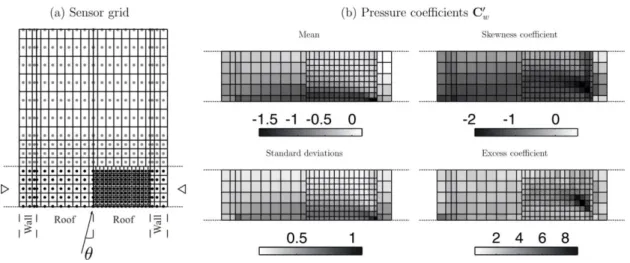
The roof is supported by 11 fixed-base frames spaced every 5.72 m. The first internal structural frame is analyzed and its position is identified with triangles in Figure 1-(a), which is an exploded view of the tap array on the building’s exterior envelope (without the sensors on the gable end). Sensors identified with gray in Figure 1-(a) do not produce forces on the considered frame for analysis and are therefore disregarded.

Figure 1. (a) Exploded view of the tap array with varying tap density on the vertical faces along the length and the roof. The wind angle convention is given: a 0 ° direction corresponds to a wind blowing perpendicularly to the gable end. The triangles identify the frame considered for structural analysis. (b) Maps of mean, standard deviation, skewness and kurtosis coefficients for the pressure coefficients.

The 340° wind direction is chosen for illustration. For convenience, the pressure coefficient is used for illustrations of the random aerodynamic pressures and for the ESWLs defined as

w

C

)

5

.

0

1

(

₂

V

w



_

(11)

where





1

.

225

kg/m³ and

V

is the mean wind speed at eave height in the freestream. Figure 1-(b) shows the maps of the mean and standard deviations along with the skewness and excess coefficients for the pressure coefficients. The aerodynamic pressure field on the right part of the roof exhibits large skewness and excess coefficients that must be taken into account with a non-Gaussian analysis.

The aerodynamic pressure field acting on the cladding is transferred by the girts and purlins to each frame of the building, (details of the finite element model will be given in the full length paper). One structural response, the bending moments at the node identified in Fig. 2-(a) is considered to illustrate ESWLs. Figure 2-(b) illustrates the envelope of bending moments in the frame which is asymmetric. The mean largest maxima of the considered bending moment is equal to 22.03 kNm, as indicated in Figure 2-(b). The dash next to label 41 kNm indicates the scale for the drawing.

Figure 2. (a) Elevation of the considered frame, the dots identify the nodes of the finite element. The bending moment at the node identified by the circle is considered for the computation of ESWLs. (b) Envelope for the bending moments.

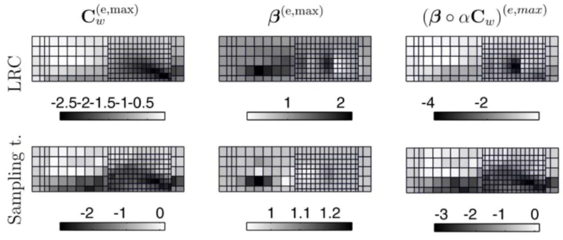
Figure 3 illustrates the ESWLs associated with the mean largest maxima of the considered response. They are obtained with the LRC (top) or Conditional sampling technique (bottom). Original ESWLs are illustrated on the left, load scaling coefficients in the middle and adjusted ESWLs on the right. The coefficient



_i(e,max) is necessary for the ESWL computed with conditional sampling technique and is equal to 1.16. The two methods produce original ESWL which have relatively similar patterns (see left column) but with slight differences in magnitude. The coefficients

β

(e,_i max) for the ESWL computed with the LRC method have a large range of variation [0.23;2.21] in comparison with the conditional sampling technique [0.92;1.28]. For the LRC method, this produces an adjusted ESWL which is no longer close to the original one.

Figure 3. Equivalent static wind loads for the mean largest maxima of the considered bending moment.

5 CONCLUSIONS

Adjusted formulations of an ESWL for structures with quasi-static behaviour and subjected to non-Gaussian aerodynamic pressures have been studied. Two methods have been considered: the conditional sampling pressure technique and the load-response-correlation method. First of all, two properties have been formulated: the envelope value and non-overestimation conditions as important features of an ESWL. Indeed, it appears that the ESWLs may not naturally satisfy these two conditions. In this sense, a 2-step procedure is proposed to rectify original ESWLs, if necessary.

It has been illustrated that the LRC approach may encounter some difficulties in satisfying the non-overestimation condition, i.e., the original ESWL has to be significantly distorted in order to fulfil this condition. In such cases, the authors do not recommend the use of those adjusted ESWLs, as is.

By contrast, it appears that the sampling technique is well suited because the formulation is able to satisfy the non-overestimation condition without much distorsion of the original ESWL, i.e., adjusted ESWLs remain similar to the original ones.

REFERENCES

[1] N. Blaise and V. Denoël, Principal static wind loads, Journal of Wind Engineering and Industrial Aerodynamics 113, 29–39, 2013.

[2] J.D. Holmes, Distribution of peak wind loads on a low-rise building, Journal Of Wind Engineering and Industrial Aerodynamics 29, 59–67, 1988. [3] C. Atta, Sampling techniques in turbulence measurements, Annual Review of Fluid Mechanics 6, 75–91, 1974.

[4] M. Kasperski, Extreme wind load distributions for linear and nonlinear design. Engineering Structures 14, 27–34, 1992.

[5] Y. Tamura, H. Kikuchi and K. Hibi, Actual extreme pressure distributions and lrc formula, Journal of Wind Engineering and Industrial Aero- dynamics 90, 1959–1971, 2002.

[6] S.R. Winterstein, Nonlinear vibration models for extremes and fatigue, Journal of Engineering Mechanics 114, 1772–1790, 1988. [7] A. Kareem and J. Zhao, Analysis of non-gaussian surge response of tension leg platforms under wind loads, Journal of Offshore Mechanics