Shedding Light on the b to s Anomalies
Texte intégral
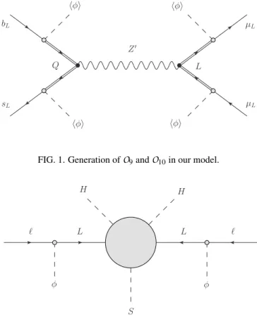
Figure
Documents relatifs
The discrimination between the b → ` and b → c → ` processes is good enough to allow a simultaneous measurement of their branching ratios with the heavy flavour asymmetries. If
In this paper we developed a general framework for relating formal and computational models for generic encryption schemes in the random oracle model.. We proposed general
Since, when the pointwise sum is maximal monotone, the extended sum and the pointwise sum coincides, the proposed algorithm will subsume the classical Passty scheme and
L’archive ouverte pluridisciplinaire HAL, est destinée au dépôt et à la diffusion de documents scientifiques de niveau recherche, publiés ou non, émanant des
are smaller than one, otherwise these are close to one. Red points show the multi-jet background normalization parameters, these are freely floating in the fit and have a core-fit
In particular, it is argued that the failure of the FLEX approximation to reproduce the pseudogap and the precursors AFM bands in the weak coupling regime and the Hubbard bands in
We will then proceed to rewrite this new method in terms of an empirical formula that depends on the running of the fine-structure constant on the Q scale, charge and lepton
L’archive ouverte pluridisciplinaire HAL, est destinée au dépôt et à la diffusion de documents scientifiques de niveau recherche, publiés ou non, émanant des
