The young massive SMC cluster NGC 330 seen by MUSE. I. Observations and stellar content

November 12, 2019

The young massive SMC cluster NGC 330 seen by MUSE.

?

I. Observations and stellar content

J. Bodensteiner

, H. Sana

, L. Mahy

, L. R. Patrick

, A. de Koter

, S. E. de Mink

, C. J. Evans

, Y. Götberg

,

N. Langer

, D. J. Lennon

, F. R. N. Schneider

, F. Tramper

1 _{Instituut voor Sterrenkunde, KU Leuven, Celestijnenlaan 200D, 3001 Leuven, Belgium} e-mail: julia.bodensteiner@kuleuven.be

2 _{Instituto de Astrofísica de Canarias, E-38205 La Laguna, Tenerife, Spain}

3 _{Universidad de La Laguna, Dpto. Astrofísica, E-38206 La Laguna, Tenerife, Spain}

4 _{Astronomical Institute Anton Pannekoek, Amsterdam University, Science Park 904, 1098 XH, Amsterdam, The Netherlands} 5 _{Center for Astrophysics, Harvard & Smithsonian, 60 Garden Street, Cambridge, MA 02138, USA}

6 _{UK Astronomy Technology Centre, Royal Observatory, Blackford Hill, Edinburgh, EH9 3HJ, UK}

7 _{The observatories of the Carnegie institution for science, 813 Santa Barbara St., Pasadena, CA 91101, USA} 8 _{Argelander-Institut für Astronomie, Universität Bonn, Auf dem Hügel 71, 53121 Bonn, Germany}

9 _{Heidelberger Institut für Theoretische Studien, Schloss-Wolfsbrunnenweg 35, 69118 Heidelberg, Germany}

10 _{Institute for Astronomy, Astrophysics, Space Applications & Remote Sensing, National Observatory of Athens, P. Penteli, 15236} Athens, Greece

Received 19 September 2019; accepted 6 November 2019

ABSTRACT

Context.A majority of massive stars are part of binary systems, a large fraction of which will inevitably interact during their lives. Binary-interaction products (BiPs), i.e. stars affected by such interaction, are expected to be commonly present in stellar populations. BiPs are thus a crucial ingredient in the understanding of stellar evolution.

Aims.We aim to identify and characterize a statistically significant sample of BiPs by studying clusters of 10 − 40 Myr, an age at which binary population models predict the abundance of BiPs to be highest. One example of such a cluster is NGC 330 in the Small Magellanic Cloud.

Methods.Using MUSE WFM-AO observations of NGC 330, we resolve the dense cluster core for the first time and are able to extract spectra of its entire massive star population. We develop an automated spectral classification scheme based on the equivalent widths of spectral lines in the red part of the spectrum.

Results.We characterize the massive star content of the core of NGC 330 which contains more than 200 B stars, two O stars, 6 A-type supergiants and 11 red supergiants. We find a lower limit on the Be star fraction of 32 ± 3% in the whole sample. It increases to at least 46 ± 10% when only considering stars brighter than V= 17 mag. We estimate an age of the cluster core between 35 and 40 Myr and a total cluster mass of 88+17₋₁₈× 103_M

.

Conclusions.We find that the population in the cluster core is different than the population in the outskirts: while the stellar content

in the core appears to be older than the stars in the outskirts, the Be star fraction and the observed binary fraction are significantly higher. Furthermore, we detect several BiP candidates that will be subject of future studies.

Key words. stars: massive, emission-line - binaries: spectroscopic - blue stragglers - open clusters and associations: individual: NGC 330 - (Galaxies:) Magellanic Clouds

1. Introduction

Massive stars, i.e. stars with birth masses larger than 8M, have

played a major role throughout the history of the Universe (Jamet et al. 2004; Bresolin et al. 2008; Aoki et al. 2014). Despite their low numbers and short lifetimes, they have a large impact on their environment. They heat, shape and enrich their surround-ings with their high temperatures and luminosities, strong stellar winds, and final explosions (Bromm et al. 2009; De Rossi et al. 2010). Massive stars can evolve following a diversity of evolu-tionary channels. Which channel a star follows depends most significantly on its initial mass, metallicity, rotation, and multi-plicity.

? _{Based on observations collected at the ESO Paranal observatory} under ESO program 60.A-9183(A).

Recent observations have shown that a vast majority of massive stars do not evolve as single stars (see e.g., Sana et al. 2012; Kob-ulnicky et al. 2014; Dunstall et al. 2015). In contrast, they reside in binary systems and will, at some point in their lives, interact with a nearby companion (Sana et al. 2012). Besides stable mass transfer in terms of Roche-lobe overflow, more dramatic inter-actions such as common-envelope evolution and stellar merg-ers are possible (Taam & Sandquist 2000; de Mink et al. 2014; Kochanek et al. 2019). In any of these cases, the star’s mass and angular momentum change significantly which will drastically alter the evolutionary path of the two stars (Podsiadlowski et al. 1992; Vanbeveren & De Loore 1994). Understanding the de-tailed evolution of massive stars, taking into account the effect of multiplicity, remains one of the biggest challenges in modern astrophysics (Langer 2012).

One possible line of investigation in order to explore the effect of multiplicity on the evolution of massive stars is to study stars af-ter they have inaf-teracted, i.e. binary-inaf-teraction products (BiPs). Indeed, the outcome of the interaction process, which defines the physical properties of such BiPs, remains ill-constrained. Char-acterizing the physical properties of BiPs is, however, crucial to assess their current impact on their surroundings and predict their future evolution. This in turn defines the nature and quan-tity of key end-of-life products, such as supernova types and the strength of supernova kicks, the nature and multiplicity prop-erties of compact objects, and ultimately, those of gravitational wave events.

BiPs can be identified through various stellar properties, unfortu-nately none of which ensure an unambiguous identification. Due to the transfer of angular momentum, mass gainers or merger products may be expected to be rapidly rotating (de Mink et al. 2013, Mahy et al. 2019, subm.). The transfer of mass may lead to abnormal chemical abundances on the stellar surface (de Mink et al. 2007; Langer 2012). The supernova explosion of the more massive star can disrupt the system, turning the secondary into a so-called runaway star, a star moving away from its birth place with a high space velocity (Gies & Bolton 1986; Blaauw 1993; Hoogerwerf et al. 2001). If the system remains bound, an excess in UV or hard X-ray flux may indicate the presence of a com-pact companion like in the case of subdwarf companions (see e.g. Gies et al. 1998; Wang et al. 2017, 2018) and X-ray bi-naries (Verbunt 1993; Reig 2011). In star clusters, mass-gainers and mergers are expected to appear younger than their sibling stars, i.e. they are bluer and hotter than the main-sequence turn-off and are massive analogs to the Blue Stragglers found in glob-ular clusters (see e.g., Sandage 1953; Shara et al. 1997; Ferraro et al. 1997; Schneider et al. 2015). Recently, their cooler equiv-alent was proposed by Britavskiy et al. (2019) and Beasor et al. (2019): so-called Red Stragglers, i.e. red supergiants (RSGs) that are more massive and luminous than expected from single-star evolution.

Next to the study of the well-known post-mass transfer Algol systems, searches for BiPs were conducted in several manners in the past: numerous photometric studies found Blue Stragglers in all types of star clusters (see e.g., Ferraro et al. 1997; Ahumada & Lapasset 2007; Gosnell et al. 2014). Schneider et al. (2014) reported indications for BiP signatures in the mass function of young clusters while Ramírez-Agudelo et al. (2013, 2015) found a significant proportion of fast rotators in the presumably single O-type stars in 30 Dor. The relative fraction of these were com-patible with population synthesis predictions of BiPs (de Mink et al. 2013, 2014). The search for BiPs was extended to mag-netic stars through the Binary and Magnetism survey (BinaM-IcS, Alecian et al. 2015; Schneider et al. 2016). Bodensteiner et al. (2018) proposed to use infrared nebulae around massive stars possibly formed in previous binary interactions as general tracers for BiPs.

Population synthesis simulations show that the relative contribu-tions of BiPs to the lower mass content of the cluster vary as a function of age, and peak between 8−40 Myrs, assuming a single starburst (Schneider et al. 2015). While much effort has been in-vested in spectroscopically characterizing the massive star con-tent of young massive star clusters (see e.g., Evans et al. 2011; Sana & Evans 2011; Clark et al. 2014; Ramírez-Tannus et al. 2018, and references therein), these slightly older populations have been relatively overlooked.

Here we aim to investigate the massive star population of the young open star cluster NGC 330. This cluster is situated in the Small Magellanic Cloud (SMC) at a distance of 60 ± 1 kpc

(Har-ries et al. 2003; Hilditch et al. 2005; Deb & Singh 2010). Age es-timates of NGC 330 vary between 26 and 45 Myrs, thus putting it in the age range of interest for our purposes (Sirianni et al. 2002; Martayan et al. 2007b; Milone et al. 2018, Patrick et al., subm.). The estimated photometric mass of NGC 330 ranges be-tween Mphot≈ 3.6×104M(McLaughlin & van der Marel 2005)

and Mphot ≈ 3.8 × 104M(Mackey & Gilmore 2002) which is

in good agreement with a recent estimate of the dynamical mass Mdyn= 15.8+7.6_−5.1× 104M(Patrick et al., subm.).

Several spectroscopic studies of the brightest stars in NGC 330 were conducted in the past reporting a high Be star fraction of about 50% or higher (Feast 1972; Grebel et al. 1992; Lennon et al. 1993; Grebel et al. 1996; Mazzali et al. 1996; Keller & Bessell 1998; Keller et al. 1999). Based on these findings, Maeder et al. (1999) concluded that the Be star fraction in the SMC is higher than the Large Magellanic Cloud and in the Milky Way. A high Be star fraction in SMC clusters (excluding NGC 330) was confirmed by Martayan et al. (2007b). Around 150 OB stars situated in the outskirts of NGC 330 were studied spectroscopically (Evans et al. 2006). Additionally, the cluster was recently investigated by Milone et al. (2018) using Hubble Space Telescope (HST) photometry. The dense cluster core con-taining more than 100 massive stars could not be resolved with existing spectroscopic instrumentation. It is, however, the region where, apart from runaways, many of the massive BiPs are ex-pected due to mass segregation, be it primordial (Sirianni et al. 2002) or as a result of cluster dynamics (Portegies Zwart et al. 2010).

In this first paper of a series, we report on a spectroscopic study of the core of NGC 330 with the Multi-Unit Spectroscopic Ex-plorer (MUSE) mounted at the VLT/UT4 (Bacon et al. 2010). With its capabilities enhanced with adaptive optics (AO), it is now possible to efficiently obtain spectroscopy of individual stars in the dense cluster core. This first paper focuses on the methodology for spectral extraction and on the stellar content of the cluster. Future papers will address multiplicity and physical properties of the stars in the cluster. In Sect. 2 we summarize the observations and the data reduction. Sect. 3 describes the auto-matic routine we develop to extract spectra of stars brighter than V = 18.5 mag. In Sect. 4 we explain how to automatically de-termine spectral types based on the equivalent widths of certain spectral lines between 4600 Å and 9300Å. We present the stellar content of the cluster core in Sect. 5 and compare it to previ-ous photometric and spectroscopic studies of the cluster. Sect. 6 gives a summary and conclusions.

2. Observations and Data Reduction

2.1. Observations with MUSE-WFM-AO

NGC 330 was observed with MUSE on November 19th_{, 2018,}

at Yepun, one of the four Unit Telescopes of the Very Large Telescope (VLT) in Paranal, Chile. MUSE is an integral field spectrograph comprising 24 individual spectrographs.

In wide-field mode (WFM), the 24 individual spectrographs sample a Field of View (FoV) of 1’×1’ with a spatial sampling of 0.2” in both directions. The seeing during the observations varied between 0.4" and 0.7". With the new AO, the MUSE-WFM observations are supported by ground-layer adaptive optics (GLAO) consisting of a deformable secondary mirror, four sodium laser guide stars and the Ground Atmospheric Layer Adaptive OptiCs for Spectroscopic Imaging (GALACSI) module. The observations were carried out in the extended wavelength mode covering a broad optical range (i.e. 4600Å

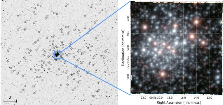
Fig. 1. Left: Finding chart from Evans et al. (2006), where stars that were studied are marked with black circles and the FoV of MUSE is indicated in blue. Right: True color image created by convolving the MUSE data with a B, V, and I filter. At the distance of NGC 330, the size of the FoV of 1’×1’ corresponds to ∼ 20 × 20 pc.

– 9300Å). When supported by AO, the region between 5780 and 5990 Å is blocked by a notch filter in order to avoid light contamination by the sodium lasers of the AO system. The spectral resolving power ranges from 2000 at 4600Å to 4000 at 9300Å.

Five dither positions (DPs) of 540 seconds each were obtained with a relative spatial offset of about 0.7”. The instrument derotator was offset by 90◦ _{after each DP so that the light of}

each star was dispersed by multiple spectrographs. Directly after the observation of NGC 330 an offset sky observation for sky subtraction was taken (see Sect. 2.3). A comparison between the finding chart of Evans et al. (2006) and a true color image showing the spatial coverage of the MUSE observations is shown in Fig. 1.

2.2. Data reduction

The MUSE data were reduced with the standard ESO MUSE pipeline v2.61. The calibrations for each individual IFU included bias and dark subtraction, flat fielding, wavelength and illumina-tion correcillumina-tion. After re-combining the data from each IFU to the merged data cube, a telluric correction and a flux calibration was performed with the help of a standard star observation. Fur-thermore the sky was subtracted in different manners to obtain the best possible result (see Sect. 2.3). The output of the data reduction is a so-called 3D data cube containing two spatial and one spectral direction of dimensions 321 × 320 × 3701. This can either be thought of as 3701 monochromatic images, or about 105_{individual spectra.}

In previous versions of the ESO MUSE pipeline (up to v2.4.1) large-scale (i.e. about 50Å wide) wiggles dominated the blue part of the spectrum when using the MUSE-WFM-AO setup.

1

https://www.eso.org/sci/software/pipelines/muse/

While this problem was fixed in the data extension itself in v2.6, it still occurs in the variance of the reduced MUSE data.

2.3. Sky subtraction

There are different methods to subtract the sky in the ESO MUSE pipeline. As described in Sect. 2.1, an offset sky expo-sure was taken at the end of the observational sequence. It is supposed to be centered on an effectively empty sky region but close to the target region. This facilitates the detection of a dark patch of sky that is not contaminated by stars in order to deter-mine an average sky spectrum. While this procedure works well for isolated objects like galaxies, in the case of NGC 330, which is situated in a dense region of the SMC, it is difficult to find a nearby empty region. In this case, the sky observation is only 3’ away of the science observation and is equally crowded by SMC stars so that the benefits of the sky observation are limited. Extensive testing showed that the remaining sky residuals are smaller when estimating the sky background from the science observations themselves. The MUSE pipeline offers the required framework in which a fraction of the darkest pixels in the science observation is used to estimate an average sky spectrum. This is then subtracted from the science data. The advantage of this method in comparison to using the sky cube is that the average sky spectrum is taken at exactly the same time and thus under the exact same weather and atmosphere conditions.

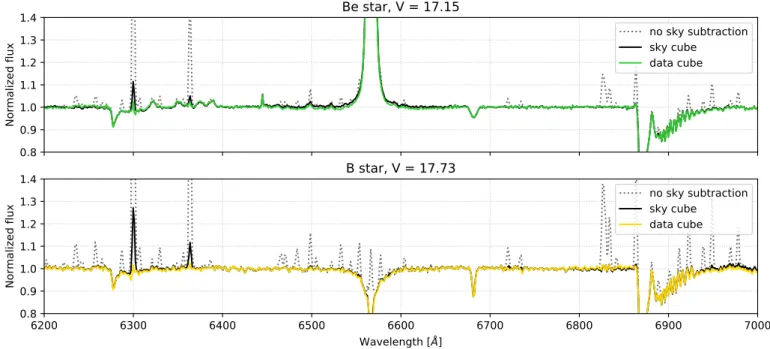
A comparison between the two different sky subtraction meth-ods for a bright star (top panel) and a faint star (bottom panel) is shown in Fig. 2. The figure illustrates that (1) sky subtraction is an important task in the data reduction, and (2) that the residual sky emission lines are smaller using the data cube rather than using the sky cube (see e.g. at λλ 6300, 6365 Å).

0.8

0.9

1.0

1.1

1.2

1.3

1.4

Normalized flux

Be star, V = 17.15

no sky subtraction

sky cube

data cube

6200

6300

6400

6500

6600

6700

6800

6900

7000

Wavelength [Å]

0.8

0.9

1.0

1.1

1.2

1.3

1.4

Normalized flux

B star, V = 17.73

no sky subtraction

sky cube

data cube

Fig. 2. Comparison of the sky subtraction methods for two example stars (marked in Fig. 5 with the corresponding colors). The top panel gives the spectra of an example bright star (#51, a Be star with V = 17.15 mag) and the bottom panel gives those of a fainter star (#33, a B star with V = 17.51 mag). For both stars the original spectrum without any sky subtraction (no sky subtraction), the spectrum with the sky subtraction deduced from the dedicated sky cube (sky cube), and the spectrum with the sky subtraction determined in the science data cube (data cube) are shown. The spectra are not corrected for telluric lines (see e.g. the region between 6850 and 7000 Å).

3. Extraction of stellar spectra

3.1. Targets input catalog

To extract spectra from the MUSE data, we require an input list of stars including stellar positions and brightnesses. We adopt a magnitude cut at V = 18.5 mag which approximately corre-sponds to 6Mat SMC distance and extinction. This results in

a signal-to-noise ratio (S/N) of around 80 which is high enough for our further analysis.

Accurate stellar positions can be estimated in the MUSE data directly. They are, however, preferably determined from an in-strument of higher spatial resolution, the Hubble Space Tele-scope (HST), providing an approximately ten times better spa-tial resolution. The core of NGC 330 was observed with WFPC2 and the F555W filter (approximately corresponding to the V-band) in 1999, and with WFPC3 and the F336W filter (approxi-mately corresponding to the U-band) in 2015. Unfortunately, the F555W filter image does not cover the full MUSE FoV (see Fig. 3). The F336W data cover the whole FoV but the filter is outside the wavelength range covered by MUSE. For both images, an automatically created source list based on DAOphot is available on the HST archive2_{. The brightest stars (i.e. stars brighter than}

V < 15 mag) are saturated in the HST images and thus missing from the input list.

As can be seen in Fig. 3, the coordinate systems in both HST input catalogs are not aligned with the MUSE world coordinate system (WCS). We thus first align the two HST catalogs with each other, and in a subsequent step with the MUSE WCS. For this, we pick a handful of isolated stars in the MUSE image, de-termine their positions by fitting a point-spread function (PSF), and then compute the coordinate transformation between these known sources in MUSE and in the aligned HST catalogs. The coordinate transformation from the HST coordinate system (x’,

2

https://archive.stsci.edu/hst/

y’) into the MUSE coordinate system (x, y) is given by:

x= +x0· cos(θ)+ y0· sin(θ)+ ∆x (1) y= −x0· sin(θ)+ y0· cos(θ)+ ∆y (2)

The best-fit values derived for the coordinate transformation are ∆x = (1.79 ± 0.36) px, ∆y = (1.06 ± 0.43) px, and θ = (−0.05 ± 0.10)◦_{. This transformation is applied to all HST}

sources.

To obtain a complete target list containing V magnitudes of all stars we combine the F336W and the F555W list. We use stars appearing in both lists and brigther than 19.5 in F555W to com-pute a correlation between F555W magnitudes and F336W mag-nitudes. This allows us to approximately convert F336 magni-tudes in F555W magnimagni-tudes for stars which are not covered by the F555W data (see Fig. 3 and 4). This conversion is only ac-curate for early type main-sequence stars, for which the U-band filter covers the Rayleigh-Jeans tail of the spectrum. It does not hold for stars that are evolved off the main sequence (MS), e.g. for RSGs and blue supergiants (BSGs). As mentioned above, given the brightness of these stars, they are saturated in the HST images. For the same reason they have, on the other hand, been previously studied (see e.g. Arp 1959; Robertson 1974; Grebel et al. 1996). We thus adopt their V-band magnitudes from Robertson (1974) when available (see Tab. 2).

The final target list is constructed by taking all sources that are within the MUSE field of view and brighter than V= 18.5 mag. Seven stars that are clearly brighter than V= 18.5 mag are miss-ing in both HST input lists. This is probably due to problems in the automated source finding routines. These seven stars are added manually before constructing the final target list which contains 278 stars.

0

50

100

150

200

250

300

x coordinate [px]

0

50

100

150

200

250

300

y coordinate [px]

Fig. 3. HST source positions overlaid over an integrated-light image extracted from the MUSE cube. Stars with only F336W magnitudes are marked in pink while stars with only F555W magnitudes are marked in blue. Stars which appear in both lists and are brigther than 19.5 in F555W are marked in green. The latter ones are used to determine a cor-relation between the two magnitudes (see Fig. 4). The two HST source catalogs need to be aligned with respect to the MUSE coordinate sys-tem by shifting them by∆x = (1.79 ± 0.36) px and ∆y = (1.06 ± 0.43) px, and rotating them by θ= (−0.05 ± 0.10)◦

. 15.5 16.0 16.5 17.0 17.5 18.0 18.5 19.0 19.5 20.0 F336W mag 15 16 17 18 19 20 F555W mag

used for correlation fit not used for correlation fit correlation

Fig. 4. Correlation between the HST F336W (∼ U-band) and F555W (∼ V-band) magnitudes. In order to fit the linear correlation (green line) we exclude stars with F555W fainter than 19.5 (see Sec. 3.1) and brighter than 16.5 (gray regions). Stars that are brighter in F555W but not in the UV are RSGs and thus not included in the fit. The relation is used to convert F336W magnitudes to F555W magnitudes for all stars in the HST input catalogs. The grey dotted line indicates the one-to-one relation.

3.2. Source extraction

The high source density especially in the center of the image and the associated spatial overlap of sources makes extracting stel-lar spectra a complicated task. Given the format of the reduced MUSE data (i.e., a 3D data cube with two spatial and one

spec-0

50

100

150

200

250

300

x coordinate [px]

0

50

100

150

200

250

300

y coordinate [px]

Fig. 5. Stars contained in the final target list (i.e. stars brigther than 18.5 in F555W) overplotted in orange over the MUSE white light image. The size of the circle corresponds to their inferred brightness in the V-band. The stars marked with orange filled circles are used to fit the PSF (see Sect. 3.2). The spectra of the stars marked with red, blue, green, and yellow filled circles are shown in Fig. 6.

tral dimension), obtaining a spectrum of a source is equivalent to measuring its brightness in each wavelength image (referred to as a slice in the following). We avoid simple aperture photome-try (i.e. adding up the flux in a given aperture around each star’s position) in each slice because of the crowding of the field. We develop our own spectral extraction routine that employs PSF fitting. The routine is mainly based on the python package photutils (Bradley et al. 2019), a translation of DAOphot (Stet-son 1987) into python, which provides a framework for PSF fit-ting in crowded fields. We use the input list described in Sect. 3.1 containing the 278 brightest stars. Subsequently, an effective PSF model (Anderson & King 2000) is derived from a selected set of isolated stars (see Fig. 5). Slice by slice (i.e. wavelength by wavelength), this PSF model is fitted to each source, while the positions taken from the input list are held fixed. In this way, we determine the total flux and flux error of a given star in each slice. All fluxes and error values for each star are then concate-nated to a spectrum.

Crowding of the field is taken into account by simultaneously fitting the PSF of stars that are closer together than 12 pixels (corresponding to 2.4"). An example of the extraction of spec-tra for deblended sources is shown in Appendix A. For seven stars the extraction of a spectrum was not possible due to severe crowding. In total we extract spectra for 271 stars brighter than V= 18.5 mag.

3.3. Normalization

After automatically extracting the spectra of the brightest stars we normalize them in an automatic manner. The normalization is performed for all spectra save for those of RSGs which require special treatment in account of the large number of spectral lines. To normalize the spectra, the continuum has to be determined

5000

5500

6000

6500

7000

7500

8000

8500

9000

Wavelength [Å]

Arbitrary Flux

He I H He I

He II

H He I

He I

O I

H

V = 13.76 RSG

Na I filter

V = 13.18 BSG

Na I filter

V = 17.73 B star

Na I filter

V = 17.15 Be star

Na I filter

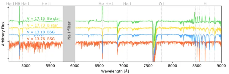
Fig. 6. Example spectra for different stars. From top to bottom: the spectrum of a Be star (green), a B star (yellow), a BSG (blue) and a RSG (red). Our automated normalization mechanism was not applied to the RSG, it was normalized manually. The estimated V-band magnitude is given for each star. Important diagnostic lines are indicated. The gray shaded region indicates the wavelength region blocked by the sodium filter. The spectra are not corrected for tellurics.

and fitted with a polynomial. For this, spectral lines have to be identified and excluded from the fit. This continuum search is based on a two-step process adapted from Sana et al. (2013). First, a minimum-maximum filter and a median filter are com-pared in a sliding window of a given size. If the value in the min-max filter exceeds the value of the median filter by a thresh-old value that depends on the S/N of the spectrum, a spectral line or cosmic hit is detected and the point is excluded from the fit. A polynomial is fit to this preliminary continuum. Points are ex-cluded from the continuum points if they lie further away than a second threshold value from the polynomial fit, and a new poly-nomial is fit through the remaining continuum points. This pro-cedure is repeated in an iterative manner.

We consider the blue and the red part of the spectrum (i.e. wave-lengths below and above the blocked laser-contaminated region between 5780 and 5990 Å) independently. Furthermore, in the wavelength region dominated by the Paschen lines, continuum flux is determined in fixed wavelength windows.

Normalized example spectra for a Be star, a B star, a RSG and a BSG are shown in Fig. 6. The estimated V-band magnitude is indicated in the plot. Using this method we achieve a normal-ization accuracy of around 2.5% for all the spectra. The average S/N is greater than 400 for the BSGs and varies between 300 for the brightest and 80 for the faintest B stars in our sample.

4. Automated spectral classification

4.1. Main sequence stars

Commonly used spectral classification schemes are based on the blue part of the spectrum, i.e. on wavelengths below 4600 Å (Conti & Alschuler 1971; Walborn & Fitzpatrick 1990). Unfor-tunately, this region is not covered by the MUSE extended setup (see Sec. 2.1) and thus standard schemes cannot be applied to our case. Given the large amount of stellar spectra in our dataset we aim for an automated procedure that is reproducible and in-dependent of human interaction.

We develop a new classification scheme for OBA main-sequence stars in the red part of the spectrum that is based on the relation between spectral type and the equivalent width (EW) of spectral lines. Similar approaches were proposed by e.g. Kerton et al. (1999) or Kobulnicky et al. (2012) and applied to MUSE data

5400 5410 5420 1.0 1.5 2.0 2.5 3.0 3.5 4.0 4.5

Arbitrary Flux

He II

Wavelength [Å]

He I

A7

A3

A0

B9

B7

B5

B3

B2.5

B1

B0

O9.5

O9

O8.5

O8

O7.5

O7

O I

Fig. 7. Atlas of spectral standards listed in Tab. 1 around the three lines of interest. The spectra are shifted horizontally according to the radial velocity and vertically for clarity. The black line shows the original spectra while the dotted line indicates the spectra degraded to MUSE resolution.

by Zeidler et al. (2018) and McLeod et al. (2019). While Kerton et al. (1999) focus on earlier spectral types between O5 and B0, Kobulnicky et al. (2012) make use of line ratios including the He I λ 5876 line that is covered by the Na I filter in our data. Their classification can thus not be applied to our case.

We select different diagnostic lines focusing in particular on He II λ 5412, He I λ 6678 and the O I triplet centered around λ 7774. EWs are not altered by stellar rotation or extinction and can be measured in a consistent manner at MUSE resolution.

In order to calibrate the classification scheme we use the stan-dard stars listed in Gray & Corbally (2009). For all stars, ob-servations obtained with the HERMES spectrograph mounted at the Mercator telescope in La Palma (Raskin et al. 2011) are available. HERMES is a high-resolution spectrograph provid-ing spectra with R = 85 000. All classification spectra have a S/N > 150. Because of the lack of late-O and early-B spectral standard stars in Gray & Corbally (2009) we complement the list with the O star spectral atlas by Sana et al. (in prep.). The O star spectra used are observed with the Fibre-fed Extended Range Optical Spectrograph (FEROS, Kaufer et al. 1999) mounted at the 2.2m Max-Planck-ESO telescope in La Silla, Chile which has a resolving power of 48 000. In a handful of cases both HER-MES and FEROS observations are available for the same star. In these cases we use the higher resolution, higher S/N HERMES spectra. All spectra used for the calibration are shown in Fig. 7 as a sequence of spectral type.

An overview of all calibration stars, their spectral types as listed in Gray & Corbally (2009) or Sana et al. (in prep.), and pos-sible additional classifications are listed in Table 1. Some stars show variable spectra. Several are single- or double-lined spec-troscopic binaries or known pulsating stars. After downgrading the spectra to MUSE resolution we inspect the classification spectra to search for obvious contamination caused by the be-fore mentioned variability. In almost all cases these are washed out due to the low resolution. Only ν Ori (B0V) shows a com-posite spectrum typical of a double-lined spectroscopic binary comprising an early type (Teff ≈ 20 000 K) and a later type star

(Teff ≤ 15 000 K). It is thus not further considered in our

classi-fication.

For all the standard stars we measure the EW and the corre-sponding error σEWin a 16Å-wide window w around the center

of the three lines mentioned above. The errors are estimated fol-lowing Chalabaev & Maillard (1983):

σEW =

√

2 · w ·∆λ

S/N (3)

where the S/N is the signal-to-noise ratio of the continuum close to the considered line and∆λ is the wavelength step (i.e. 1.25 Å for MUSE). We use these measured EWs to fit a second degree polynomial giving a relation between EW and spectral type. We repeat the measurements with degraded standard star spectra in which we adopt the resolution of MUSE and apply a typical S/N to the standard star data. While the relations themselves do not change, we use these measurements to investigate the limit for which genuine spectral lines can be distinguished from noise in the continuum. Given our data quality, this limit is 0.1 Å. EW values are only considered for the relation fit if they are larger than this limit. Figure 8 shows the relations between EWs and spectral type for all three considered lines.

A special case is the He II line at 5412 Å. In late-type stars (i.e. A3 and later) metal lines start to dominate in the considered wavelength regime and especially the Fe I (λ 5410.9 Å) and the Ne I line (λ 5412.6Å) contribute to EW measurements (marked with blue triangles Fig. 8). We thus exclude these points from the relation fit at late spectral type.

The derived relations between a fractional spectral type (xSpt)

O7 O9 B1 B3 B5 B7 B9 A1 A3 A5 A7 0.0 0.2 0.4 0.6 0.8 1.0 Eq uiv ale nt w idt h [Å ] _{He II 5412 Å} O7 O9 B1 B3 B5 B7 B9 A1 A3 A5 A7 0.0 0.2 0.4 0.6 0.8 1.0 Eq uiv ale nt w idt h [Å ] _{He I 6678 Å} standard used standard O7 O9 B1 B3 B5 B7 B9 A1 A3 A5 A7 Spectral type 0.0 0.2 0.4 0.6 0.8 1.0 Eq uiv ale nt w idt h [Å ] _{O I 7774 Å}

Fig. 8. From top to bottom: Correlation between equivalent width mea-sured in the standard star spectra and their spectral type for He II λ 5412, He I λ 6678 and the O I triplet at λ 7774. Black dots show the measured values while black crosses indicate the data points used to fit the poly-nomial. EW measurements below 0.1Å (shaded region around the black line at 0 Å) do not allow a significant detection of spectral lines from noise in the continuum and are thus excluded from the fit. In the spe-cial case of the He II line the EWs at late spectral types (A5 and later), which are contaminated by metallic lines and thus not considered in the fit, are indicated by blue triangles.

and the EW in Å for the considered lines are: xSpt= − 0.4402 − √0.3215 − 0.3905 · EW5412 0.1952 ; xSpt∈ [−3, 0] (4) xSpt= − 0.0360 − √0.0152 − 0.0195 · EW6678 0.0098 ; xSpt∈ [−3, 9] (5) xSpt= + 0.0809 − √0.0075 − 0.0096 · EW7774 0.0048 ; xSpt∈ [0, 17] (6) in which we consider a linear translation of spectral type to xSpt

where B0 corresponds to xSpt= 0 and B9 to xSpt= 9.

Figure 8 shows these results graphically: the differentiation be-tween early B- and late O-type stars is per definition the presence of significant He II lines. The EW of the He II line at 5412 Å can thus be used as classifier for the presence of O stars in our sample. As He I lines are present in late O- to late B-type stars, our second relation can be extrapolated to spectral type B9 and thus be used for stars O7-B9. Finally, the O triplet at 7774 Å is present in spectral types later than B3 (up to A7).

The derived relations are based on the standard star spectra of galactic stars and are not corrected for the effect of metallicity. As NGC 330 is in the SMC, i.e. at significantly lower metallic-ity, the O I line is weaker in our sample than predicted by the galactic standard stars. As the effect of metallicity is negligible for the He I and He II lines, we focus on those lines to determine spectral types in the MUSE data.

The strength of the O I triplet at λ 7774 is sensitive to temper-atures covered by later spectral types, i.e. especially to A-type stars where the He I λ 6678 line is not present anymore. In order

Table 1. OBA spectral standards from Gray & Corbally (2009) and Sana et al. (in prep.). The radial velocities (col. 3) and additional information (col. 4) are taken from references indicated in col. 5. Stars marked with a † are listed in Sana et al. (in prep.). The top part of the table gives main sequence standard stars (see Sec. 4.1) while the bottom part gives giant and supergiant standards (see Sec. 4.2).

Classification Identifier vrad Additional information References [km/s]

O7V 15 Mon 22.0 Oe star, SB2 (O7Ve+ O9.5n) Gies et al. (1993)

O7.5Vz † HD 152590 0.0 eclipsing binary, SB2 Sota et al. (2014), Sana et al. (in prep.)

O8V † HD 97848 - 7.0 - Walborn (1982), Sota et al. (2014), Sana et al. (in prep.) O8.5V HD 46149 45.9 SB2 (O8.5V+ B0-1V) Mahy et al. (2009), Sana et al. (in prep.)

O9V 10 Lac -10.1 - Sota et al. (2011)

O9.5V † HD 46202 53.0 Sota et al. (2011), Sana et al. (in prep.)

B0.2V † τ Sco 2.0 magnetic star Donati et al. (2006)

B1V † ω Sco - 4.4 variable star of β Cep type Telting & Schrijvers (1998), Sana et al. (in prep.)

B2.5V(n) † 22 Sco 0.0 - Bragança et al. (2012), Sana et al. (in prep.)

B3V η Aur 7.3 - Morgan & Keenan (1973)

B5V HD 36936 18.7 - Schild & Chaffee (1971)

B7V HR 1029 - 1.5 pulsating variable star Grenier et al. (1999); Szewczuk & Daszy´nska-Daszkiewicz (2015)

B9V HR 749A 9.7 - Gray & Corbally (2009)

A0Va α Lyr - 20.6 variable star of δ Sct type Gray et al. (2003); Böhm et al. (2012)

A3V β Leo - 0.2 variable star of δ Sct type van Belle & von Braun (2009); Bartolini et al. (1981) A7V HR 3974 - 11.4 variable star of δ Sct type Gray et al. (2003); Rodriguez et al. (1991)

A0 Ia HR 1040 - 6.2 evolved supergiant star Bouw (1981); Gray & Garrison (1987)

A0 Ib η Leo 1.4 - Cowley et al. (1969); Lobel et al. (1992)

A0 III α Dra - 13.0 SB1 Cowley et al. (1969); Levato (1972); Bischoff et al. (2017)

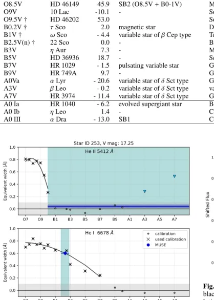
O7 O9 B1 B3 B5 B7 B9 A1 A3 A5 A7 0.0 0.2 0.4 0.6 0.8 1.0 Eq uiv ale nt w idt h [Å ] He II 5412 Å Star ID 253, V mag: 17.25 O7 O9 B1 B3 B5 B7 B9 A1 A3 A5 A7 Spectral type 0.0 0.2 0.4 0.6 0.8 1.0 Eq uiv ale nt w idt h [Å ] He I 6678 Å calibration used calibration MUSE

Fig. 9. EW measurements for star # 253 overplotted over the fit relations described in Equations (4) and (5). As mentioned above, we focus on the He lines to determine the spectral type. The blue shaded region indicates the allowed range of spectral types given the measured EWs with corre-sponding errors. Using this automated method, we determine a spectral type B2 with an accuracy of about one subtype. See also Fig. 10.

to be able to detect possible A-type stars we first classify all stars including the O I line. We do not detect any spectrum only show-ing O I lines and no He I, i.e. there are no A-type main-sequence stars in the sample. The only cases where O I is present in the spectra also show strong He I lines, a signature indicative of the composite spectra of spectroscopic binaries (see Sec. 4.4). The classification using the He II and He I lines is applied to all B-type main-sequence stars and yields fractional spectral types interpolated from the beforementioned relations. Taking into ac-count the errors we achieve an accuracy of around one spectral subtype. An overview over the derived values is given in

Ap-4700 4725 0.0 0.2 0.4 0.6 0.8 1.0 Shifted Flux He I 4900 4925 He I 5400 5425 Wavelength [Å] He II 65506600 H 6675 6700 He I 7750 7775 B1 B2.5 B3 B5 B7 O I

Fig. 10. By-eye classification of star #253. The stellar spectrum (in black) is compared to five standard stars, downgraded to MUSE reso-lution. The continuous lines show the original spectra while the dashed dotted lines show the spectra rotationally broadened by 200 km/s. By eye, the star would be classified as B1-B2 star, which is in agreement with the automatically derived spectral type of B2 ± one subtype. See also Fig. 9.

pendix D. An example diagnostic plot showing the measured EW for one star (#253) and the derived spectral type is given in Fig. 9. For comparison reasons, Fig. 10 shows the classifica-tion of the same star by eye. Both methods agree within their errors.

Due to the difficulty to distinguish dwarf and giant luminosity classes given the low resolution of the MUSE data we derive the automated classification scheme for main-sequence stars only, implicitly assuming that all stars, but supergiants, are on the main sequence. We apply it to all sample stars except supergiants (that are several magnitudes brighter and clearly identifiable in the MUSE data, see Sect. 4.2). Besides RSGs and BSGs, the au-tomatic approach to classification reveals its limitations for Be stars and spectroscopic binaries showing a composite spectrum.

The identification and classification of these stars is described in the following sections.

4.2. Red & blue supergiants

Red and blue supergiants are identified based on their brightness, they are about several magnitudes brighter in the V band than the main sequence stars. We find eleven bright red and six bright blue stars in the cluster core. Focusing on the bright red stars, Lee et al. (in prep.) check cluster membership based on Gaia DR2 proper motion and parallax measurements (Gaia Collabora-tion et al. 2018). They find that four stars have less reliable Gaia data and might be potential Galactic contaminants. Their radial velocities are, however, in good accordance with the SMC radial velocity. Given the large uncertainties in Gaia DR2 parallaxes for the bright blue stars we assess SMC membership by measur-ing their radial velocities, which are all in good agreement with the radial velocity of the SMC. In total, there are eleven RSGs and six BSGs in the cluster core.

In order to verify that the stars are supergiants rather than giants we calculate their absolute V magnitude using the distance mod-ulus m − M= 5 log d −5+ AV, assuming a distance of 60 kpc and

an extinction of E(B − V)= 0.08 (Keller et al. 1999, D. Lennon, priv. comm.). As shown in Tab. 2, the V-band magnitudes of the RSGs and BSGs are between 12.6 and 14.1. This gives absolute magnitudes between -6.5 and -5.0 which is in the range of ex-pected absolute magnitudes for bright A-type giants and A-type supergiants.

The eleven RSGs in NGC 330 are studied in greater detail in Patrick et al. (subm.) who derive spectral types following the classification criteria and methodology detailed in Dorda et al. (2018). We adopt their spectral type classification and include them in Tab. 2.

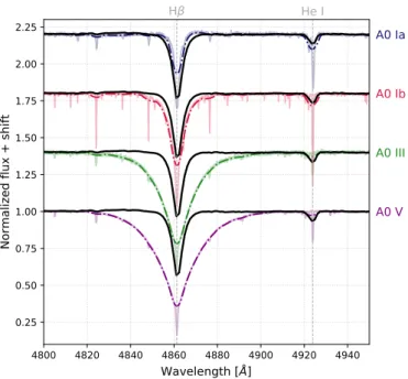
For the classification of the six blue supergiants we use a second set of standard star spectra of different luminosity class from Gray et al. (2003) observed with the HERMES spectrograph. Standard star spectra are available for spectral types B5, A0, and A7 and include luminosity classes Ia, Ib, and III.

When classifying the blue supergiants from the MUSE data, we first determine the spectral type based on He I lines and then esti-mate the luminosity class based on the width of the Balmer lines. As explained above, the strength of metallic lines can not be used for classification due to the lower metallicity of the SMC. Given the availability of the classification spectra we give a wide spec-tral type estimate of late-B, early-A and late-A.

Five of the six blue supergiants are early-A stars while one is a late A-type star. While one star has luminosity class Ia-Ib, all the other supergiants are of luminosity class Ib-III. One example for the spectral classification of an A-type supergiant is shown in Fig. 11.

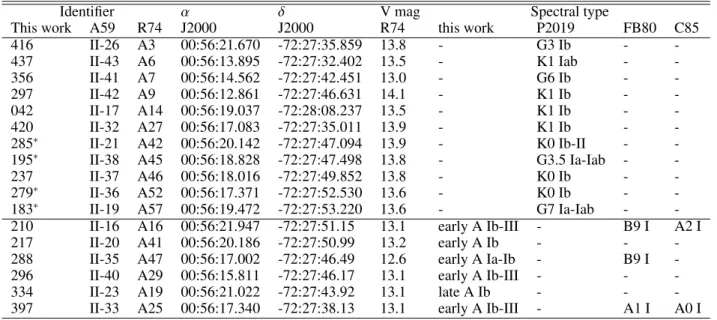
Three of the A-type supergiants have already been studied in pre-vious works by Feast & Black (1980) and Carney et al. (1985). Their spectral types agree with the ones derived in this study within the errors. Two blue supergiants have not been mentioned in literature before. Table 2 gives a summary of all the parame-ters of the RSGs and BSGs derived here compared to literature values.

4.3. Be stars

Classical Be stars are rapidly rotating B-type stars with Balmer lines as well as other spectral lines from e.g., O I and He I in emission, arising from a circumstellar decretion disk (Rivinius

4800 4820 4840 4860 4880 4900 4920 4940

Wavelength [Å]

Normalized flux + shift

H

He I

A0 Ia

A0 Ib

A0 III

A0 V

Fig. 11. Spectral classification of an A-type supergiant (#161). The MUSE spectrum (in black) is compared to four standard star spectra of spectral type A0 Ia, A0 Ib, A0 III, and A0 V. The continuous line shows the original spectra while the dashed dotted lines show the spectra ro-tationally broadened by 200 km/s. All standard star spectra are down-graded in resolution to match the MUSE data. We classify this star as early A-type star with luminosity class Ia-Ib.

et al. 2013). Different possible origins for the rapid rotation of Be stars have been proposed. Be stars could be born as rapid ro-tators (Bodenheimer 1995; Martayan et al. 2007b). They could also become rapid rotators during their MS evolution, either as single stars (Ekström et al. 2008) or due to transfer of mass and angular momentum in a binary system (Packet 1981; Pols et al. 1991; Vanbeveren & Mennekens 2017). The strength of the emission lines is variable on timescales of months to years and strongly depends on the disk density and inclination angle (see e.g. Hanuschik et al. 1988). Next to Hα, the O I λ 7774 line is most strongly affected by the infilling due to disk emission and often appears completely in emission.

For this reason, besides automatically deriving a spectral type from the EW of the He I line, we compare the spectra of all Be stars to standard star spectra of B-type main-sequence stars by eye where a larger focus is put on all available He I lines. We achieve an accuracy with the visual inspection method of up to about 3 spectral subtypes. One example of this method of classi-fication is shown in Appendix B. Both methods agree within the errors for a majority of the stars in the sample. In cases where the methods disagree we keep the spectral type that was derived through visual inspection as it allows us to takes into account more spectral lines.

Both methods, however, are based on the strength of the He I lines which grow in strength with earlier spectral types. As they may suffer from infilling and thus appear less deep than they ac-tually are, a systematic shift in classification towards later spec-tral types is possible. The estimated specspec-tral types are thus a lower limit in terms of spectral type.

In total we find Balmer line emission in 82 of the 251 MS stars in the sample. This gives a lower limit on the observed Be star fraction in our sample of fBe= 32±3%. While most of the

emis-sion line stars are of mid- to late B-type , we find one O9.5eV and one O9.5/B0eV star in the sample. Both stars show clear

ab-Table 2. Overview of the parameters of the red and blue supergiants, both from this paper and from literature.

Identifier α δ V mag Spectral type

This work A59 R74 J2000 J2000 R74 this work P2019 FB80 C85

416 II-26 A3 00:56:21.670 -72:27:35.859 13.8 - G3 Ib - -437 II-43 A6 00:56:13.895 -72:27:32.402 13.5 - K1 Iab - -356 II-41 A7 00:56:14.562 -72:27:42.451 13.0 - G6 Ib - -297 II-42 A9 00:56:12.861 -72:27:46.631 14.1 - K1 Ib - -042 II-17 A14 00:56:19.037 -72:28:08.237 13.5 - K1 Ib - -420 II-32 A27 00:56:17.083 -72:27:35.011 13.9 - K1 Ib -

-285∗ II-21 A42 00:56:20.142 -72:27:47.094 13.9 - K0 Ib-II -

-195∗ _{II-38 A45 00:56:18.828 -72:27:47.498 13.8 - G3.5 Ia-Iab -}

-237 II-37 A46 00:56:18.016 -72:27:49.852 13.8 - K0 Ib -

-279∗ II-36 A52 00:56:17.371 -72:27:52.530 13.6 - K0 Ib -

-183∗ _{II-19 A57 00:56:19.472 -72:27:53.220 13.6 - G7 Ia-Iab -}

-210 II-16 A16 00:56:21.947 -72:27:51.15 13.1 early A Ib-III - B9 I A2 I

217 II-20 A41 00:56:20.186 -72:27:50.99 13.2 early A Ib - -

-288 II-35 A47 00:56:17.002 -72:27:46.49 12.6 early A Ia-Ib - B9 I

-296 II-40 A29 00:56:15.811 -72:27:46.17 13.1 early A Ib-III - -

-334 II-23 A19 00:56:21.022 -72:27:43.92 13.1 late A Ib - -

-397 II-33 A25 00:56:17.340 -72:27:38.13 13.1 early A Ib-III - A1 I A0 I

Notes. Literature identifications are from Arp (1959, A59) and Robertson (1974, R74). Literature spectral types are from Patrick et al. (subm., P2019), Feast & Black (1980, FB80), and Carney et al. (1985, C85).∗

identifies potential Galactic contaminants based on Gaia data.

5400 5425 0.4 0.5 0.6 0.7 0.8 0.9 1.0 1.1

Normalized flux + shift

He II

H

He I

O9

O9.5

B0

O I

Normalized flux + shift

6550 6575 6650 6700

Wavelength [Å]

O9

O9.5

B0

Fig. 12. Spectral classification of the O9.5e star (#147, upper panel) and the O9.5/B0e star (#157, lower panel). The two stellar spectra (in black) are compared to three standard star spectra of spectral type O9, O9.5, and B0 in blue, red, and green (described in Sect. 4.1), downgraded to MUSE resolution. The continuous line shows the original spectra while the dashed dotted line shows the spectra after applying rotational broadening by 200 km/s.

sorption in the He II line at λ 5412. Their spectra are shown in Fig. 12.

4.4. Spectroscopic binaries

As we only consider one epoch in this study, we can not rely on radial velocity variations to detect spectroscopic binaries. Nev-ertheless we find indications for binarity in some of the spectra.

For some stars we see strongly asymmetric lines made up of two line components of different radial velocity. Other spectra appear to be composite spectra showing both deep He I lines indicative of an early spectral type as well as deep O I lines characteristic for a later spectral type.

Composite spectra could also occur when two sources are so close in the plane of the sky that their spectra are extracted to-gether. The spectral extraction using PSF fitting based on the higher spatially resolved HST data as input catalog takes this into account. Other possible explanations of the observed line shapes could be, for example, different micro-/macroturbulence values that affect lines differentially. A higher oxygen abundance could lead to a sronger OI line. A more certain classification as spectroscopic binary will only be possible when periodic radial velocity shifts are detected.

In total, we find 36 candidate spectroscopic binaries in our sam-ple. If there is no false-positive due to the possible reasons men-tioned above, this would imply a lower limit on the observed spectroscopic binary fraction of fbinary = 14 ± 2%. One

exam-ple spectrum is shown in Fig. 13. A more thorough investigation of the spectroscopic binaries will follow in paper II of this se-ries where we will use all available 6 epochs to measure radial velocities for all stars.

5. Stellar content of NGC 330

5.1. Spectral types

Out of the 278 stars brighter than V = 18.5 mag, there are 249 B type stars, two O type stars, eleven RSGs, and six A-type su-pergiants. For seven stars, the extraction of a sufficiently uncon-taminated spectrum was not possible, and three stars appear to be foreground stars. 82 of the main sequence stars show Balmer line emission and are classified as Be stars. A distribution of spectral subtypes for B and Be stars is shown in Fig. 14. Most of the stars are of spectral type B3 to B6. There are only a few stars with spectral type B2 and earlier and only one O-type and one O9/B0 star (both are in fact Oe/Be stars). The lack of later

spec-5400 5425 0.4 0.5 0.6 0.7 0.8 0.9 1.0 1.1

Normalized flux + shift

He II

H

Wavelength [Å]

He I

B0

B5

B9

O I

Fig. 13. Composite spectrum of the spectroscopic binary #8. The spec-trum of the star (in black) is compared to three standard star spectra of spectral type B0, B5, and B9 in blue, red, and green, respectively (described in Sect. 4.1), downgraded in resolution to match the MUSE data. The continuous colored line shows the original spectra while the dashed dotted line shows the spectra after applying rotational broaden-ing by 200 km/s. O7 O8 O9 B0 B1 B2 B3 B4 B5 B6 B7 B8 B9

Spectral type

Counts

Be star fraction [%]

Fig. 14. Distribution of spectral types for main-sequence stars, where yellow indicates B stars and green indicates Be stars. The left axis shows the total number of stars while the right axis indicates the Be star frac-tion in each bin. The accuracy of spectral type determinafrac-tion is about one spectral subtype. Overplotted is the Be star fraction in each bin, for which we give counting errors except for cases where the Be star fraction is 0 or 100%.

tral types, i.e. of late-B and A type stars is probably due to the cut in brightness applied when extracting the spectra (i.e. only stars with V < 18.5 are considered).

The spatial distribution of all stars is shown in Fig. 15. While B-type stars seem to be evenly distributed, the Be stars seem to be clustered in the south-east part of the cluster core (i.e., the lower left corner of the image). Red and blue supergiants are mostly found in the inner region of the cluster.

A handful of stars in our sample were studied by Grebel et al. (1996), Evans et al. (2006), and Martayan et al. (2007a). The two stars studied by Grebel et al. (1996) have similar spectral types but different luminosity classes and were classified as Be

0

₅₆

₂₁

₁₈

₁₅

₁₂

-72°27'30"

45"

28'00"

15"

Right Ascension

Declination

Fig. 15. Stellar classification for all 275 stars with V < 18.5 mag over-plotted over a MUSE RGB image created from the B, V, and I filters. B stars are marked with yellow circles, Be stars with green diamonds, RSGs with red circles and BSGs with blue circles.

stars by them while they show no signs of emission in our spec-tra (#5= Arp II-4 was as B2-3Ve star while we classify it as B3V star; #461= Arp II-31 was classified as B2-3 IIe star while we classify it as B5 V star). This could either be due to the variable nature of the Be star phenomenon, or it could be caused by Hα contamination in the spectra used by Grebel et al. (1996). Our derived spectral types for the two stars scrutinized by Evans et al. (#011= NGC 330-036 and #253 = NGC 330-095), are within the error bars: we classify #011 as B3 while it is listed as B2 II star in Evans et al. (2006), and #253 as B2, which by them is listed as B3 III star.

Furthermore, there are six stars in common with the sample of Martayan et al. (2007a) which are classified as early Be stars (B1e-B3e). For those stars (#53, #88, #140, #166, #456 and #460) we find a systematically later spectral type between B3e and B6e. This systematic difference could be due to their dif-ferent classification methods: while we determine spectral types based on the EW of diagnostic spectral lines and by visual com-parison to standard star spectra, Martayan et al. estimate Teffand

log g from the spectra and transcribe these into spectral types and luminosity classes adopting the galactic calibrations by Gray & Corbally (1994) for B stars, and Zorec et al. (2005) for Be stars.

5.2. Color Magnitude Diagram

We use the HST photometry published in Milone et al. (2018)3

to reconstruct their color magnitude diagram (CMD) from the HST F336W and F814W bands (see Fig. 16) and cross-correlate it with our MUSE data to include the spectral type informa-tion we obtain from the spectra. The HST observainforma-tions contain around 20 000 sources covering a significantly larger area than the MUSE FoV. Apart from NGC 330 cluster members, the data probably contain several field stars as well as foreground stars (i.e. in lower right part of the CMD). Several of our brightest

stars, i.e. two A-type supergiants and six RSGs are missing in the HST catalog. We can thus not include them in the CMD. We confirm the findings of Milone et al. (2018) who report a high fraction of stars with Hα emission which they interpret as Be stars (taking into account narrow-band F656N observa-tions). Furthermore they find a split main sequence near the clus-ter turnoff which they understand as signature of multiple stellar populations in the cluster. Using the MUSE spectra we confirm that the red MS consists of Be stars with Hα emission. This could either be due to the fact that the Be star phenonemenon preferen-tially occurs at or close to the terminal age main sequence (Mar-tayan et al. 2010). It could also be a temperature effect due to the rapid rotation of these stars. According to Townsend et al. (2004) rapidly rotating stars may indeed appear cooler, translating into a classification of up to two spectral sub-types later. This effect can also be seen in Fig. 14.

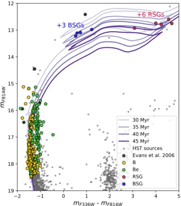
Following Milone et al. (2018) we overplot single-star non-rotating Padova isochrones (Bressan et al. 2012; Chen et al. 2014, 2015; Tang et al. 2014; Marigo et al. 2017; Pastorelli et al. 2019)4_{. We adopt the standard values for the SMC, i.e., the}

dis-tance of d = 60 kpc (Harries et al. 2003; Hilditch et al. 2005; Deb & Singh 2010), the metallicity Z= 0.002 (Brott et al. 2011), the foreground extinction E(B − V) = 0.08 (Keller et al. 1999, D. Lennon, priv. comm.), the SMC extinction law by Gordon et al. (2003), and consider isochrones for ages between 30 and 45 Myr. While we find a good agreement of the isochrones of 35 and 40 Myr with the uppermost part of the main sequence, none of the isochrones reproduces the fainter end of the main se-quence (stars fainter than F814W = 20, not included in Fig. 16 but see Appendix C for a zoomed-out version). They are system-atically too faint by ≈ 0.3 mag.

This effect can also be seen in the CMDs showed in Milone et al. (2018) and Sirianni et al. (2002). While Sirianni et al. (2002) use different HST data and different isochrones from Schaerer et al. (1993), we use the data from Milone et al. (2018) and the same Padova isochrones with slightly different input values (i.e., they adopt d = 57.5 kpc, E(B − V) = 0.11, and a galactic extinction law). Trying to reproduce their findings using the same input values we find that the shape of the isochrones is slightly dif-ferent. This might be due to updates in the codes used to derive the isochrones (several updates were released in 2019, including a new version of the code producing isochrones, Marigo et al. (2017)).

When fitting the isochrone we thus focus on the upper part of the B-star MS which is best reproduced by the isochrones at 35 and 40 Myr. The isochrones at 30 and 45 Myr do not fit the top part of the stars (see also Fig. C.1). This leads to an age estimate of 35 − 40 Myr. We note that the isochrones reproduce the position of the RSGs and BSGs in the CMD very well.

Patrick et al. (subm.) estimate the age of NGC 330 based on the population of RSGs (see also Britavskiy et al. 2019). They find a cluster age of 45 ±5 Myr, which is in good agreement with what is presented here, which is not surprising given the how well the isochrone fitting method reproduces the location of the RSGs in Fig. 16.

We find the cluster turn-off to be at F814W ≈ 16.5 mag which corresponds to M ≈ 7.5 M, which is just below the limiting

mass for neutron star formation. This indicates that all currently produced binary Be stars may remain in the cluster, as their com-panions are likely white dwarfs.

Several stars in the CMD are brighter and hotter than the clus-ter turn-off, i.e. they could be blue stragglers. Half of them are B

4 _{obtained from http://stev.oapd.inaf.it/cgi-bin/cmd}

2 1 0 1 2 3 4 5

m

- m

m

+3 BSGs

+6 RSGs

Fig. 16. Reconstructed CMD from Milone et al. (2018) where their complete input catalog containing field and cluster stars (see their Fig. 2) is shown in grey. The sources with MUSE spectra available are col-ored in terms of the spectral type we derived from the MUSE data, i.e. Be stars in green, B stars in yellow, RSGs in red and BSGs in blue. The eight sources studied by Evans et al. (2006) included in the HST data are indicated with black circles. Overplotted are single-star non-rotating Padova evolutionary tracks for ages between 30 and 45 Myr. Three A-type supergiants and six RSGs are missing in the HST catalog and thus can not be included in this diagram.

stars while the other half are Be stars. These stars are expected to have gained mass in previous binary interactions. They are thus some of the best candidates for BiPs.

5.3. Be stars

Among the 251 B- and O-type stars there are 80 Be stars as well as two Oe stars, indicating a lower limit on the Be star fraction of fBe = 32±3%. This fraction is high compared to typical Be

star fractions of around 20% (Zorec & Briot 1997) measured in field or cluster stars in the Milky Way. The latter fraction is de-termined using several years of observations of bright galactic stars. Due to the variability of Be stars and the disappearance of the emission lines on timescales of months or years (Rivinius et al. 2013), our fraction based on one observational epoch is a lower limit on stars that display the Be phenomenon.

Several previous studies derive high Be star fractions (of the or-der of 50%) in NGC 330 (Feast 1972; Mazzali et al. 1996; Keller & Bessell 1998). They are, however, based on small sample sizes and focus on stars in the outskirts of the cluster. Evans et al. (2006) study a sample of 120 stars in the outskirts of NGC 330 (see Fig. 1) and find a Be fraction of fBe= 23±4 %. Our detected

Be star fraction is significantly higher than the one measured by Evans et al. (2006).

Interestingly, the two earliest-type stars in the sample have Hα, He I, and O I emission while they also show He II absorption.

They are classified as Oe/Be stars (see Sect. 4.3). Using the CMD, we identify them as blue stragglers, i.e. BiP candidates. As shown by the Be star fraction in Fig. 14 the spectral type dis-tribution of Be stars seems to be bimodal, with a shift to later spectral types. As explained in Sect. 4.3, this could be due to the infilling of spectral lines by the emission component, which in particular leads to weaker He I lines and thus a classification into a later spectral type. Additionally, rapidly rotating stars are likely to appear cooler and would subsequently be classified up to two spectral types later than a non-rotating star (Townsend et al. 2004).

In Fig. 17 we instead consider the fraction of Be stars as a function of HST magnitude (F814W) as it is less sensitive to these effects, assuming the population is coeval. It shows that the Be star fraction is between 50 and 75% for stars brighter than 17.0 mag in F814W (corresponding to 7.0 M, according

to Padova isochrones) and rapidly drops below 20% for stars fainter than 17 mag in F814W. This drop corresponds to the cluster turn-off at F814W = 16.5 mag (i.e. M ≈ 7.5 M). We

quantitatively estimate the effect of emission in the Paschen se-ries on F814W photometry from the MUSE spectra. We find that even the strongest Paschen emission series amounts to only ≈ 0.01 mag in the F814W band, and hence is negligible. We furthermore see a similar trend when considering F336W mag-nitudes instead of F814W magmag-nitudes in the histogram. The lack of fainter Be stars could indicate the cut-off luminosity (or mass) for which B-type stars do not appear as Be stars any-more. This could either be due to the fact that these stars do not develop a disk, or to fact that the ionizing flux emitted by these fainter stars is not high enough to ionize the Be star disk (Bastian et al. 2017).

A high-mass X-ray binary ([SG2005] SMC38) is reported within the MUSE FoV (Shtykovskiy & Gilfanov 2005; Sturm et al. 2013; Haberl & Sturm 2016). Giving the crowding of the re-gion and the uncertainty in the position of the source of 0.7" an unambiguous assignment to one of our sample stars is not pos-sible. The two closest stars (i.e. within the errors of the XMM position) are #68 and #80, a B5Ve and a B4V star, respectively. In both cases, and given the position of the system in the cluster core, the massive but hidden companion may be a black hole. In the case of a neutron star, it is likely that the system would have been ejected in the supernova explosion. Given the distance of the SMC, even at low kick velocities of vkick ≤ 2km/s, the

system would have moved 20 pc within 10 Myr, i.e. out of the MUSE FoV. A more in-depth analysis of this object will follow in a subsequent paper of this series.

5.4. Estimate of the total mass of NGC 330

In order to estimate the total mass of NGC 330 we make use of the HST data to determine a scaling factor for the initial mass function (IMF) to the local star density of NGC 330. For this we need an estimate of the total stellar mass in a certain mass bin. Following Milone et al. (2018) we define the cluster core to have a radius of 24" and only consider stars within that distance from the center. As the HST data cover a wider region than the MUSE data we take a less crowded region towards the edge of the HST data in order to estimate the contamination by field stars. From the isochrone fit to the blue main sequence in the CMD (see Fig. 16) we count the number of stars between 3 and 5 M

in the cluster as well as in the field region. We find that there are 412 between 3 and 5 M, which corresponds to a total mass of

1650 Min this mass bin. In comparison, the mass of the field

population in that same mass bin, which we subtract from the

14.5 15.0 15.5 16.0 16.5 17.0 17.5 18.0 18.5

mF814W

Counts

Be star fraction [%]

Fig. 17. Distribution of B and Be stars (in green and yellow, respec-tively) over F814 magnitude taken from Milone et al. (2018) where the left axis shows the total number of stars and the right axis indicates the Be star fraction in each bin. The top axis indicates the conversion from F814W magnitude to mass taken from the Padova isochrones. Stars brighter than F814W = 16.5 are above the cluster turn-off where their mass remains mostly constant while they increase in brightness.

cluster mass, is only 94 M. Comparing this to the integrated

IMF in the same mass bin gives us a scaling factor that scales the IMF to the local star density of NGC 330.

Assuming a Kroupa IMF (Kroupa 2001) and the occurence of stars with masses between 0.01 and 100 Mwe derive a total

mass of the cluster of Mtot,NGC330= 88 × 103M.

In order to estimate an error on the total cluster mass we in-spect the sensitivity of the estimate to the assumptions we made. The total cluster mass increases by 5% if we do not subtract the field population when estimating the mass between 3 and 5 M.

While the mass estimate is not altered significantly by assum-ing a different high-mass end of the IMF, it depends strongly on the low-mass end: Taking a low-mass end of 0.08 M

(in-stead of 0.01 M) the total cluster mass is 4% lower. The

as-sumption that is affecting the estimate the most is, however, the assumed cluster radius. Increasing and decreasing the radius by 25% results in a total mass of Mtot,NGC330 = 105 × 103Mand

Mtot,NGC330 = 70 × 103M, respectively. We thus take this as the

dominating uncertainty which results in a total cluster mass of

Mtot,NGC330 = 88+17₋₁₈× 103M.

Mackey & Gilmore (2002) estimate a mass of 38 × 103_M based

on the surface brightness profile derived from archival HST data. McLaughlin & van der Marel (2005) find a similar value of 36 × 103M. As an order of magnitude estimate, we agree with

their mass estimate within a factor of two. Patrick et al. (subm.) estimate the dynamical mass of NGC 330 based on the veloc-ity dispersion of several RSGs and find a dynamical mass of Mdyn = 158+76−51× 10

3_M

, which is significantly larger than our

estimate. The authors comment that this could be due to the ef-fect of binarity on the determination of Mdyn.

O7 O8 O9 B0 B1 B2 B3 B4 B5 B6 B7 B8 B9

Spectral type

Counts

Fig. 18. Distribution of spectral types from Evans et al. (2006, outskirts) compared to the MUSE data (see Fig. 14) of the core. As there are no stars fainter than V = 17 in the sample of Evans et al. we cut our sample at this brightness to facilitate the comparison.

5.5. Inner regions vs. outskirts

Figure 18 compares the spectral type distribution of Evans et al. (2006) with a subsample of this work adopting the same magni-tude cutoff, i.e. V < 17 mag. This only leaves 22 main-sequence stars in our sample. It can be seen that there are significantly more early-type stars in the sample of Evans et al. (2006). This trend persists when we only include stars from Evans et al. (2006) that are closer than a certain distance from the cluster core, reducing the probability of including field stars. This could be due to a systematic difference in spectral typing, although this is not supported by the two stars that are in common between the two samples (see Sec. 5). It could also indicate that the stars in the sample of Evans et al. are younger and more massive than the core population.

Furthermore we find a significantly higher Be star fraction in the core compared to the outskirts. Restricting our sample to stars brighter than V = 17, which is the brightness limit of Evans et al., we find a Be star fraction of fBe= 46 ± 10 %, while the

frac-tion detected by Evans. et al. is fBe= 23 ± 4 %.

Another significant difference between the core and the outskirts is the different binary fraction. Based on observations spread over only 10 days, Evans et al. (2006) report a particularly low observed binary fraction of only (4 ± 2)%. In this study, based on a single epoch, we find a lower limit on the observed binary fraction of (14 ± 2)%, which is higher than the fraction derived by Evans et al. (2006).

These findings combined reveal that the stellar content of the core and the outskirts are clearly different, with the stars in the outskirts significantly younger. We note this is the opposite of what was found in 30 Doradus, where the core cluster (R136) is significantly younger than the average age of the massive stars in NGC 2070 and the wider region (Crowther et al. 2016; Schnei-der et al. 2018).

The two distinct populations seen in/around NGC 330 could be explained by different star-formation histories, with the older cluster contrasting with younger stars formed as part of the on-going (more continuous) star formation in the SMC bar. Indeed, given the 35-40 Myr age of the cluster, feedback from when the

most massive stars in the cluster exploded as supernovae could have helped instigate star formation in the outskirts.

Alternatively, rejuvenated runaway or walkway stars (see e.g., Renzo et al. 2019) could contribute to the younger population in the outskirts. These stars would be the mass gainers in pre-vious binary interactions (thus appearing rejuvenated) that had been ejected when their previously more massive companions exploded as supernoave. Assuming a low ejection velocity of 5 km/s a star would travel 50 pc within 10 Myr which indicates that the population of the outskirts (i.e. outside the MUSE FoV) by runaway or walkaway stars is possible.

More detailed study is required to understand the formation his-tory of these populations, supported by detailed physical param-eters of the stars and combined with dynamical information from their radial velocities and proper motions.

6. Summary and future work

This is a first study of the dense core of the SMC cluster NGC 330 using the MUSE-WFM equipped with the new AO. Using the unprecedented spatial resolution of MUSE WFM-AO allows us to spectroscopically study the massive star population in the dense core of the cluster for the first time. We automati-cally extract and normalize spectra for more than 250 stars. We find that a vast majority of them are B-type stars while there are also two Oe stars and a handful of RSGs and BSGs. Around 30% of the B stars (and both O stars) show broad spectral lines char-acteristic of rapid rotation and emission features primarily in Hα but also in other spectral lines like He I and O I. They are thus classified as classical Be (Oe) stars. We derive a lower limit on the observed binary fraction of 14 ± 2%.

Using archival HST data we are able to position our stars in a color-magnitude diagram and investigate their evolutionary sta-tus. Comparing to single-star non-rotating Padova isochrones we estimate a cluster age between 35 and 40 Myr and a total cluster mass of Mtot,NGC330= 88+17₋₁₈× 103M. This mass can be used to

compare our findings for NGC 330 to clusters of similar masses but different ages, for example RSGC 01, RSGC 02, RSGC 03, or NGC 6611 in the Milky Way, and NGC 1818, NGC 1847 or NGC 2100 in the LMC (Portegies Zwart et al. 2010).

We find several stars that are hotter and brighter than the main-sequence turn-off, indicative of blue straggler stars which are thought to be binary-interaction products. Two of these stars, classified as Oe/Be stars are the stars of earliest spectral type in our sample and could have been spun up to high rotational velocities in previous binary interactions.

Comparing our findings to the spectroscopic study of 120 OB stars in the outskirts of NGC 330 by Evans et al. (2006) we find significant differences in the spectral type distribution, the Be star fraction and the binary fraction. We conclude that the stellar content of the core is significantly different from the one in the outskirts and discuss possible explanations.

In subsequent papers of this series we will determine the cur-rent multiplicity fraction of all stars in the sample using the 6 epochs we have available. This will also allow us to characterize the variability of the Be stars in the sample. Subsequently, we will combine all 6 epochs to increase the S/N of the data which will allow us to model the stars in order to derive their effective temperatures, surface gravities, rotation rates, and abundances for the brightest stars. This will allow us to further investigate the BiP candidates identified in this paper and characterize the star formation history of NGC 330.

Acknowledgements. J.B. acknowledges support from the FWO_Odysseus pro-gram under project G0F8H6N. L. R. P acknowledges support from grant