Deterministic chaos in models of human behavior : methodological issues and experimental results

HD28 .M414

Ki'i^-B}

^<^%. »«s,,

TsS;;--NOV

12

1987 «Pr

WORKING

PAPER

ALFRED

P.

SLOAN SCHOOL

OF

MANAGEMENT

DETERMINISTIC CHAOS

IN

MODELS

OF

HUMAN BEHAVIOR:

METHODOLOGICAL ISSUES AND EXPERIMENTAL RESULTS

JOHN

D.

STERMAN

OCTOBER

1987

_{WP 1945-87}

MASSACHUSETTS

INSTITUTE

OF

TECHNOLOGY

50

MEMORIAL

DRIVE

CAMBRIDGE,

MASSACHUSETTS

02139

r

'^

DETERMINISTIC CHAOS

IN

MODELS

OF

HUMAN BEHAVIOR:

METHODOLOGICAL ISSUES AND EXPERIMENTAL RESULTS

JOHN

D.

STERMAN

D-3921

Deterministic

Chaos

in

Models

of

Human

Behavior:

Methodological

Issues

and

Experimental

Results

John D.

Sterman

Associate Professor Sloan School of

Management

Massachusetts Institute of

Technology

Cambridge,

MA

02139

Forthcoming

in the

Special Issue

on

Instabilities

and

Chaos

System

Dynamics

Review

D-3921

ABSTRACT

Recent

work

has

shown

that several

well-known models

in the system

dynamics

literature contain previously unsuspected regimes ofdeterministic chaos.

Two

of the

most

extensively analyzed are Sterman's

model

of the

economic

long

wave

and

the

production-distribution

model

of the

Beer

Distribution

Game.

The

significance of these theoretical

developments hinges

on

whether the chaotic regimes lie in the realistic region of parameter

space. Further there are

major

questions regarding the descriptive accuracy of

models

of

human

systems

which

exhibit chaos. Data limitations and the inability to conduct controlled

experiments

mean

empirical studies at the aggregate level are not likely to resolve these

questions.

An

alternative approach is based

on

laboratory experiments in

which models

provide a simulated environmentfor the study of

human

decisionmaking behavior. Recently

laboratory experiments have been conducted to analyze decisionmaking behavior in the long

wave

model

and the

Beer

Distribution

Game.

This paper describes the experiments and

shows

that the behavior ofthe subjects is explained well with a simple heuristic long used in

system

dynamics modeling

and well

grounded

in behavioral decision theory.

The

parameters ofthe proposed decision rule are estimated econometrically for each subject.

The

parameters

which

characterize a significant minority of the subjects are

shown

to produce chaos. This

direct experimental evidence thatchaos can be

produced by

the decisionmaking behavior of

realpeople has important implications for the formulation, analysis,

and

testing of

models

of

D-3921

Recent

work

has

shown

that several

well-known models

in the system

dynamics

literature contain previously unsuspected regimes of deterministic chaos.

The

work

of

Day

(1982a, 1982b) provides an early

example

of chaotic behavior in

economic

models, while

Mosekilde

and others (1987) have developed corporate

models which

exhibit chaos.

Two

of

the

most

extensively analyzed such

models

are Sterman's

model

ofthe

economic

long

wave

(Sterman 1985, 1986,

Rasmussen,

Mosekilde,

and Sterman

1985) and the

production-distribution system or

Beer

Distribution

Game

(Forrester 1961, Jarmain 1963,

Sterman

1984,

Mosekilde and

Larsen, this issue).

While

the demonstration that chaos can be

endogenously

produced

in these systems is an important theoretical development, the significance of the

results hinges in large

measure

on whether the chaotic regimes lie in the realistic region of

parameter space or

whether

they are mathematical curiosities never observed in the real

system. Further there are

major

questions regarding the descriptive accuracy of the decision

rules postulated in the

models

of

human

systems developed to date

which

contain strange

attractors.

The

practical significance of chaos

and

other

phenomena

such as self-organization

in policy-oriented

modeling

remains unclear until it can be determined that these

phenomena

can occur in

models

whose

decision rules are

grounded

in empirical study ofthe actual

decision processes of the agents. It is difficult if not impossible to resolve such issues

by

appeal to the aggregate empirical data. In the case of the long wave, for example, there

have

been at

most

five

long-wave

cycles since the industrial revolution, too

few

for statistically

reliable results.

Worse,

the data required are simply unavailable, and

much

ofit is corrupted

by

measurement

error (Chen, this issue).

An

alternative approach is based

on

laboratory experiments in

which models

provide a

simulated

environment

for the study of

human

decisionmaking (Sterman 1987a). Recently,

the long

wave

model and Beer

Distribution

Game

(traditionally used as a teaching rather

(Sterman 1987b, 1987c).

These

experiments

were

conducted primarily to study the heuristics

with

which

people

manage

a

complex dynamic

environment. In both experiments the decision

task ofthe subject

was

to

manage

a stock in the face oflosses, delays in acquiring

new

units,

multiple feedbacks

and

other environmental disturbances.

This paper describes the experiments

and

shows

that decisionmaking behavior in the

two

experiments is significantly suboptimal.

The

departures

from

optimal behavior are

systematic, suggesting subjects use

common

heuristics for stock

managment.

The

experiments

show

that the behavior of the subjects can be

modeled

well with a simple

stock-management

heuristic long used in system

dynamics modeling and

well

grounded

in

behavioral decision theory.

The

parameters of the proposed heuristic are estimated

econometrically for each subject.

The

systems are then simulated with the estimated parameters.

The

parameters

which

characterize a significant minority of the subjects are

shown

to produce chaos. This direct experimental evidence thatchaos can be

produced by

the decisionmaking behavior ofreal people has important implications for the formulation,

analysis, and testing of

models

of

human

behavior.

The

Stock

Management

Problem

The

regulation ofa stock or system state is one of the

most

common

dynamic

decisionmaking tasks.

The

manager

seeks to maintain a quantity at a target level, or at least

within an acceptable range. Stocks cannot be controlled directly but rather are influenced by

altering the stock's inflow

and

outflow rates. Typically a

manager must

set the inflow rate so

as to

compensate

for losses

from

the stock and to counteract environmental disturbances

which

may

push

the stock

away

from

its desired value. Frequently there are lags

between

the initiation ofa control action and its effect

on

the stock, and/or lags

between

a change in

the stock and the perception ofthat change

by

the decisionmaker.

The

duration of these lags

may

vary and

may

be influenced by the manager's

own

actions.

D-3921

Stock

management

problems occur at

many

levels ofaggregation

from

the micro to the

macro.

At

the level ofa firm,

managers

must

order parts

and

raw

materials so as to maintain

inventories sufficient for production to proceed at the desired rate, yet prevent costly

inventories

from

piling up.

They must

adjust for variations in the usage and wastage of these

materials

and

for changes in theirdelivery delays.

At

the level ofthe individual, people

regulate the temperature ofthe water in their

morning

shower, guide their cars

down

the

highway, and

manage

their checking account balances.

At

the

macroeconomic

level, the

Federal Reserve seeks to

manage

the stock of

money

so as to provide sufficient credit for

economic growth

while avoiding inflation and compensating for variations in credit

demand.

The

generic stock

management

control

problem

may

be divided into

two

parts: (i) the

stock and flow structure ofthe system;

and

(ii) the decision rule used

by

the

manager

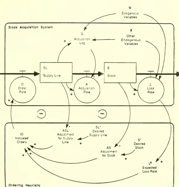
(figure

1). Considering first the stock and flow structure, the stock of interest S is the accumulation

ofthe acquisition rate

A

less the loss rate L:

Si=

I

(A,-L^)dx+S,

' '

K

^ (1)

Losses

from

the stock

must depend on

the stock itself,

and

may

also

depend on

other

endogenous

variables

X

and

exogenous

variables U:

Lt

=

fL(St,Xt,Ut). ₍₂₎

The

acquisition rate will

depend on

the supply line

SL

ofunits

which

have been ordered but

not yet received, and the average acquisition lag X. In general,

X may

be a function of the

supply line itself

and

the other

endogenous

and

exogenous

variables:

At

=

fA(SLat).

(3)

The

supply line is simply the accumulation ofthe orders

which have

been placed

O

less those

which have

been delivered:

SL,=

I

(O,-

A,)dx+SL,

The

structure represented by figure 1 and eq. (1-4) is quite general. There is

no

presumption

that the functions governing losses

and

the acquisition lag are linear. There

may

be

arbitrarily

complex

feedbacks

among

the

endogenous

variables,

and

the system

may

be

influenced by

numerous exogenous

forces including noise and nonstationarity ofthe

underlyingequilibrium.

Consistent with the behavioral foundations of system

dynamics modeling

(Morecroft

1983, 1985,

Sterman

1987a), behavioral decision theory (Hogarth 1987,

Tversky

and

Kahneman

1974), and the theory of

bounded

rationality

(Simon

1979, Cyert and

March

1963),

the proposed decision rule utilizes information locally available to the decisionmaker and does

not

presume

the

manager

has global

knowledge

of the structure of the system.

The

generic

decision rule recognizes three motives for ordering

which

any stock

management

heuristic

must

include:

Order

enough

to (1) replace expected losses

from

the stock, (2) reduce the

discrepancy

between

the desired

and

actual stock,

and

(3) maintain an adequate

.supply line ofunfilled orders.

1.

Replacement

_oflosses.

The

replacement motive is straightforward. In equilibrium,

when

the desired

and

actual stock are equal, the

manager must

continue to order

enough

to

replace

ongoing

losses. Losses

may

arise

from

usage (e.g. shipments

from

an inventory of

finished goods) or decay (e.g. the depreciation of plant

and

equipment). Failure to replace

losses

would

cause the stock to fall

below

the desired level, creating steady-state error.

2. Stock adjustment. Errors in forecasting losses or changes in the desired stock

demand

a

mechanism

to adjust orders

above

or

below

replacement. Orders to reduce the

discrepancy

between

thedesired and actual stock

form

a negative feedback loop

which

regulates the stock

(shown

in the

bottom

part of figure 1).

Any

rule

which

fails to

compensate

for discrepancies

between

the desired and actual stock fails to control the stock

D-3921

the desired value ifdisplaced.

The

stock

would

follow a

random

walk

as the system is

bombarded

by shocks.

3. Supply line adjustment. Delays

between

the initiation and impact ofcontrol actions

give stock

management

systems significant inertia

and

should be accounted for

by managers

to ensure a stable response to shocks. Failure to account for the supply line results in

overcorrection and instability. Consider cooking dinner on an electric range. Ifone turns the

heat

down

just as thepot

comes

to a boil the supply line ofheat in the coils of the range will

continue to heatthe pot, boiling it overand ruining dinner.

The

following equations formalize the ordering heuristic

proposed

above. First, orders

in

most

real life situations

must

be nonnegative,

Ot

=

MAX(0,IOt)

₍₅₎

where

10

is the indicated order rate, the rate indicated by other pressures. ^

The

indicated order rate is based

on

the anchoring

and

adjustment heuristic (Tversky

and

Kahneman

1974).

Anchoring and

adjustmentis a

common

judgmental strategy in

which

an

unknown

quantity is estimated by first recalling a

known

reference point (the anchor)

and

then adjusting for the effects of other factors

which

may

be less salient or

whose

effects are

obscure.

Anchoring and

adjustment has been

shown

to apply to a

wide

variety of

decisionmaking tasks

(Einhom

and Hogarth

1985, Davis,

Hoch,

and Ragsdale 1986,

Johnson

and

Schkade

1987,

Lopes

1981, Hines 1987,

Sterman 1987dX

Here

the anchor is the

expected loss rate L^. Adjustments are then

made

in response to discrepancies

between

the

desired and actual stock

AS

and

between

the desired and actual supply line

ASL:

lOt = L^t +

ASt

+ ASLt. (6)

The

expected loss rate

may

be

formed

in various ways.

Common

assumptions in

equilibrium value), regressive expectations L^t= yLt-l + (l-Y)L*, 0<y<l, adaptive

expectations

L«t=

6Lt-i

+

(l-6)L^t-l,

0<9<1, and

extrapolative expectations, AL^t =

lcoi*ALt-i,

where

A

is the first-difference operator

and

coi>0.

The

adjustment for the stock

AS

creates the chiefnegative feedback loop

which

regulates the stock.

The

proposed

heuristic

assumes

for simplicity that the adjustment is

linear in the discrepancy

between

the desired stock

S*

and the actual stock:

ASt

=

as(S*t-St)

(7)

where

the stock adjustment parameter

as

is the fraction ofthe discrepancy ordered each

period.

The

adjustment for the supply line is formulated analogously as

ASLt

=

asL(SL*t-

SLt) (8)

where

SL*

is the desired supply line

and asL

is the fractional adjustment rate for the supply

line.

The

desired supply line in general isnot constant but

depends

on

the desired throughput

O*

and the expected lag

between

ordering and acquisition of goods:

SL*t =

Xh*0*t.

(9)

The

adjustment for the supply line creates a second negative feedback loop

which

avoids overordering

and

also

compensates

for changes in the acquisition lag X. If

X

rises, for

example,

ASL

induces sufficient additional orders to restore

A=0*.

There

are a varier>' of

possible representations for X^ and

O*,

ranging

from

constants through sophisticated

forecasts.

Experiment

I:

The

Economic

Long

Wave

The

experimental protocol for the long

wave

model

is described in

Sterman

and

Meadows

1985 and

Sterman

1987a, 1987b).

The

methodological foundations of experimental

economics

are discussed in the seminal

work

of Smith (1982) and Plott (1986).

The model

D-3921

hypothesis behind the long

wave

can be stated in

two

parts. First,

due

to construction lags,

the process by

which

individual firms adjust production capacity to

demand

is inherently

oscillatory. In isolation an individual firm

would

produce

damped

fluctuations with aperiod of

about 15-25 years in response to a shock. Second, in the aggregate the capital-producing

sector of the

economy

orders and acquires capital

from

itself. This multiplier effect or

'self-ordering' creates a positive feedback loop

which

destabilizes the oscillatory tendencies of

individual firms, changing the

damped

oscillation to a limit cycle with a

40-60

yearperiod.

Simulation

and

formal analysis confirm the

dynamic

hypothesis (Sterman 1985;

Rasmussen,

Mosekilde

and

Sterman

1985).

As

the self-ordering loop

becomes

stronger,

damping

drops

rapidly.

The

system goes through a

Hopf

bifurcation and produces a limit cycle. Further

increases in the strength of self-ordering proceed through period doublings and ultimately to

chaos.

In the experiment the

model

is transformed into a

game

in

which

subjects

manage

the

capital-producing sector of a simple

economy.

Subjects

must

balance the supply of

and

demand

for capital

by

adjusting their production capacity to

meet

desired production. Orders

for capital arise

from

the

exogenous

consumer goods

sector and

from

the subject's

own

orders.

The

equations underlying the

game

reflect a simplified

form

ofthe original

model

but

preserve its essential structure

and

dynamics. In the

game

decisions are

made

in discrete

time intervals representing

two

years, and the

model

becomes

a third-order difference

equation system.

The

equations ofthe

game

are given below. Production

PR

is the lesser ofdesired

production

DP

orProduction Capacity PC. Capacity is proportional to the capital stock.

The

capital/output ratio

k

is

one

period (two years):

PRt

=

MIN(DPt,PCt)

(10)

The

capital stock ofthe capital sector is

augmented by

acquisitions

AK

and diminished by

depreciation

CD.

Depreciation is proportional to the stock.

The

average lifetime ofthe

capital stock x is 10 periods (20 years):

Kt+i

= Kt + (AKt-CDt)

(12)

CDt

=

Kt/t. (13)

The

acquisition ofcapital by both the capital and

goods

sectors

(AK

and

AG)

depends

on

the

supply line ofunfilled orders each has accumulated (the backlogs

BK

and

BG)

and

the fraction

of

demand

satisfied

FDS.

Each

period both the capital

and goods

sectors acquire the full

supply line of unfilled orders unless the capital sector is unable to produce the required

amount. In this case acquisition

by

each sector is reduced in proportion to the shortfall.

The

acquisition lag

X

is thus 1/FDS,

and

AK+AG=PR

at all times, ensuring that output is

conserved:

AKt

=

BKt*FDSt

(14)

AGt

=

BGt*FDSt

(15)

FDSt

= PRt/DPt

(16)

DPt

=

BGt

+

BKt. (17)

The

supply lines of unfilled orders foreach sector

BG

and

BK

are

augmented

by orders for

capital placed by each sector

and

emptied

when

those orders are delivered:

BKt+i

=

_BKt

+

(OKt

-

AKt)

(18)

BGt+i

=

BGt

+ (OGt-AGt).

(19)

New

orders placed

by

the

goods

sector are the

exogenous

input to the system to

which

the

subject ofthe experiment

must

respond

by

choosing an appropriate

amount

ofcapital to order

for their

own

use:

OGi

= exogenous

(20)

OKt

=

determined

by

subject. (21)

D-3921

9

of the subjects in

making

these decisions is to minimize their total score for the trial.

The

score is defined as the average absolute deviation

between

desired production

DP

and production capacity

PC

over the

T

periods of the experiment:

T

S

=

(1/T)

S

I

DPt

-

PCt

|. (22)

t=0

The

score indicates

how

well subjects balance

demand

and supply. Subjects are penalized equally for both excess

demand

and

excess supply.

The

experiment is

implemented on

IBM

PC-type

microcomputers.

A

'gameboard' is

displayed

on

the screen providing subjects with perfect information. Color graphics and

animation highlight the flows oforders, production, and shipments to increase the

transparency ofthe structure.

The

conversion ofthe original

model

to a

form

suitable for

experimental testing is described in

Sterman

1987a.

The

subject population

(N=49)

consisted of

MIT

undergraduate, master's and doctoral students in

management

and

engineering,

many

with extensive exposure to

economics

and

contro^ theory; scientists and economists

from

various institutions in the

US,

Europe, and the

Soviet Union; and business executives experienced in capital investment decisions including

several

company

presidents and

CEOs.

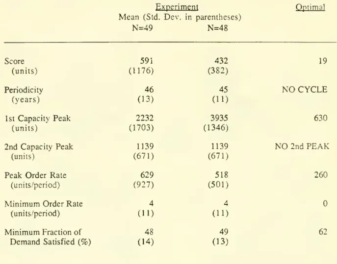
Typical experimental results are

shown

in figure 3. All trials begin in equilibrium. In

period 3 there is a one-time step inputof

10%

in the orders ofthe

goods

sector.

The

optimal

responsereturns the system toequilibrium within 6 periods, producing a score of 19. In

contrast the vast majority ofsubjects

produced

significant oscillations (table 1).

The

average

score for the

sample

was

591; the lowest

was

77.

Next

the

proposed

stock

management

heuristic (equations 5-9)

was

tested against

the ordering behavior of the subjects. Adapting the heuristic to the experimental context is

proportional to desired production.

The

loss rate

L

is simply the depreciation ofthe capital

stock

CD. The

desired supply line

DSL

was

specified according to equation 9, with the

expected acquisition lag X^

=X=

1/FDS

and desired throughput

0*=

CD.

Allowing

an

additive disturbance term E, the proposed ordering rule for capital investment

becomes:

OKt

=

MAX(0,CDt

+

ASt +

ASLt

+ Et) (23)

ASt

=

as(DKt-Kt)

(24)

ASLt

=

asUDSLt

-

BGt)

₍₂₅₎

DSLt

=

?.e*CDt=

(l/FDSt)*CDt.

'

(26)

To

test the rule only the

two

adjustment parameters

as

and

asL

need

be estimated. All other

data required to determine orders are presented directly to the subjects.

Maximum

likelihood estimates of the parameters for each trial

were

found by grid search of the parameter space,

subject to the constraints as,

asL

^0.

Assuming

the errors £ are independent, identical, and

normally distributed then the

maximum

likelihood estimates of such nonlinear functions are

given

by

the parameters

which minimize

the

sum

of squared errors.

Such

estimates are

consistent

and

asymptotically efficient, and the usual measures of significance such as the

t-test are asymptotically valid.

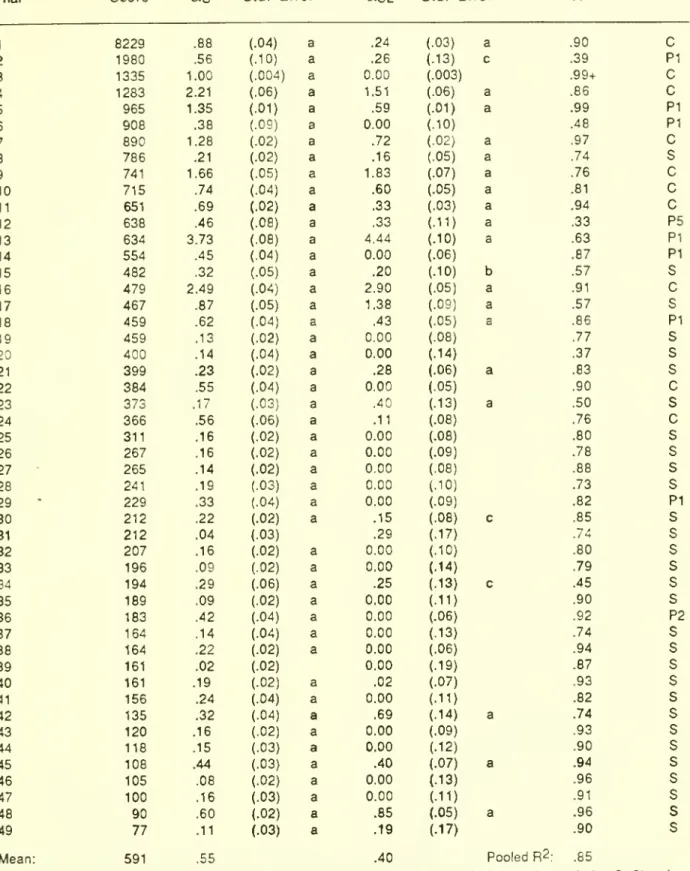
Estimates for

49

trials together with t-statistics are given in table 2.

The

model's

ability to explain the ordering decisions ofthe subjects is excellent.

R2

varies

between

33%

and

99+%,

with an overall

R^

for the pooled

sample

of

85%.2

All but

two

ofthe estimated

capital stock adjustment parameters are highly significant.

The

supply line adjustment

parameter is significant in 22 trials.

Sterman 1987b

analyzes the estimation results and identifies several 'misperceptions

of feedback'

which

are responsible for the subjects'poor performance.

One

ofthese is the

D-3921

11

continue ordering even after the construction pipeline contains sufficient units to correct any

stock discrepancy.

The

present concern, however, is the relationship

between

the estimated

parameters and the regimes of behavior in the model.

The

estimated parameters characterize

the decision

making

behavior of actual people.

When

simulated in the

model

are the

estimated decisoin rules ofthe subjects inherently stable, or

do

they

produce

limit cycles,

period multiples, or chaos?

Table 2 also indicates the

mode

of behavior produced by simulation ofthe decision rule

with the estimated parameters.

The

parameters estimated for thirty subjects

(61%)

are

stable.

Most

of these produce

overdamped

behavior of the capital stock in response to the

step input.

Seven

parameter sets produce limit cycles of period 1, and 2 produce period

multiples.

The

parameters

which

characterize ten subjects

(20%)

produce chaos. Inspection

of table 2

shows

that the subjects

whose

parameters are stable

performed

best in the task

while those

whose

parameters produce limit cycles and chaos generally

had

the highest scores.

Figure 4

shows

the phase portrait for several of the

more

interesting parameter sets.

Note

the period 5 cycle

produced

by (as, asL)

=

(.46, .33).

The

apparent period 2 cycle

produced

by (.42, 0) is,

upon

closer inspection, seen tobe chaotic.

Figure 5 locates the

modes

of behavior in parameter space. Consistent with both

intuition

and

formal stability analysis, stability is

enhanced

by small values of

as

and large

values of asL.

More

aggressive attempts to correct the discrepancy

between

the desired and

actual capital stock are destabilizing: by ordering

more

aggressively the self-ordering loop

causes a larger increase in total

demand,

thus exacerbating disequilibrium and encouraging

still larger orders in future periods. Conversely,

more

aggressive response to the supply line

Thus

the periodic and chaotic attractors tend to occur for large values of

as

and small

values ofasL- Yet the route to chaos is apparently

more

complex. Consider the route to

chaos as

as

increases for asL=0. Stability gives

way

to period

one

limit cycles, then to period

2 at (.42, 0), and ultimately to chaos for

as

^.55.

Yet

the parameters

which

produce the

slightly chaotic period 2 are surrounded

on

the ray

asL

=

by parameters

which

produce

period 1 limitcycles. Similarly, the period 5 attractor

produced

by the parameters (.46, .33)

lies

between

the region ofstability and the region ofperiod 1 behavior.

The

results

show

that the parameters

which

characterize actual decisionmaking

performance in a

common

and important

macroeconomic

situation canproduce a

wide

range of behavior, including chaos.

Experiment

II:

The

Production-Distribution

System

The

"Beer Distribution

Game"

is a role-playing simulation ofan industrial production

and

distribution system developed at

MIT

to introduce students of

management

to the

concepts of

economic dynamics and computer

simulation. In use forneariy three decades, the

game

has been played all over the worid by thousands of people ranging

from

high school

studentsto chief executive officers

and government

officials.

The

game

is played

on

a board

which

portrays in a simplified fashion the production

and

distribution of beer (figure 6). Orders for and cases of beer are represented

by

markers

and

pennies

which

are physically manipulated

by

the players as the

game

proceeds.

Each

brewery

consists of four sectors: retailer, wholesaler, distributor,

and

factory (R,

W,

D, F).

One

person

manages

each sector.

Customer

demand

is represented

on

a

deck

of cards.

Customers

demand

beer

from

the retailer,

who

ships the beer requested out of inventory.

The

retailer in turn orders beer

from

the wholesaler,

who

ships the beer requested out ofthe

D-3921

13

distributor,

who

in turn orders and receives beer

from

the factor^'.

The

factory produces the

beer.

At

each stage there are shipping delays and order receiving delays.

These

represent

the time required to receive, process, ship, and deliver orders, and as will be seen play a

crucial role in the dynamics.

The

subjects' objective is to

minimize

cumulative

team

costs over the length ofthe

game.

Inventory holding costs for each sector are $.50 per case per

week,

and stockout costs

(costs for having a backlog of unfilled orders) are $1.00 per case perweek.

The

decision task of each subject is a clear

example

ofthe stock

management

problem. Subjects

must keep

their inventory as

low

as possible while avoiding backlogs and

satisfying customer

demand.

Inventory cannot be controlled directly but

must

be ordered.

The

lag in receiving beer is potentially variable: ifthe wholesaler has beer sufficient to cover

the retailer's orders the retailer will receive the beer desired afterthree weeks.

But

if the

wholesaler has run out, the retailer

must

wait until the wholesaler can receive additional beer

from

the distributor.

Only

the factory, theprimary producer, faces a constant delay in

acquiring inventory (there is

no

limit to the production capacity ofthe factory).

The

protocol forthe experiment is described in

Sterman

1987c.

The

game

is initialized

in equilibrium.

Each

inventory contains 12 cases.

Customer

demand

is initially four cases per

week.

To

disturb the system customer

demand

increases to eight cases per

week

in

week

5

and

remains at that level thereafter.

The

results reported here

were

drawn from

four

dozen

games

(192 subjects) collected

over a period offouryears.

A

computer model

ofthe

game

was

used to test the records for

consistency. Trials in

which

there

were

accounting errors of

more

than a

few

cases per

week

for

more

than a

few weeks

in any of the four sectors

were

discarded

from

further analysis.

Eleven

games

were

retained, providing

44

subjects.^

That sample

consists ofundergraduate,

MBA,

and

Ph.D. students at

MIT's

Sloan School of

Management,

executives

from

a variety of

firms participating in short courses on

computer

simulation,

and

senior executives of a

major

computer

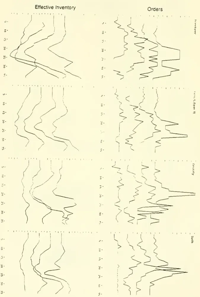
firm.

Typical experimental results are

shown

in figure 7

and summarized

in table 3.

The

results

show

the behavior of the subjects to be far

from

optimal.

The

average

team

cost is

ten times greater than optimal. Like the

macroeconomic

experiment, the results exhibit

several strong regularities.

1. Oscillation:

The

trials are allcharacterized

by

instability and oscillation.

The

pattern oforders and ofinventory is

dominated

by a large amplitudefluctuation with an

average period of 21 weeks.

2. Amplification:

The

amplitude and variance of orders increases steadily as one

moves

from

customerto retailer to factory.

The

peak

order rate at the factory level is

on

average

more

than double the

peak

order rate generated at the retail level.

Customer

orders increase

from

4 to 8 cases perweek.

By

the time the disturbance has propagated to the

factor)', the order rate averages a

peak

of32 cases.

3.

Phase

lag:

The

peak

order rate tends to occur later as

one

moves

from

the retailer

to the factory.

The

phase lag is not surprising since the disturbance in customer orders

must

propagate through decisionmaking and order delays

from

retailer to wholesaler and so on.

Next

the proposed decision rule

must

be adapted to the particular situation in the beer

game

and

cast in a

form

suitable for estimation ofthe parameters.

The

stock

S

corresponds

to the inventory of the subject

and

the supply line

SL

to the

sum

of orders in the mail delays,

the backlog ofthe subject's supplier (ifany), and the beer in the shipping delays.

The

loss

rate is the rate at

which

each subject receives orders.

To

test the rule it is necessary to

specify expected losses L^, the desired stock S*, and the desired supply line SL*.

Expected

losses

from

the stock are the rate at

which

each subject expects their

D-3921

15

the factory's forecast of the distributor's order rate, etc. Adaptive expectations are

postulated. Adaptive expectations are widely used in simulation

modeling

of corporate

and

economic

systems, they are often a

good model

of the evolution of expectations in the

aggregate (Sterman 1987d, Frankel

and

Froot 1987),

and

they are

one

of the simplest

formulations for expectations flexible

enough

to adapt to a nonstationary process.

Because

the subjects lack the information and time to determine optimal inventory orsupply line levels

the desired stock

S* and

desired supply line

SL*

are both

assumed

to be constants

which

must

be estimated.

The

generic decision rule ofeq. (5-9) thus becomes:

Ot

=

MAX(0,IOt)

(27)

IOt=Let

+ ASt +

ASLt

(28)

Let

=

eLt-l + (l-e)Lei.i.

0<e<l

₍₂₉₎

ASt

=

as(S*

- _{St) (30)}

ASLt

=

asL(SL*

- _{SLt). (31)}

Defining P

=

asUct-s and S'

= S* +

PSL*

yields

lOt

=Let

+

as(S'-St-pSLt).

(32)

Note

that since S*, SL*,

asL

and

as

are all >0, S'>0. Further, it is unlikely that subjects will

place

more

emphasis

on

the supply line than

on

the inventor)' itself: the supply line does not

directly enter the cost function nor is it as salient as inventory. Therefore it is probable that

asLS

as,

meaning

0<(3<1.

Thus

(3 can be interpreted as the fraction of the supply line taken

into account

by

the subjects. If

_{P =}

1, then the subjects fully recognize the supply line and

do

notdouble order. If _P

=

0, then orders placed are forgotten until they arrive, encouraging

overordering

and

instabilitj.'^

implemented

in the beer

game

contains four parameters to be estimated (6, as, S', and p).

The

parameters

were

estimated by the

same

procedure used in the long

wave

experiment.

An

additive disturbance term is assumed, and the disturbances are

assumed

to be i.i.d.

normal. Estimates for each sectorofeach trial

were

found

by

grid search of the parameter

space subject to the constraints

0<6<1

and

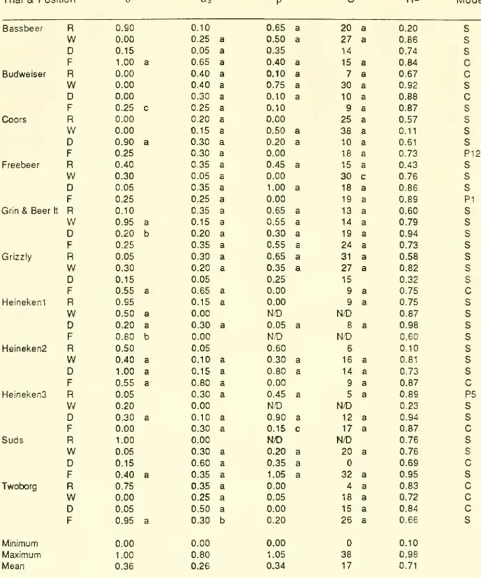
as, S', _p >0.5

The

estimated parameters are displayed in table 4.

The

mean

R2

is

71%;

R^

is less

than

50%

foronly 6 of

44

subjects.^

A

large majority of the estimated parameters are

significant.

As

in thelong

wave

experiment the decision rule is an excellent

model

of the

decisionmaking behavior ofthe subjects.

Sterman

1987c relates the estimated parameters to

the dysfunctional performance in the task. It is noteworthy that the

same

misperceptions of

feedback structure

which

cause oscillation in the

macroeconomic

experiment are responsible

for thepoorperformance ofthe subjects in the beergame. Specifically, the supply line of

unfilled orders is given far too little weight by

most

subjects.

Next

the beer

game

was

simulated using the stock adjustment rule with the

estimated parameters.

Each

trial involves four subjects, each of

whom

could have different

parameters. In the simulations, however, the

same

parameters

were

assumed

for each

sector, vastly simplifying the analysis.*^

Table 4 indicates the

mode

of behavior

produced by

each set ofparameters.

Thirty-one parameter sets

(70%)

produce stable behavior.

One

each produces limit cycles ofperiod

1, period 5, and period 12.

Ten

yield chaos. Since the beer

game

is a 19th order system the

behavior

produced

by the system is exceedingly

complex

and there are

many

possible

projections of phase space. Figure 8

shows

several of the

more

interesting phase portraits.

D-3921

17

parameters of the Bassbeer Factory (9, as, P, S' = 1, .65, .40, 15)

compared

to those of the

HeinekenS

Factory (9, as, P, S'

=

0, .3, .15, 17).

The

parameters estimated for the

Coors

Factory (9, as, p, S' = .25, .3, 0, 18) reveal a cycle ofperiod 12

when

distributorinventory is

plotted against factory inventory.

The

retail sector ofthe

same

team, however, produces a

limit cycleofperiod 1.

The

difference in

mode

is probably due to the integer constraint

on

orders.

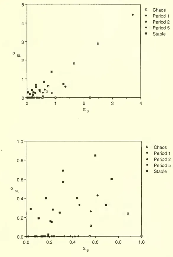
Figure 9

shows

the distribution ofthe

modes

in parameter space.

The

relationships

between

the adjustment parameters

and

stability are similar to those apparent in the

macroeconomic

experiment,

and

for similar reasons. In general, larger values of

as

and

smaller values _{of P} are destabilizing. That is, to the extent the subjects ignore the supply

line of unfilled orders (P=0) a stock discrepancy will cause orders to be placed each period

even after sufficient orders are in the supply line, leading to excess inventories and

oscillation.

Such

overordering is exacerbated by

more

aggressive stock adjustment

(as>>0)

since

more

will be ordered in response to a given discrepancy

between

the desired

and

actual

stock. Figure 9 also indicates that in general the smaller the desired inventory S' the less

stable the system. Again, intuition readily explains

why

this is so. Consider the response of

the retailer to an unanticipated increase in customer

demand.

Retail inventory falls

due

to the

lags in receiving beer.

The

retailer will place additional orders with the wholesaler through

the stock adjustment term. Ifthe wholesaler has adequate inventory to fill

incoming

orders

(S'»0)

incoming

orders can all be filled and the retailer's acquisition lag remains constant.

If, however, the wholesaler runs out ofinventory the retailer finds orders placed fail to arrive.

The

delay in receiving beer lengthens, the retailer's stock drops still further,

and

still

more

orders swell the supply line in a vain attempt to replenish inventory.

When

sufficient beer

(figure 7). S' plays such a crucial role in determining the stability of the system because it

determines

how

close the system operates to the fundamental nonlinear contraint that

shipments can only be

made

if inventor)' exists. Small values ofS'

make

it

more

likely the

system will run out ofinventory thus entering the unstableregion in

which

the acquisition lag

X

is long

and

variable.

Those

subjects

who

maintained larger target inventory levels

were

thus

more

stable

on

average than those

who

attempted to cut costs

by

reducing their buffer

stock.

There

appears to be

no

simple relationship

between

the parameter 6

and

the

modes

of

the system. 6 controls the speed with

which

the adaptive forecast of

incoming

orders is

adjusted and has

two

opposing effects

on

stability. Faster adjustment of the

demand

forecast

(9=1) increases the gain

between

orders placed and

incoming

orders.

Shocks

are transmitted

up

the distribution chain

more

readily, destabilizing the system

by

causing larger inventory

excursions upstream in response to a given

change

in orders

downstream.

On

the other hand, sluggish adjustment (0=0)

means

variations in

incoming

orders are not quickly

countered by the replacement term ofthe ordering rule, causing inventory to decline further

than it

would

ifreplacement of

incoming

orders

was

swift.

As

a result, inventories

may

be

exhausted,

moving

the system into the less stable zone in

which

backlogs build

up

and the

acquisition lag lengthens.

As

in the

macroeconomic

experiment the results

show

an unexpectedly rich array of

behavior is generated

by

the interaction ofthe decision processes ofreal people with the

feedback structure of the environment.

Discussion

The

discovery of nonlinear

phenomena

such as deterministic chaos in the physical

world naturally motivates the search for similarbehavior in the world of

human

behavior. Yet

D-3921

19

not to the

same

degree. Aggregate data sufficient for strong empirical tests simply

do

not

exist for

many

of the

most

important social systems. Social systems are not easily isolated

from

the environment.

The huge

temporal and spatial scales ofthese systems, vast

number

ofindividual actors, considerations ofcost

and

ethical concerns

make

controlled experiments

on

the systems themselves difficult at best. Finally, the laws of

human

behavior are not as

stable as the laws of physics.

The

social scientist is thus left with

two main

options in the quest to understand the

relevance ofnonlinear

phenomena

in the

domain

of

human

behavior.

Formal models

of social

systems

may

be constructed and analyzed. Previous

work

ofthis type has demonstrated the

existence of chaotic

modes

in a

wide

array of social and

economic

models.

However,

analysis

ofthese

models

frequently

showed

that the chaotic regime lay far outside the plausible region

ofparameter space.

Worse,

without empirical tests ofthe decision rules the verisimilitude of

the

models

was open

to doubt. In the absence of empirical data the relevance of nonlinear

phenomena

remained

questionable.

The

second

approach is to develop laboratory experiments with simulated social

systems. Since experiments

on

actual firms

and

national

economies

are infeasible, simulation

models

of these systems

must

be used to explore the decisionmaking heuristics ofreal

people.

Such

experiments create 'microworlds' in

which

the subjects face physical and

institutional structures, information, and incentives

which

mimic

(albeit in a simplified

fashion) those of the real world.

The

experiments described here presented subjects with a straightforward

stock-adjustment task. Results

show

that the subjects' behavior can be

modeled

with a high

degree of accuracy by a decision rulelong used in system

dynamics

models.

The

decision rule

is consistent with a vast

body

of empirical

knowledge

developed in behavioral decision

be robust: the feedback structure, information available, loss function, time available, "cover

story"

and

many

other dimensions of the experimental environment differed markedly.

Performance in both settings

was

decidedly suboptimal.

The same

misperceptions of the

feedback structure of the

system

are apparent in both cases.

The

experiments reported here demonstrate that chaos can in fact be

produced

by the

decisionmaking processes of real people.

The

results are significant in several respects.

The

demonstration that chaos can be

produced by

the decisionmaking heuristics people actually

use strengthens the

argument

for the universality of these

phenomena.

Chaos

thus appears

to be a

common

mode

of behaviornot only in physical systems butin social

and economic

systems as well.

These

results

do

not

show

that, say, the evolution of

GNP

in the United

States has in fact been chaotic. Further empirical

work

is required before such questions can

be settled.

But

the results suggest modelers can ignore nonlinear

dynamics

only at their

peril.

Models

of

economic and

social

dynamics

should portray the processes

by which

disequilibrium conditions are created

and

dissipated, not

assume

that the

economy

is in or

near equilibrium at all times or that adjustment processes are stable.

Models

should be

formulated so that they are robust in extreme conditions, since it is the nonlinearities

necessarily introduced by robust formulations that crucially determine the

modes

of the

system.

These

principles

have

long been central to system

dynamics

(Forrester 1961,

Forrester and

Senge

1980, Richardson

and

Pugh

1981)

and

behavioral

economics

(Da)' 1984) and are important even for systems

which

do

not contain limitcycles or strange attractors

(Sterman 1985b).

At

the

same

time a

number

ofquestions regarding the practical significance ofchaos and other nonlinear

phenomena

in social system

modeling

remain unresolved. Real social

systems are

bombarded

by

broadband

noise, and it is well

known

that such

random

shocks

D-3921

21

the existence of stochastic shocks

swamp

the uncertainty in trajectories caused by chaos?

How

does the existence of chaotic regimes in a

model

influence its response to policies, and

the predictability of that response? Particularly troubling here is the apparent nonuniformity

of the distribution of

modes

in parameter space.

Mosekilde and

Larsen's (this issue) carpet

bombing

experiments with the simulated beer

game show

that there are islands of chaos in

parameter space,

and

that the

boundary between

the periodic

and

chaotic solutions is fractal,

a finding consistent with analysis of such classic systems as Buffing's equation

(Thompson

and Stewart 1986).

The

response of stability to parameter variations

may

not be

monotonic

or

even

predictable in such systems, raising

major

questions for policy analysis.

The

dev-elopment

ofprinciples forpolicy design in such systems is a

major

area for future research.

Similarly, chaos is a steady-state

phenomenon

which

manifests over very long time

frames, but

many

policy-oriented

models

are concerned with transient

dynamics

and nearly

all with time horizons

much

shorter than those used in the analysis ofchaotic

dynamics

(e.g.

Mosekilde

et al. 1986, Weidlich et al. this issue).

Over

such extended time horizons the

parameters ofthe system cannot be considered static but will themselves evolve with

learning

and

evolutionary pressures.

How

does learning influence chaotic systems?

The

macroeconomic and

corporate experiments described here, forexample,

show

the behavior of

systems simulated for thousands of years and weeks, respectively.

The

parameters of the

decision functions remain constant throughout.

Yet

there is evidence (Sterman 1987b,

Bakken

1987) that subjects begin to learn withinjust a

few

cycles, modifying the parameters

oftheir ordering function. In the

macroeconomic

experiment, at least, learning

moves

the

subjects

away

from

the chaotic region intothe region ofstability.

The

practical significance of

chaos and other nonlinear

phenomena

in policy-oriented

models

of social and

economic

behavior remains clouded while these questions are unanswered.

human

behavior to experimental test.

Many

models

of

human

systems

may

be built

which

produce an astounding variety ofbehaviors. Unfortunately

many

ofthese

models

are

formulated without regard to the vast

body

of empirical

knowledge documenting

the decision

processes ofindividuals.

For

example, rational expectations

models

in

economics presume

agents have perfect

knowledge

of

and

the cognitivecapability to solve the system of

equations

which

characterize the

economy

(Lucas 1976,

Shaw

1984).

These

assumptions are

strongly contradicted by evidence atall levels of aggregation

(Simon

1984,

Hogarth

and

Reder

1986) and

form

a poorfoundation fordescriptive

models

of

economic

dynamics.

Similarly, physical scientists frequentiy specify decision processes in

models

of

human

behavior

by

analogy with natural systems (Beylich 1986,

Zeeman

1977,

Zimmerman

1986), or simply assert that the processes studied in natural systems extend

by

analogy to social

dynamics

(Ruelle 1984,

May

1976).

The

natural sciences can indeed be a fruitful source of

metaphor

for theories of

human

behavior,

and

there is encouraging progress in the application

of nonlinear science to social systems (e.g. Prigogine and Sanglier, 1987).

But

without a firm

empirical grounding in tiiepsychology ofchoice behavioral scientists will continue to

view

such

models

as ad hoc

and

continue to question their relevance. It has been difficult to

assess the validity of such

models

because the

assumed

decision rules

were

not subject to

empirical test. In the future experimental tests of

models

of

human

behavior should

become

as accepted and

commonplace

as they are in the natural sciences.

Over

time the application of these

methods

should identify the processes of

judgment

people actually use in

dynamic

decisionmaking tasks

and which

are acceptable as the basis foraccurate

modeling

of

human

affairs.

Models

formulated

on

the basis of

knowledge

of individual decisionmaking, analyzed

with the tools of simulation

and

modem

nonlinear science,

and

subjected to experimental test

offer the best

hope

to

improve

our understanding ofthe

dynamics

and evolution ofsocial

D-3921

23

Notes

1.

Order

cancellations are

sometimes

possible and

may

exceed

new

orders in extreme

conditions (e.g. the U.S. nuclear

power

industry in the 1970s). Since cancellations are

likely to be subject to different costs and administrative procedures than

new

orders

they should be represented separately as a distinct outflow

from

the supply line of

unfilled orders rather than as negative orders.

2.

Note

that the function OK=f(-) does not contain an estimated regression constant.

Thus

the correspondence of the estimated and actual capital orders, notjust their variation

around

mean

values, provides an important

measure

of the model's explanatory power.

Since the residuals e

need

not satisfy Zet

=

the conventional

R^

is not appropriate.

The

alternative

R2

= 1 - _Set^ /

lOKt^

is used (Judge et al. 1980). This

R2

can be

interpreted as the fraction of the variation in capital orders around zero explained by the

model.

3. Analysis

showed

a slight tendency for the trials with the

most

extreme amplitude and

highest costs to be

most

prone to accounting errors.

Thus

the final

sample

of eleven

trials is biased slightly towards those

who

understood and

performed

best in the

game.

The

effect is modest, however,

and

reinforces the conclusions

drawn below

regarding

misperceptions of the feedback structure

by

the subjects.

4. In the experiment and in the simulations orders are restricted to the positive integers.

5.

The

parameters 6, as, p,

and

S'

were

estimated to the nearest .1, .05, .05, and 1 units,

respectively.

The

search

was

carried out over a sufficiently large range to ensure

6.

Note

that S' functions

much

like a regression constant in eq. 32.

However

the

nonlinearity

Ot>0 means

the residuals will not, in general, satisfy Let = (estimated

and actual orders

need

not have a

common

mean).

The

conventional

R^

is not therefore

an appropriate

measure

of goodness offit.

The

alternative

R^

=

r^is used,

where

r is

the coefficient ofcorrelation

between

estimated and actual orders (Judge et al. 1980).

7. Subjects

were

assigned positions randomly,

and one-way

ANOVA

of the estimated

parameters

showed

no

strong relationship

between

the values of the estimated

parameters

and

the position one plays in the

game

(with the exception of

as

which

was

significant at the

4.3%

level).

N.B.

The

long

wave

game

runs

on

any

IBM

PC

orcompatible computer; disks are available

from

the author.

The

estimation and simulations for both experiments

were

carried out

on

Macintosh

computers using the

TrueBASIC

language.

The

data

and

computer

programs

are available

from

the author

upon

request.

To

avoid transients, the phase

plots

shown

in figure

4 were

generated

by

simulateing the

model

for 10,000 periods and

discarding the first 9000. Similarly, the phase plots

shown

in figure 8

were

simulated for

1500 weeks.

The

first

500 were

discarded for all except the Bassbeer factory, for

which

D-3921

25

References

Bakken, B. 1987. Learning

System

Structure

by

Exploring

Computer

Games,

unpublished

manuscript,

System

Dynamics

Group, Sloan School of

Management,

MIT,

Cambridge

MA

02139.

Beylich, A. 1986.

On

the Modelling of VehicularTraffic Flow. In C. Kilmister (ed.)

Disequilibrium

and

Self-Organization. Dordrecht: D. Reidel.

Cyert, R.

and

J.

March.

1963.

A

Behavioral

Theory

ofthe Firm.

Englewood

Cliffs N.J.:

Prentice Hall.

Davis, H. L., S. J.

Hoch, and

E. K. Easton Ragsdale. 1986.

An

Anchoring and Adjustment

Model

of Spousal Predictions. Journal of

Consumer

Research. 13:25-37.

Day,

R. 1984. Disequilibrium

Economic

Dynamics:

A

Post-Schumpeterian Contribution.

Journal of

Economic

Behavior

and

Organization. 5, 57-76.

Day,

R. 1982a. Irregular

Growth

Cycles.

American

Ecoru>micReview. 72, 406-414.

Day,

R. 1982b.

Complex

Behaviorin

System

Dynamics

Models.

Dynamica.

8, 82-89.

Einhom,

H. J., andR.

M.

Hogarth. 1985.

Ambiguity

and

Uncertainty in Probabalistic Inference.

Psychological Review. 92:433-461.

Forrester, J.

W.

1961. Industrial

Dynamics.

Cambridge,

MA:

MIT

Press.

Forrester, J.

W.

and

P.

M.

Senge. 1980. Tests for Building Confidence in

System

Dynamics

Models.

TIMS

Studies in the

Management

Sciences. 14:201-228.

Frankel, J. A.

and

K. A. Froot. 1987.

Using

Survey

Data

to Test Standard Propositions

Regarding

Exchange

Rate Expectations

American

Economic

Review

77:133-153.

Hines, J.

1986

A

Behavioral

Theory

of Interest Rate Formation.

Working

paper

WP-

1771-86,

Sloan School of

Management,

MIT.

Hogarth, R.

M.

and

M. W.

Reder

(eds). 1986.

The

Behavioral Foundations of

Economic

Theory

Journal ofBusiness. 59:S181-S505.

Jarmain,

W.

E. (ed.) 1963.

Problems

inIndustrial

Dynamics.

Cambridge,

MA: MIT

Press.

Johnson, E. J. and D. A. Schkade. 1987. Heuristics and Bias in Utility Assessment.

Unpublished

manuscript,

Wharton

School, University ofPennsylvania, Philadelphia.

Judge et al. 1980.

The Theory

and

Practiceof Econometrics.

New

York: Wiley.

Lopes, L. L. 1981.

Averaging

Rules and Adjustment Processes:

The

Role

of

Averaging

in

Inference. Report 13,

Wisconsin

Human

Information Processing Program, University of

Wisconsin,

Madison.

Lucas, R.E. 1976. Econometric Policy Evaluation:

A

Critique. In K.

Brunner

and

A. Meltzer

(eds).

The

Phillips

Curve

and Labor

Markets.

Supplement

to the Journal of

Monetary

Economics.

May,

R.

M.

1976. Simple Mathematical

Models

with

Very Complicated Dynamics.

Nature. 261(5560):459-467.

Morecroft, J. 1983.

System Dynamics:

Portraying

Bounded

Rationalit>'.

Omega.

11:131-142. Morecroft, J. 1985. Rationality in the Analysis of Behavioral Simulation Models.

Management

Science 31:900-916.

Mosekilde, E., D.

Rasmussen,

H. Jensen, J. Sturis, and J. Jespersen. 1987. Chaotic Behavior

in a Generic

Management

Model. European

Journal of Operations Research. Forthcoming. Mosekilde, E. and E. Larsen. 1987. Chaotic Behavior in the Beer Distribution

Game.

System

Dynamics

Review. 4(1).

Nicolis, G.

and

I. Prigogine. 1977. Self-Organization in Nonequilibrium Systems.

New

York:

Wiley.

D-3921

27

Institutions. Science.

232

(9

May),

732-738.

Prigogine, I. and

M.

Sanglier (eds.) 1987.

Laws

of

Nature

and

Human

Conduct. Brussels:

Task

Force of Research Information and Study

on

Science.

Rasmussen,

S., E. Mosekilde, and J. D. Sterman. 1985. Bifurcations

and

Chaotic Behavior in

a

Simple

Model

ofthe

Economic

Long

Wave.

System

Dynamics

Review. 1(1):92-1 10.

Richardson, G.P.and A.L. Pugh. 1981. Introduction to System

Dynamic

Modeling

with

DYNAMO.

Cambridge

MA:

The

MIT

Press.

Ruelle, D. 1984. Strange Attractors. In P. Cvitanovic (ed.)Universality in Chaos. Bristol:

Adam

Hilger, Ltd.

Shaw,

G.K. 1984. Rational Expectations.

New

York: St. Martins Press.

Simon,

H. A. 1979. Rational

Decisionmaking

in Business Organizations.

American

Economic

Revie^^. 69:493-513.

Simon.,H. A. 1984.

The

Behavioral and Rational Foundations of

Economic

Dynamics.

Journal

of

Economic

Behavior

and

Organization. 5:35-55.

Smith, V. 1982.

Microeconomic Systems

as an Experimental Science.

American

Economic

Review.

72, 923-955.

Sterman, J. D. 1984. Instructions for

Running

the

Beer

Distribution

Game.

System

Dynamics

Group

working

paper

D-3679,

Sloan School of

Management,

MIT.

Sterman,J. D. 1985a.

A

Behavioral

Model

ofthe

Economic

Long Wave.

_{Journal of}

Economic

Behavior

and

Organization. 6:17-53.

Sterman, J. D. 1985b.

A

Skeptic's

Guide

to

Computer

Models.

Working

Paper

D-3665,

System

Dynamics

Group, Sloan Scholl of

Management,

MIT,

Cambridge

MA

02139. Sterman, J. D. 1986.

The Economic Long Wave:

Theory

and Evidence. System

Dynamics

Sterman, J. D. 1987a. Testing Behavioral Simulation

Models

by DirectExperiment.

Management

Science. 33(12).

Sterman, J. D. 1987b. Misperceptions of

Feedback

in

Dynamic

Decisionmaking.

Working

paper

WP-

1899-87. Sloan School of

Management,

MIT,

Cambridge

MA.

Sterman, J. D. 1987c. Managerial Behaviorin

Dynamic

Decisionmaking: Further

Misperceptions of Feedback.

System

Dynamics

Group

working

paper

D-3919,

Sloan School of

Management,

MIT.

Sterman, J. D. 1987d. Expectation

Formation

in Behavioral Simulation Models. Behavioral

Science. 32:190-211.

Sterman, J. D. and D. L.

Meadows.

1985.

STRATEGEM-2:

A

Microcomputer

Simulation

Game

ofthe Kondratiev Cycle. Simulation

and

Games.

16:174-202.

Thompson,

J.

and

H. Stewart. 1986.Nonlinear

Dynamics

and

Chaos.

New

York: Wiley. Tversky, A.

and

D.

Kahneman

1974.

Judgment

Under

Uncertainty: Heuristics

and

Biases.

Science . 185 (27 September): 1124-1131.

Zeeman,

E. C. 1977. Catastrophe Theory: SelectedPapers, 1972-1977. Reading,

MA:

Addision

Wesley

Publishing Co.

Zimmerman,

R. 1986.

The

Transition

from

Town

to City: Metropolitan Behaviorin the 19th Century. In C. Kilmister (ed.). Disequilibrium

and

Self-Organization. Dordrecht: D. Reidel.

D-3921 29

Figure 1.

The

generic stock-management system.

u

Exogenous

Variables

Stock Acquisition System

Expected

Loss Rate

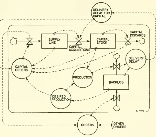
Figure 2.

The

stock

management

system applied to aggregate capital investment.

The model

portrays a firm

which

produces capital plant and equipment.

The

demand

for the firm's product

is exogenous, as is the delivery delay for acquiring

new

capital stock.

When

the self-ordering

multiplier is introduced, the firm's

own

orders for capital add to the

exogenous demand,

and

the delivery delay for capital

becomes

the firm's

own

delivery delay.

SUPPLY

UNE

CAPITAL ACQUISITIONS

CARTAL

STOCK N _CAPITAL ^ DISCARDS

o

/

S^

( DELIVERY

L

ill

DELAY 7 fpRooucnoNj

\

_J

BACKLOG

K-not _

-/OTHER

\ORDERS

D-3921

31

Figure 3. Typicalresultsofthe macroeconoinic experiment.

4

iitKaMaMMMMMa

D-3921

35

Trial

Table 2.

Macroeconomic

experiment: Estimated parameters.

Score

as

Std. Error*

asL

Std. Error* R2 Mode

1200n

1000-Gome18

600

100

Figure 4. Simulation ofthedecisionrule with estimated parameters.

eoo Proaucllon Capacity 1200 HOOn 1200 1000 600 Game36 800 Production CapecUij

*

1200 eoo 750 c TOO o o a. ^ 600 •> o 550 500 150 Game 12 500 600 700 Production Capacity eoo 880 1230 1250 Production Capacity 1270 1200-1 Game 10 100 800 ProductionCapacity 1200

D-3921

35

a

Figure 5.

Modes

ofthe system inparameterspace.

Lower

graph

zooms

into areabetween (0,1).

D-3921

37

Figure7. T^'picalexperimentalresults oftheBeerdistribution

Game.

7a:

Customer

Orders. In

week

5customerordersrise

from

4 to 8 cases perweek.

Compare

against the oscillations inthe subjects'orders(7c).

30-25 - ro15 -'J -5

-Figure7b.

Key

toexperimental results (figure 7c).

a

Factory ^ Distributor

_ Wholesaler

Retailer

Orders placed bysector.

Frombottom totop,

R. W.D,F,eachoffsetby15cases/week. Major tick-marks=l5 cases/week. Minortick-marks=5 cases.'week

Initialorders=4cases/weekinallsectors.

5 10 U 20 25 30 :5 Weeks o c 01 > c o o Factory Distnbutor Wholesaler Retailer

Effective Inventoryby seaor.

Effective lnventory=lnventory-Backlog.

Frombottomtotop,

R, W.D, F,eachoffset by40cases. Maior tick-marks=40cases. Minor tick-marks=lOcases.

Initial inventorysl2casesin allsectors.

3 10 13 20 23 30 33