Emna Nefzi
H05263
Master of Science at HEC Paris Specialization: Finance
Subject of the thesis:
Valuation of Continuous Asian Options: Comparison of Laplace Transform Inversion method with Monte Carlo Simulation
Thesis directed by Professor Laurent Calvet
May 22, 2009 Jouy-en-josas, France
VALUATION OF CONTINUOUS ASIAN OPTIONS:
Comparison of Laplace Transform Inversion method with Monte Carlo Simulation
ABSTRACT
Finance provides mathematics with challenging problems to be solved. Among them Asian options, i.e. options whose payoff depends on the average price of the underlying asset, that have characteristics such as their valuation requires the use of approximation techniques as, to this date, there is no known closed form analytical solution for arithmetic average options. Hence, different attempts to price average value options have been completed through various approaches (analytical approximation, binomial trees, Monte Carlo simulation...etc).
In this thesis, we focus on one of the analytical methods, Laplace transform, developed initially in 1993 by Geman and Yor and extended later in different new modelling approaches. We realize an analysis of the results given by such method using the software Mathematica 7.0.1, using Monte Carlo simulation as a control variable and comparing the set of our results with the outputs from several numerical approximation techniques extracted from the existing literature on average options.
Keywords: Option pricing; Asian option; Laplace transform; Mathematica; Monte Carlo simulation
AKNOWLEDGMENTS
I would like to thank Professor Laurent Calvet of HEC Paris Business School for directing this thesis. He provided me with valuable commentaries as to the orientation of my research
approach and devoted time for that purpose despite his busy schedules. Moreover, I congratulate him for the issue of his book Multifractal Volatility: Theory, Forecasting and Pricing and in the end, I will conclude by re-expressing my thankful and respectful thoughts.
CONTENTS
1. INTRODUCTION: ...7
2. ASIAN OPTIONS: GENERAL PRESENTATION:...8
2.1. EXOTIC OPTIONS: ...8 - Rainbow options:... 8 - Binary options: ... 9 - Barrier options:... 9 - Look-back options:...10 - Asian options:...12
2.2. ASIAN OPTIONS: GENERAL CHARACTERISTICS: ...12
2.2.1. Average rate options:... 12
2.2.2. Hedge ratios using Monte Carlo simulation:... 13
2.3. CLASSIFICATION OF ASIAN OPTIONS:...14
- Geometric Asian options and arithmetic Asian options:...14
- Average Strike Options (ASO) and Average Price Options (APO):...15
- In Progress averaging option and Forward-starting option: ...15
2.4. REASONS FOR THE POPULARITY OF ASIAN OPTIONS: ...16
- Providing competitive prices:...16
- Lessening price manipulation:...16
- Hedging balance-sheet:...16
3. VALUING ASIAN OPTIONS: ... 17
3.1. GENERAL FRAMEWORK: ‘CLASSIC’ ASSUMPTION OF A GEOMETRIC BROWNIAN MOTION:...17
3.2. LITERATURE OVERVIEW: SELECTION OF FUNDAMENTAL ARTICLES ON THIS FIELD: ...19
- Kemma and Vorst (1990)...19
- Geman H. and Yor M. (1993) ...20
- Bouaziz, Briys and Crouhy (1994)...21
- Cruz-Baez and Gonzalez-Rodriguez (2007)...22
3.3. OBSTACLES FOR PRECISE PRICING OF ASIAN OPTIONS: ...23
3.4. PRICING METHODS:...23
- Turnbull & Wakeman (TW): ...23
- Shaw: ...24
- Post-Widder (PW): ...24
4. ASIAN OPTIONS PRICING METHODS STUDIED: ...25
4.1. LAPLACE TRANSFORM: ...25
4.1.1. Description of the method of Laplace transform: ... 25
4.1.2. Application of Laplace transform method for the specific case of Asian options:... 26
4.1.3. Implementation of Laplace Transform technique in Mathematica 7.0.1: ... 28
4.2. NUMERICAL BENCHMARK TECHNIQUES: MONTE CARLO SIMULATION AND EULER...29
APPROXIMATION: ...29
4.2.1. General presentation of the method of Monte Carlo simulation:... 29
4.2.2. Euler Approximation Schemes: ... 31
- Standard schema: ...31
- The Euler schema as proposed by Abate and Whitt: ...31
4.3. NUMERICAL RESULTS AND COMPARISON: ...33
4.3.1. Initial parameters:... 33
4.3.2. The outputs of the numerical approximations through Mathematica: ... 34
4.3.3. Comparison with other methods:... 38
5. CONCLUSION:... 41
LIST OF TABLES
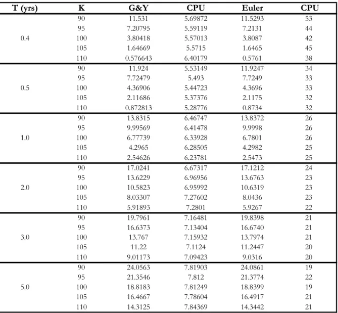
TABLE 1: Numerical results: Inverting the Geman & Yor (G&Y) Continuous Asian Call
Option Laplace transform using Mathematica and their required calculation time… ... 34
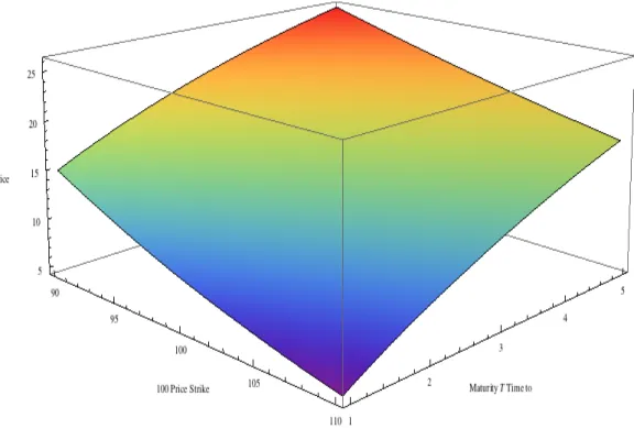
FIGURE 1: Pricing a continuous Asian call option given the Laplace transform technique for σ
= 10% with different range of parameters (ie. K ∈ [90,110], T ∈ [1,5]). ...35
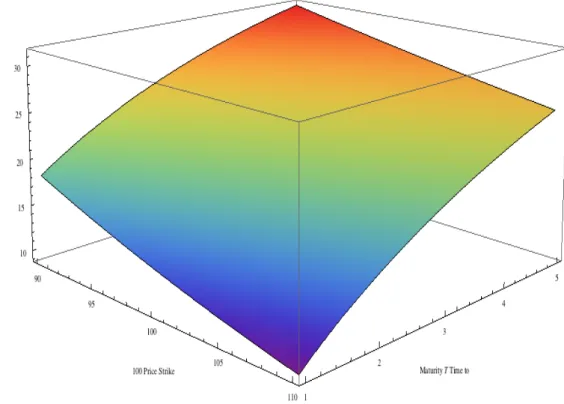
FIGURE 2: Pricing a continuous Asian call option given the Laplace transform technique for σ = 30% with different range of parameters (ie. K ∈ [90,110], T ∈ [1,5]). ...36
FIGURE 3: Pricing a continuous Asian call option given the Laplace transform technique for σ
= 30% with different range of parameters (ie. K ∈ [90,110], T ∈ [1,5]). ...37
TABLE 2: Numerical results comparison: Inverting the Geman & Yor (G&Y) Continuous
Asian Call Option Laplace transform using Mathematica and comparison with other
approximation technique results and the Monte Carlo simulation outputs... 38
TABLE 3: Calculation time comparison... 40 APPENDIX A: Mathematical proof of the simplified expression of a continuous call option as
demonstrated by Geman & Yor ... 42
APPENDIX B: Algorithm for Mathematica7.0.1 based on the inversion of Laplace transform
SYMBOLS & ABBREVIATIONS
S(t) The price of the underlying asset at instant t
A(t) The average price of the underlying asset S(t) observed over the period [t0,T]
K The strike price
r The risk-free interest rate
T The maturity time
t0 The starting instant for the calculation of the average
Wt The geometric Brownian motion
σ Volatility of the underlying asset
N(.) The cumulative normal distribution function
N The number of samples considered in the case of a discrete average
Ct,T The price of a European Asian option at a time instant t with maturity T
PDE Partial Differential Equation s Laplace variable
v Index of a Bessel function F t Continuous filtration
G&Y Geman & Yor G&E Geman & Edyeland
MC Monte Carlo
PW Post Wider
1. Introduction:
Among the long list of exotic assets such as lookback, compound, knock-out and balloon options, Asian options also called average rate options have been for years one of the most popular form of exotic options. Historically, they have been called “Asian options” because Bankers Trust who was the first to offer such products (in 1987) offered them initially in their Tokyo office.
In fact, Asian options are defined as path-dependent options whose payoff is based on the average price of the underlying asset. Hence, at maturity (t=T), the payoff function equals the following equation:
Max A(T )!
[
!!K,!0]
=! A(T ) ! K(
)
+!where A(T) denotes the average price of the underlying asset S(t) observed over the period. Even though the average price may be computed as either a geometric average or as an arithmetic average, practitioners widely use arithmetic averages in the market place despite the non-existence of a closed form solution for the price of an arithmetic average price option. Consequently, in a framework of continuous stochastic variable, an arithmetic average is calculated as shown in the following equation:
A(x)!=! 1 x! t0 ! S(u)!du t0 x
"
The reason for the difficulty of pricing such options comes indeed from the fact that the distribution of the arithmetic average of a set of lognormal distributions, not only does not have a lognormal distribution, but also does not have any analytically tractable properties and
therefore, no one has been able to produce an exact formula for this arithmetic average of lognormal stochastic variables.
Hence, as their pricing models still requires important improvements, a swarm of researchers from academia and the industry have churned out a number of closed form approximations for arithmetic average options and there seems to be no end to the interest in improving their approximation.
2. Asian options: General presentation:
The class of standard European and American call and put options (known also under the naming of plain vanilla options) are actively traded in financial markets and are quoted by
exchanges or by brokers on a regular basis. We remain at this stage that a call option (respectively a put option) is defined as a contract that gives the holder the right to buy (resp. sell) the
underlying asset by a certain date for a certain price.
Plain vanilla options have standard characteristics and have well known estimated values (set under various famous pricing models such as the classical framework of the Black & Scholes model for example) and can indeed be traded either over the exchange-traded markets and/or the Over-The-Counter (OTC) markets for equities, fixed income, foreign exchange and commodities.
Nevertheless, such standard instruments do not necessarily fit with the numerous objectives and divergent hedging issues of the panoply of actors present in the financial industry (traders, corporate treasures, fund managers...etc).
Hence, in order to customize the existing products so that they meet the specific needs of investors, many variants have been created and added in to the former characteristics of plain vanilla option contracts. Indeed, the financial engineers have shown such wide and imaginative ideas that the number of various specific new types of options (that will be categorized under the class of exotic options) have reached an impressively high level and detain all the needed features that the investors were looking for initially. But one famous example among exotic options is indeed given by Asian options that are deepened in this thesis. Therefore, before starting
developing their properties and characteristics, we would like to start underlining some examples of other types of exotic options (focusing mainly on their valuation method).
2.1. Exotic options:
The list of exotic options is very long and small-added variants that customize each class of them can be infinitely included each time. Hence, far from giving an exhaustive list of the available exotics traded on the OTC markets, the aim of this section is to give some famous examples of exotics and see particular methods of valuation that have been applied to them.
Consequently, among the different categories1 of exotics, we give the following
examples:
- Rainbow options:
The term rainbow option is applied to an entire class of options that are written on more than one underlying asset. Rainbow options are usually calls or puts on the best or worst of n underlying assets. Indeed, such options are used an efficient tool for hedging the risk of multiple assets and as a matter of fact, give the same features as a correlation trade, since the value of the option is sensitive to the correlation between the various basket components.
1 With the term ‘categorization’ of the different existing classes of exotics, we refer indeed to the classification found in the
Hull book titled Options, Futures and Derivatives, that relies itself on the categorization set between 1991 and 1992 in the range of articles written by Eric Reine rand Mark Rubinstein for Risk Magazine.
Concerning the pricing issue, rainbow options are usually priced using an appropriate industry-standard model (such as Black-Scholes) for each individual basket component, but in addition to that a matrix of correlation coefficients must be applied to the underlying stochastic drivers for the various models. While degenerate cases have simpler solutions, the general case must be simply approached with Monte Carlo methods.
- Binary options:
Such options, known also under the name of digital options (more common in forex/interest rate markets) or also Fixed Return Options (FROs) on the American Stock Exchange, are named binary options because there are only two possible outcomes for their payoff function. In fact, these options have a fixed payoff if the option ends up being in the money at expiration, regardless of the extent to which it is in the money, and at the opposite, worth nothing if the option ends up out of the money.
Hence, this type of option has the specificity of presenting a discontinuous payoff function that can take only two possible outputs: either the payoff is some fixed amount of some asset or the options worth nothing at all.
Besides, depending on the nature of the fixed payoff at maturity, we split generally the binary options into two types of groups: the cash-or-nothing binary option on the one hand, and the asset or nothing binary option on the other hand. The cash-or-nothing binary option pays some fixed amount of cash if the option expires in the money, while in parallel the asset-or-nothing option pays the asset price if it ends up above the strike price.
- Barrier options:
A barrier option is similar to a plain vanilla option but with one difference: in addition the “classical” features of a plain vanilla option, there exist one or two “trigger prices”. If the barrier or the “trigger” price is reached at any time before maturity, it causes an option with pre-determined characteristics to come into existence (in the case of a knock-in option) or it will cause an existing option to cease to exist (in the case of a knock-out option).
Accordingly, there exist 8 types of barrier options:
- A down-and-out call option (a call option that ceases to exist if the asset price reaches a certain barrier level H that is lower than the initial asset price)
- A down-and-in call option (a call option that comes to existence if the asset price reaches a certain barrier level H that is lower than the initial asset price)
- An up-and-out call option (a call option that ceases to exist if the asset price reaches a certain barrier level H that is higher than the initial asset price)
- An up-and-in call option (a call option that ceases to exist if the asset price reaches a certain barrier level H that is higher than the initial asset price)
- A down-and-out put option (a put option that ceases to exist if the asset price reaches a certain barrier level H that is lower than the initial asset price)
- A down-and-in put option (a put option that comes to existence if the asset price reaches a certain barrier level H that is lower than the initial asset price)
- An up-and-out put option (a put option that ceases to exist if the asset price reaches a certain barrier level H that is higher than the initial asset price)
- An up-and-in put option (a put option that ceases to exist if the asset price reaches a certain barrier level H that is higher than the initial asset price)
Here, we consider just the examples of a down-and-in and a down-and-out call options. The other options have similar valuation expressions that have been derived from the same methodology.
Indeed, it has been proved that for a down-and-out call option, the valuation expression is the following:
Cdown!and !in(t)!=!S0e
!qT(H S 0) 2" N(y)!!!Ke!rT( H S0) 2" !2N(y!# T ) where!"!=!r! q + #2 2 #2 !and!y!=! ln H2 (S0K ) $% &' # T !+!"# T
Thus, based on the former equation and considering the fact that a standard call option can be compounded by two barrier call options as:
C(t)!=!Cdown!and !in(t)!+!Cdown!and !out(t)
Hence, it is easy to derive an expression for the down-and-out call option through subtracting a down-and-in call option price from the price of the standard corresponding call option, simple operation that leads to the following expression:
Cdown!and !out(t)!=!S0N(x1)e
!qT ! Ke!rTN(x 1!" T )!!!S0e !qT(H S 0) 2#N(y 1)!+!Ke !rT( H S 0) 2#!2N(y 1!" T ) Where!x1!=!ln(S0 H ) " T !+!#" T !and!y1!=! ln(H S0) " T !+!#" T - Look-back options:
Look-back options constitute one category class of the large family of path dependent options. They give indeed their owners the right to buy or sell the underlying security at the most attractive price (buy at the low and sell at the high). Consequently, they are attractive to investors but are, at the same time, more expensive than their corresponding plain vanilla options.
Indeed, like for the case of Asian options, there are two types of look-back options:
♦ Look-back options with floating strike price:
In this case, the strike price is replaced by the most attractive price of the underlying asset (lowest for a call and highest for a put). Hence at maturity, the payoff function is equal to:
Max 0!,!S(T )!!! Min t" 0,T[ ]S(t) # $% &'(!! for!a!call and! Max 0!,! Max t" 0,T[ ]S(t)!!!S(T ) #
$% &'(!! for!a! put ! ) * + + , + +
In 1979, a closed form analytical expressions have been found to valuate these options2 and we show below their corresponding expressions (S
min denotes the
lowest price achieved to date and Smax the maximum one):
For a call, the price of the option is:
C(t)!=!S0e !qTN(a 1)!!!S0e !qT "2 2(r! q)N(!a1)!!!Smine !rT N(a 2)! "2 2(r! q)e Y1N(!a 3) # $ % & ' ( where!a1!=! ln(S0 Smin)+ (r ! q +" 2 2)T
" T ,!a2=!a1!" T ,!a3!=!
ln(S0 Smin)+ (!r + q +" 22)T " T !and!Y1= !! 2(r! q !"22)ln(S 0 Smin) "2 Symmetrically, for a put, we have the following expression:
P(t)!=!Smaxe !rT N(b1)! "2 2(r! q)e Y2N(!b 3) # $ % & ' (!+!S0e !qT "2 2(r! q)N(!b2)! S0e !qT N(b2) where!b1!=! ln(Smax S0)+ (!r + q +" 2 2)T " T ,!b2=!b1!" T ,!b3!=! ln(Smax S0)+ (r ! q !" 2 2)T " T !and!Y2=! 2(r! q !"2 2)ln(Smax S0) "2
♦ Look-back options with fixed strike price:
In the case of a fixed strike price, the payoff function at maturity equals:
Max 0!,! Max t! 0,T[ ]S(t)!"!K # $% &'(!! for!a!call and! Max 0!,!K !"! Min t! 0,T[ ]S(t) #
$% &'(!! for!a! put ! ) * + + , + + 2
Proof available in the article “Path-Dependent Options: Buy at the Low, Sell at the High” for the 3 authors M.A.Gatto, H.Sosin and B.Goldman, published in the Journal of finance, 34, pp.1111-27, and in the article “Recollection in Tranquillity” for M. Garman, published in Risk, pp.16-19.
Despite their similarity with the floating look-back options, a valuation method for the fixed look-back options has been found only in 2003 thanks to a put-call parity argument developed in the article “Sub-replicating and Replenishing premium: Efficient Pricing of Multi-state Lookbacks” presented in the Review of Derivatives Research by Y.K. Kwok and H.Y. Wong. These latters proofed indeed that if we denote with:
Smax * = Max(S max, K ) and Smin* = Min(S min, K ) ! " # $ #
and substitute Smax by S*max ad Smin by S*min in the former expressions of the
floating look-back options, we obtain the two following call-put parity relationship:
Cfixed! strike! price(t)=!Pfloating! strike! price(t)+ S0e
!qT ! Ke!rT
Pfixed! strike! price(t)=!Cfloating! strike! price(t)! S0e
!qT + Ke!rT
- Asian options:
Asian options are among the most popular class in the exotic and path-dependant options family and in the opposite to the majority of exotics, they do not have a closed form analytical solution. Therefore, we suggest in this thesis to go deeply into one of the valuation methods that is the inversion of Laplace transform. Further development will be given all long this thesis.
2.2. Asian options: general characteristics:
2.2.1. Average rate options:
As explained above, Asian options are path-dependent options whose payoff is based on the average price of the underlying asset. Hence, at maturity, the payoff function an be expressed as:
Max A(T )!
[
!!K,!0]
=! A(T ) ! K(
)
+!where A(T) denotes the average price of the underlying asset S(t) observed over the period.
Indeed, Asian options appeared quite early in financial markets. Some early examples of underlying assets on which Asian options contracts were set have been provided by Kemna and Vorst through the examples of Mexican Petrobonds in 1977, the example of Oranje Nassau bonds in 1985 where the price is based on the average Brend Blend oil price over the last year of the contract and the Delaware Gold indexed bond, based on the average gold price over 10 trading days3.
3 Examples extracted from the article A Pricing Method for Options Based on Average
2.2.2. Hedge ratios using Monte Carlo simulation:
The hedging issue of different types of underlying densities like the ones with non-normal returns (matter consistent with the case of discrete Asian options) has been discussed for the first time in the empirical literature of Mandelbrot (1963) and Fama (1965). Nonetheless, a more complete method for the calculation of hedge ratios have been proposed only in 1992 by Carverhil and Clewlow who proposed to approximate the partial derivative by the centred difference equations and then apply the Monte Carlo simulation to estimate them.
Hence for the various Greek letters, the centred difference equation can be applied as illustrated by the following:
- Delta that is estimation of the change in the option price as the underlying asset changes can be simulated as following:
!!=!"C "S #!
C(S+$S)!%!C(S %$S)!
2$S
- Gamma that estimates the change in delta as the underlying asset changes equals indeed: !!=!"2C
"S2 #!
C(S+$S)!%2!C(S)!+!C(S % $S)! ($S)2
- Vega which is defined as the rate of change in the option price with respect to volatility can similarly estimated by the following:
V !=!!C
!" #!
C(" +$")!%!C(" %$")! 2$"
- And finally Theta that permits to follow the change in the option price as time to expiration changes is estimated as:
!!=!"C "t #!
C(t+$t)!%!C(t)! $t
It is easy based on the valuation expressions of these Greek letters to apply a Monte Carlo simulation to obtain an estimation of their levels based on a range of simulations of random paths of the underlying asset. Nevertheless, in addition to the Monte Carlo simulation, many techniques have been applied to the hedge ratios of Asian options and some explicit formulas for the hedging portfolio have been suggested using the usual lognormal approximation method or the inverse Gaussian approximation…etc.
2.3. Classification of Asian options:
The most generalized and frequent classification of options consists in separating two cases: the discrete and continuous pricing. This categorization applies for average options too. Indeed as underlined by M.C. Fu and D.P. Madan, “if the average is computed using a finite sample of asset price observations taken at a set of regularly spaced time points we have a discrete Asian option, on the contrary a continuous Asian option is obtained by computing the average via the integral of the price path over an interval of time”4.
But, in addition to this general classification, more specific criteria to sort average options have been used in the literature and we find usually:
- Geometric Asian options and arithmetic Asian options:
The average can be calculated in two different ways, either using a geometric mean or an arithmetic mean (that is more commonly used).
Let’s S(ti) denote the evolution of the underlying asset, observed at different instants
ti, where i=1,2…N and if I equals N, we obtain tN equivalent to maturity instant T.
Hence, we can define the average in each case as following: The Arithmetic average:
In the discrete case:
To elaborate on arithmetic averaging, this is seen in the discrete case as being the sum of the sampled asset prices divided by the number of samples:
A(T )!=!1
N i=0S(ti) N
!
In the continuous case, we obtain the following average: A(T )!=! 1 T ! t0 ! S(u)du t0 T
"
The Geometric average:
For geometric averaging, the average value is taken as (N+1) root of the sample values multiplied together:
A(T )!=! S(ti) i=0 N
!
" #$ % &' 1 N+14 Extracted from Pricing Continuous Asian Options: A Comparison of Monte Carlo and Laplace Transform Inversion Methods, written by Fu, M.C, D.B. Madan and T. Wang in the Journal of computational finance, vol.2(2), p49-74, 1999.
- Average Strike Options (ASO) and Average Price Options (APO):
Dependently on the nature of the contract set between two counterparties, a contract on an Asian option can have (or not) a fixed strike price. Hence, there exist two types of average options in the financial markets:
Options with fixed strike price:
In the case where the strike price is determined ex-ante (among the other characteristics of the contract), the option is in this case called an Average Price Option and the payoff function depends at a specific instant t ∈[0,T] on four parameters S(t), A(t), K and t. Hence, at maturity, the payoff function equals:
Max A(T )!
[
!!K,!0]
=! A(T ) ! K(
)
+! Options with floating strike price:
In few cases, the strike price can be floating and the payoff function depends hence only on three parameters S(t), A(t) and t. Such option is less widely used in practice and is indeed known as an Average Strike Options. Consequently, at maturity, the payoff function equals:
Max S(T )!
[
!!A(T ),!0]
=! S(T ) ! A(T )(
)
+!- In Progress averaging option and Forward-starting option:
An Asian option will be considered as “in progress averaging” option if the calculation of the average starts when the contract is established. This means that partial information on the value of the option at maturity is been immediately revealed with the creation of the contract.
On the contrary, in the case of a forward starting option, the calculation of average does not start immediately with the establishment of the contract but starts at a later instant (the starting moment of the calculation of the average is determined and set as one of the characteristics of the contracts). Hence, for forward starting Asian options the time to maturity period is always larger than the time period needed for the calculation of the average.
2.4. Reasons for the popularity of Asian options:
Asian options are traded Over-The-Counter and are very popular in the financial community that frequently uses them as options on oil or options on spreads between two types of oils. The reasons for their popularity are numerous and can be divided principally into three categories:
- Providing competitive prices:
One is attempted to think that Asian options have a lower volatility (as considered on the average value of the underlying asset) and indeed this feature renders them cheaper relative to their European counterparts. Moreover, many authors have underlined this fact until a more precise statement presented with a complete mathematical proof by Geman & Yor emphasized the conditions to the validity of this assumption.
The co-authors actually pointed up that “in contrast with most of what has been written so far, an Asian option may be more expensive than the standard option”. In fact, they showed that an Asian call option is cheaper than its European corresponding option if for example the underlying asset is a domestic stock. Nevertheless, for some specific cases (i.e. the case where the index of the Bessel process is strictly lower than one), the price of the Asian option “ is greater than the standard option price for all the values of the exercise price K in a neighbourhood of 0). Hence, we underline the fact that the advantage of the price attractiveness is valid only under some conditions.
- Lessening price manipulation:
Asian options allow lessening the risk of price manipulation. In fact, let’s examine the following situation: we consider the case of a specific illiquid market where there exist players detaining important sized positions. The risk of a price distortion that may appear because of the lack of depth of such market remains likely to appear. If the option payoffs are determined by the price of the underlying asset on a particular day, price manipulation is always possible through the effects of price impact.
Hence, if we set now an agreement in which the payoff of the options will depend -not on the level of the underlying asset at a specific moment- but rather upon the average closing price of the asset over a six-month period for example, it would be much more difficult to profit from any sort of manipulation.
Indeed, the low sensitivity of the Asian options to movements of the underlying asset price when the option is close to maturity permits to lessen price manipulation as the weight of the asset fluctuations during the closing period are small in comparison with the weight of the underlying asset fluctuations for the overall period.
- Hedging balance-sheet:
Asian options permit to meet some needs for corporate treasurers who are increasingly interested in having an average rather than year-end rate to hedge the exposure in the balance sheet.
Moreover, as stated by Geman and Yor, Asian options are a “less expensive means for corporations to hedge a series of risky positions on the foreign exchange incurring at a steady rate over a period of time”5.
For example, a US corporate treasurer who registers Euro inflows over one year from a French subsidiary is highly interested in having an option that guarantees an average exchange rate Euro/US over the whole period rather than registering the operations with different rates that eventually have heterogeneous levels. Asian options can guarantee such operations and can insure that the average exchange rate realized during the year remains above some level.
3. Valuing Asian options:
3.1. General Framework: ‘Classic’ assumption of a Geometric Brownian motion: Among the central hypotheses considered for the majority of asset price modelling assumptions, the Brownian motion is certainly the commonly agreed central point of the mathematical framework and is more generally considered as the “ workhorse of continuous time finance theory”6.
In fact, the geometric Brownian motion, introduced since 1964 into the study of stock market prices by Osborne, has been indeed imported as many other financial concepts from the domain of physics and particularly from the description of the motion of a heavy particle suspended in a medium of light particles that occasionally randomly crash into this latter and hence displaces it. The similitude in finance with this physical phenomenon has been derived from the fact that stock prices (i.e. heavy particles) are impacted by trades (i.e. light particles) and this statement can be linked actually to the whole theory that will be developed later on how order flow (trades) moves stock prices (theory of informational efficiency of financial markets)7.
From a mathematical view, a stochastic process S(t) is said to follow a geometric Brownian motion if it satisfies the following stochastic differential equation:
dS(t)!=!rS(t)!dt!+!!S(t)!dWt
5 H. Geman and M. Yor, Bessel processes, Asian Options and Perpetuities, Mathematical Finance, 3 (1993), pp.349-375. 6 Calvet, Laurent E., and Adlai J.Fisher (2008), Multifractal Volatility : Theory, Forecasting and Pricing. Elsevier –
Academic Press.
7 To deepen this subject, we refer the reader to the book of Thierry Foucault, Bruno Biais and Pierre Hillion,
«Microstructure des Marchés : Institutions, Modèles et Tests Empiriques», Presses Universitaires de
For example, the following graphs shows 50 possible trajectory of a stochastic variable S(t) that follows a geometric Brownian motion:
Given the important consequences of the hypothesis of Brownian motion on the properties that will characterize the prices of the underlying asset, we will develop in detail the properties of such motion and indeed we separate them into these six main
characteristics8:
a. Property of finiteness: Any other scaling of the bet size or increments with time step would have resulted in either a random walk going to infinity in a finite time, or a limit in which there was no motion at all. It is important that the increment scales with the square root of the time step.
b. Continuity: the paths are continuous. There are no discontinuities. Brownian Motion is the continuous time limit of our discrete time random walk.
c. Markov characterization: The conditional distribution of X(t) given information up until h<t depends only on X(h)
d. Martingale property: Given information up until h<t the conditional expectations of X(t) is x(h)
e. Quadratic variation: if we divide up the time 0 to t in a partition with n+1 partition points t(i)=it/n then X(tj)!!X(tj!1)
(
)
j=1 n"
2 !#!t!!almost!surely.f. Normality: Over finite time increments ti-1 to ti, we have X(ti)-X(ti-1) is normally
distributed with mean zero and variance ti - ti-1.
8 This classification has been extracted from the Wilmott Paul’s development on the properties of the geometric Brownian
The impacts of using the assumption of a geometric Brownian motion are very important in modelling the behaviour of the underlying asset and indeed this assumption has been considered as one of the most basic and fundamental pillar for the pricing models developed for the majority of options (including the class of Asian options). We remind finally that the solution for the stochastic differential equation of the geometric Brownian motion process is well know and proved to be equal to:
St!=!S0 !e !(r! "2
2 )s !+!"Wt
3.2. Literature Overview: Selection of fundamental articles on this field:
Asian options have been the subject of continuous scholarly investigation that covered various features of methodologies applied for pricing models and that can be basically categorized into the main following methods:
• Analytical approximations
• Partial differential equation approach • Binomial trees and lattices
• Monte Carlo Simulation
• Pseudo-analytical characterizations.
In this section, we develop a general overview of central articles that have been considered as a pillar of the existing literature. Indeed, in spite of the large number of academic references available on Asian options, we decided arbitrarily to focus only on a limited number of them in order to favor a synthetic analysis and center attention on the fundamental points of the subject. The organization of this section is set with regard to an historical classification of major academic contribution.
- Kemma and Vorst (1990)
In their paper titled A Pricing Method for Options Based on Average Asset Values, the two authors Kemna and Vorst emphasize the fact that it is impossible to derive an explicit formula for Asian options. They give besides a mathematical proof of the fact that Asian options are necessarily and in all cases lower than (or equal to) to the price of a standard European option (indeed, few years later M.Yor will reconsider and refine this assessment, certifying its validity only under certain conditions).
Hence, with regard to what have been said, Kemna and Vorst proposed a simple method for giving a lower bound for average value options based on the geometric average rather than the arithmetic average9. In fact, considering the geometric average
allows, on the one hand, lowering considerably the complexity level of the problem (as the geometric average of lognormally distributed variables is indeed lognormally distributed too) and, on the other hand, providing a closed form analytic solution for Geometric averaging options.
9 Using the geometric average rather than the arithmetic average leads necessarily to an under-pricing of the options since a
The solutions to the geometric averaging Asian call is given as: C(K )!=!e 1 2(r! 1 6" 2)(T!t 0) S(t0)!N(d1)!!!K !N(d2)
Where N(x) is the cumulative normal distribution function of:
d1!=! log(S(t0) K )!+! 1 2(r+ 1 6! 2 )(T" t0) ! 1 3(T" t0) and, d2=!d1!!!" 1 3(T! t0)
- Geman H. and Yor M. (1993)
Geman and Yor presented in 1993 a highly interesting work in the domain of mathematical finance as they showed a new technique to price Asian options thanks to the inversion of Laplace transform. In their article named Bessel Processes, Asian Options, and Perpetuities, the co-authors underline the fact how Bessel processes can help solving several problems involving the integral of an exponential of Brownian Motion.
In mathematics, a Bessel process is a type of stochastic process that constitutes one parameter family of diffusion process. This type of process appears in many financial problems and has remarkable properties. Indeed, in section 3.1, we have seen another type of diffusion process commonly considered for pricing financial instruments and widely known as the basic assumption in the Black and Scholes pricing model, which is the geometric Brownian motion. Similar to this latter, the Bessel process squared (BESQ)10 is also a continuous diffusion process that satisfies the following stochastic
differential equation:
d!t!=!"!dt !+!2 !t!dWt
where Wt denotes - like in the case of a geometric Brownian motion – a standard one
dimensional Brownian motion.
Hence, using stochastic calculus and several tractable properties of Bessel
processes, Geman and Yor obtained an analytical formula for the Laplace transform of an Asian call option. Actually, the method applied by the co-authors is the core subject of this thesis and we will explain further the different steps followed to obtain the analytical formula driven by the Laplace Transform method and its implementation in the
computation software Mathematica.
10
We give here the definition of a “ Bessel process squared” (BESQ) and not the definition of a “Bessel process” (that we denote BES and that is simply the square root of a Bessel process squared) to avoid long notation.
Besides, we will compare the outputs of our algorithm with the results found in the Geman and Edyeland article11 (which was the first article to present numerical
examples of results obtained from Geman and Yor’s theoretical work). For more profound study for the accuracy of our results, other approximation methods will be compared also to our outputs as well as the industry benchmark Monte Carlo simulation.
- Bouaziz, Briys and Crouhy (1994)
The idea developed by the three authors in their article12 published in the Journal of
Banking & Finance in 1994 suggests a straightforward solution to overcome the
complexity of the expression of the payoff function of Asian options. In fact, they derive a closed form approximate solution and provide a derivation of a formal upper bound to the approximation error based on the geometric average. Their analysis has the great advantage of presenting a clear and accessible approach, with a non-complex
mathematical proof that the central idea is explained above:
Basically, as we try to understand the behaviour of Asian options’ payoff function, in general we reach quickly a deadlock as its obviously complex expression contains the integral of the exponential of a Wiener process, expression to which no direct handling can be applied. We remind at this stage that the aim of our research is to find tractable properties of the arithmetic average of a stochastic continuous variable that follows the following equation:
St!=!S0 !e !(r! "2
2 )s !+!"Wt
where σ denotes the volatility of the asset and Wt a Brownian motion.
The idea suggests in their article is to use Taylor expansions applied for
exponential, which is the first order linear development of exponential as shown in the following equation:
ex !!1!+!x
And using such a simple linearization procedure leads -after some straightforward computations- to the following approximate closed form solution to the pricing of the Asian Options over the time interval [0,T-A]:
Ct ,T! A(K )!=!St!e (!rA)! ˆr(A 2)!N( 3ˆr A / 2" )!+! " 2A / 6# !e(!3ˆr2A /8"2) $ %& ' ()
where N(.) denotes the univariate cumulative normal distribution, A denotes the time instant at which the underlying asset starts to be taking into account for the average calculation13 and ˆr!=!r !1 2" 2 11
Geman, H. and A. Eydeland, Domino Effect, Risk (8), pp.65-67, 1995.
12 L. Bouaziz, E. Briys, and M. Couchy, The Pricing of Forward Starting Asian Options, Journal of Banking and Finance, 18
(1994),pp. 832-839.
13 Bouaziz, Briyus, and Crouhy considered in their paper the case of forward starting options. As A denotes the instant time
at which the average starts being computed, we look for the computation of an arithmetic average of the underlying asset prices over the period [T-A,T].
Nevertheless, the option used in their paper is an Average Strike Option (ASO or floating strike Asian option) that is less widely used in practice in comparison with the Average Price Option (APO) and the model provided in their paper has indeed been extended to forward starting Asian options. Finally, Bouaziz, Briys and Crouhy provide, based on a comparison with results set thanks to Monte Carlo simulations, an upper bound of the error involved in their linear approximation.
At the end, to be synthetic vis-à-vis the advantages and drawbacks of such method of linearization, there is no doubt that in spite of the fact that the linear approximation allows to give a closed form solution that performs quite well for options with low volatility, the first order linear development (of the exponential of a Wiener process) looses completely its precision and turns to be non-reliable for options that have fluctuations above a certain level of volatility. Some research work done on the break-even volatility level14 that preserves the reliability of the approximation applied by
Bouaziz, Briys and Crouhy estimates in fact this latter to be around 35%. Hence, in the case of the existence of a ‘volatility shock’ on financial markets (like the high volatility observable ones during 2007/ 2008), this linearization method would become obviously obsolete and be an erroneous attempt to price Asian options.
- Cruz-Baez and Gonzalez-Rodriguez (2007)
One of the recent and important methods for pricing arithmetic Asian option (that has been published in a brief paper in the Applied Mathematics Letters in May 2007) has indeed the advantage of presenting an innovative and interesting approach for
valuating Asian options.
The two authors Cruz-Baez and Gonzalez-Rodriguez used indeed the Laplace transform technique but with an approach different from that used by Geman and Yor with Bessel processes in 1993. In fact, instead of using different properties of Bessel process to simplify the expression of the payoff function of Asian options in order to be able to extract a close-form expression for the laplace operator, the authors rely on a different approach that leads to the same solution without using any property of Bessel processes.
What we have seen until this stage is that the majority of the analytical solutions proposed by the various academicians are based on the direct manipulation of the payoff function of Asian options which is:
Ct ,T(K )!=!e !r(T !t )!E Q (A(T )!!!K) + F!!! t "# $%!
Nevertheless, Cruz-Baez and Gonzalez-Rodriguez based their valuating method not on the direct improvement of the function above but indeed worked on the
simplification of the Partial Differential Equation (PDE) of an Asian option and applied the Laplace transform technique for this latter.
14 Such research work can be found in the thesis of Rafal Wojakowski, Evaluation des Options Asiatiques, directed by Marc
Chesney, at HEC in 1992. The research work includes a comparison of the estimation error related to the differences between options prices based on the three following methods: Monte Carlo, the linearization method and a corrective method of the linear approximation (that includes more terms in the approximation of the exponential).
Indeed, the methodology they use is quite understandable and relies on two short steps:
1. First, making an «appropriate change of variables to obtain a suitable partial differential equation ».
2. Second, solving « the partial differential equation via the Laplace transform and Mathematica ».
3.3. Obstacles for precise pricing of Asian options:
Adopting the usual framework initially set in the Black &Scholes model, we suppose that the price of the asset follows a lognormal distribution continuous in time. The difficulty arises for the case of Asian options because the sum of the lognormal variables is not
lognormal, and therefore the distribution cannot be given explicitly and the Black–Scholes method cannot be applied.
This difficulty is expressed differently if we consider the Partial Differential Equation (PDE) that the value of an Asian arithmetic call option satisfies:
!!C !A!+! !C !t !+! 1 2" 2 S2!! 2 C !S2!+!(r # q)!S !C !S!#!rC!=!0
The difference observable in such PDE is that in addition to differentiating with regard to S and t (as for a plain vanilla call option), the complexity of the PDE of an Asian call option comes from the presence of an extra term in this equation in which we
differentiate the price of the call with regard to the unknown average A.
3.4. Pricing methods:
In this thesis, we focus mainly on two pricing methods that are developed in details in the coming sections (Inversion of Laplace Transform and Monte Carlo simulation).
Nevertheless, other pricing methods have been selected from the existing literature to verify the accuracy of our results and compare the speed of calculation of the algorithm that we implement in Mathematica. Therefore, we devote the following section to present the different pricing methods that will be considered as a quick crosscheck for the results of our calculations with what have been presented in literature:
- Turnbull & Wakeman (TW):
In their article A Quick Algorithm for Pricing European Average Options, Turnbull & Wakeman use an expansion of Edgeworth series to derive a closed-form solution for Asian options. The co-authors emphasize the fact that “while it is very difficult to determine the probability distribution for the average, all of its moments can be readily determined. Thus, an Edgeworth series expansion can be used to approximate the distribution”15. They provide therefore an algorithm to compute the
moments of an arithmetic average and derive an expression for Asian options. The technique they developed can be found as a reference in many articles.
15 Turnbull S.M., and L.M. Wakeman, A Quick Algorithm for Pricing European Average Options, Journal of Financial and
Hence, we extracted the outputs they presented for a fixed range of parameters (r, K, S(0)..etc) to compare them with our outputs.
- Shaw:
Shaw gives examples of implementation methods to evaluate Continuous Asian options in the computational software Mathematica. Particularly, he develops the method based on the first two moments of the distribution and compares the outputs of the suggested algorithm in Mathematica with the results proposed by Geman & Eydeland. In fact, these results on the moments distribution have been initially developed by Hull (1996) and we remind the analytical mathematical
expressions for the two first moments distribution of arithmetic Asian price options: If M1 denotes the first moment distribution and M2 denotes the second moment
distribution, we have that:
M1!=! e(r!q)T ! 1 r! q
(
)
T S0 and, M2!=! 2e((r!q)+"2)T ! 1 r! q +"2(
)
(
2r! 2q +"2)
T2 S0 2 !+! 2S0 2 ! r! q(
)
T2 1 2 r(
! q)
+"2!!! e(r!q)T r! q +"2 # $% & '( Then assuming that the average of the underlying asset follows a log-normal distribution, an Asian option can be then priced as an option on Futures contracts and so, we apply directly the analytical mathematical valuation expression for options on Futures contracts in which we plug the following values of F0 and σ:F0!=!M1 and !2 =!1 T!ln M2 M1 2 " #$ % &'
In comparison with the results given by Geman & Eydeland, this implemented method in Mathematica as been judged by Shaw as “quite good for giving rough values” and the algorithm outputs show that “the method gives value close to the exact answer, but may be biased upwards and downwards depending on the parameters”.
- Post-Widder (PW):
The Post-Widder is based on the Post-Widder theorem thanks to which a function f(y) can be approximated by:
fn(y)!=! n+ 1 2ynRn! (!1) k !Re ˆf n+ 1 y (1! R!e " ki /n # $% & '( ) * + , -. k=1 2n
/
Following the recommendation of M.C. Fu, D.B. Madan and T. Wang, we use the PW method “as a check for those cases where it is suspected that numerical
difficulties due to a slowly decaying integrand may arise”16.
4. Asian options pricing methods studied: 4.1. Laplace Transform:
4.1.1. Description of the method of Laplace transform:
The Laplace transform is a mathematical process widely known and very used to simplify complex differential equations or to calculate complicated integrals. Driven initially from probability theory, we can simplify matters in a given equation by applying the Laplace transform to a complex function (the function that we are looking for evaluating and that we denote f) in order to convert it into an algebraic form (that we denote L{f}), which can be solved with relative ease. To attain the answer to the equation or the PDE, we then apply an inverse Laplace transform to the solution of the algebraic equation(s).
To illustrate the Laplace transform, we consider the following example: we have an arbitrary function f(t) that our final objective consists in evaluating it. Indeed, this function f(t) can denote a number of things including a Black-Scholes PDE or a hyperbolic PDE related to black-Scholes, or more importantly the integral of an exponential of Brownian motion in the case of Asian options. Hence, as f(t) is too complex to be evaluated directly, we need to find another function (that we denote L{f} and that is known as the Laplace Transform of f(t)) that is linked to f and that can be more easily evaluated.
Indeed, the generalized relationship that links the function f(t) to its Laplace transform function L{f} is given by the following:
L f (t)
{ }
!=!F(x)!=! ext! f (t)dt 0
!
"
!!!!!!!!!!(4.1)!where L is the Laplace operator of f(t). The term on the furthest right denotes an integral with limits between 0 and infinity.
To obtain the solution to f(t), we inverse the Laplace transform to L{f} as follows:
L!1
{
F(s)}
!=! f (t)!!!!!!!!!!(4.2)
16 Fu, M.C, D.B. Madan and T. Wang, Pricing Continuous Asian Options: A Comparison of Monte Carlo and Laplace
As a matter of fact, we are able to do so because for specific cases, it is simpler to inverse
the whole expression ext f (t)dt 0 !
"
# $ % & ' (rather than trying to find directly an explicit expression for f(t).
At the end, we underline the fact that the Laplace transform becomes particularly useful when we price exotic options and more precisely Asian options as many of the pricing formulas involve the integral of an exponential of Brownian motion which is troublesome to solve directly.
4.1.2. Application of Laplace transform method for the specific case of Asian options: In order to be able to apply the Laplace transform to the payoff function of Asian options, we need to find a simplification of the expression of this latter so that we can express it in a way that allows to find the function L which allows – through its inversion- to find an explicit form for the price of the option.
This is indeed more easily said than done as several theorems and mathematical properties will be needed for such inversion. In this section, we underline with a synthetic methodology the main steps to be followed in order to re-build the schema of the proof set by Geman and Yor (some detailed developments can be found in the appendix A). Hence, given a complete probability space (Ω,F t ,P), we apply the following steps:
1. Starting from the initial point of the payoff function of Asian options which is: Ct ,T(K )!=!e !r(T !t )!E Q (A(T )!!!K) + F!!! t "# $%!
Geman and Yor derived an expression of a continuous Asian call option price and showed that its payoff function can be expressed as:
Ct ,T(K )!=! e!r(T !t ) T ! t0 !4St "2 !C (v) (h, q) Where v!=!2r !2!"!1 h!=!! 2 4 !(T" t) q!=!! 2 4St!(T" t)! K(T " t0)!"! S(u)dut 0 T
#
$ % & '& ( ) & *&and C(v)(h,q) that is defined implicitly in this equation will need to be computed
through the inversion of the Laplace Transform technique.
Indeed, the overall proof of this result can be found in Appendix A through a three-step methodology.
In reality, this first step has been done with the objective of preparing a formulation of the price of an average European call option that allows
determining the function that we denoted f(t) in the section 4.1.1. In fact, we will see further that the function f(t) to which Laplace Transform will be applied refer to C(v)(h,q).
2. Second, as we intend to find the expression of the adequate function L for Asian options (as explained in equation (4.1)), we define hence the function g which designs the Laplace operator of C(v)(h,q), obtaining indeed the Laplace
transform equation for Asian options (replacing in equation (4.1), function f by C(v)(h,q) and function F by g) : g(!)!=! e"!h!C(v) (h, q)dh 0 #
$
!!!!!!!!!!(4.3)3. Then, Geman and Yor derive a close-form expression for the Laplace operator g: g(!)!=! e" x!x(µ"v) 2"2 ! 1
(
" 2qx)
((µ+# ) 2)+1dx 0 1 2q$
! !(
" 2 " 2v)
%(
(
µ" v)
/ 2" 1)
!!!!!!!!!!!(4.4)where Γ denotes the gamma function.
The proof of this result is quite complex and involves precise properties of Bessel processes. Hence, for the complete mathematical proof of this result, we encourage the reader to go back to the central article of Geman & Yor: Bessel Processes, Asian Options and Perpetuities.
This step is indeed important as the obtained expression for g can be easily implemented in Mathematica. The integral present in the expression of function g can be calculated through the numerical approximation function available in Mathematica and named ‘NIntegrate’. Actually, this function usually uses an adaptive algorithm, which recursively subdivides the
integration region as needed and permits such a highly precise approximation for complex integrals (like the expression of g). We underline besides the fact that Mathematica permits to obtain the Euler gamma function directly through using the function “Gamma”.
4. The fourth step consists in making our function regular in the upper-half complex plane. Therefore, we introduce the following function:
!f(h)!=!e!"h
f (h) Hence, we can write that:
!g(!)!=! 1 2" !f(h)!e #!h dh 0 $
%
!!!!!!!!=! 1 2" f (h)!e #(& +!)hdh 0 $%
!!!!!!!!=!g(& + !)5. We obtain then the inverse Laplace transform expression applying the Fourier-Mellin integral formula:
!f(h)!=! 1 2!i e "h!g(" )!d" #i$ i$
%
!!!!!!!!!!(4.5) or equivalently, !f(h)!=! 1 2! e i"h!g(" )!d" #$ $%
!!!!!!!!!!!!(4.5)6. Finally, as we obtained numerically the value of !f(h), it is easy to drive consequently the value of C(v)(h,q) as
C(v)(h, q)!=!e!h!f(h)!!!!!!!!!!(4.6)
As a conclusion, we obtained this way the price of a continuous Average European call option as we remind the obtained expression in Step n°1 of an Asian call option:
Ct ,T(K )!=! e!r(T !t ) T ! t0 !4St "2 !C (v) (h, q)
4.1.3. Implementation of Laplace Transform technique in Mathematica 7.0.1: We use Mathematica 7.0.1 that is the 2009 released version of Mathematica. Mathematica is indeed a fully integrated technical computing software permitting the calculation of complicated integrates through their numerical approximation.
So, we implement a program code (the algorithm available in Appendix B) in Mathematica that can be explained in three straightforward steps:
- First of all, through using the function ‘NIntegrate’, we implement the analytical expression of function g as seen above and that is:
g(!)!=! e" x!x(µ"v) 2"2! 1
(
" 2qx)
((µ+# ) 2)+1dx 0 1 2q$
! !(
" 2 " 2v)
%(
(
µ" v)
/ 2" 1)
!!!!!!!!!!!(4.4)The adequate coding line corresponding to this operation is the following:
g[s_] := NIntegrate[Exp[-x]*x^(0.5*(Sqrt[2*s + v^2] - v) - 2)*(1 - 2*q*x)^(0.5*(Sqrt[2*s + v^2] + v) + 1), {x, 0, 1/(2*q)}, MinRecursion -> 3, MaxRecursion -> 10]/(s*(s - 2 - 2*v)*Gamma[0.5*(Sqrt[2*s + v^2] - v) - 1])
Second, we make the variable change that can immediately be implemented in Mathematica thanks to the following input:
Finally, we calculate the price of an Asian call option through applying the inversion formula for Laplace transform (see equation 4.5):
g2[h_] := Re[1/(2*Pi)*NIntegrate[Exp[x*h*I]*g1[I*x], {x, -10000, 10000}, Exclusions -> {0},WorkingPrecision -> 3]]*Exp[alpha*h]*4*S*Exp[-r*(T - t)]/(sigma^2*(T - t0));
Hence, thanks to plugging the adequate inputs for each simulation such as volatility σ, the risk free rate r, the initial underlying asset price S(0), the strike price K and the time interval during which the average is being calculated (T-t0), we obtain the
outputs of our simulation with a prettyprinting and we compare in a following step our results with the results given by different other approximation methods.
4.2. Numerical benchmark techniques: Monte Carlo Simulation and Euler Approximation:
4.2.1. General presentation of the method of Monte Carlo simulation:
The Monte Carlo method17, one of the most popular pricing technique in the
financial industry and among the easiest methods to implement, has won since a few decades the status of the technique that encompasses the majority of available methods of statistical sampling employed to approximate solutions to quantitative problems. Indeed, it is a strong tool for pricing derivative securities and options because even for complex contracts with payoff functions that do not have a close form solution (such as Asian options) a Monte Carlo Simulation will be a sure solution-providing tool.
Nevertheless, despite this important strength point, the down side of the coin is indeed its inefficiency in terms of computational speed for securities with complex payoff functions and that is the very reason why recently it has been inherently associated with the use of control variates or antithetic variable techniques that are variance reduction techniques.
This issue is indeed highly related for the pricing of Asian options and all Monte Carlo simulations proposed in the literature have been applying one of the variance reduction techniques. For this reason (in section 4.3. Numerical results and comparison in the present thesis), we have decided not to apply our ‘simple’ Monte Carlo simulation as a comparison method for Laplace transform technique but instead we have extracted directly the Monte Carlo outputs from the work of Levy and Turnbull where the co-authors presented a variance reduction algorithm that has been tested against Monte Carlo estimates and shown to be highly accurate.
17 The concept of the Monte Carlo method has been invented by Stanislaw Ulam, John von Neuman and Nicholas Metropolis in 1946, with Ulam and Metropolis later publishing the first paper on Monte Carlo simulation several years later in 1949. The method was named after the casinos of the same name, and indeed it has been used initially to simulate nuclear processes in the framework of the Monte Carlo N-Particle Transport Code, that helped later to create nuclear weapons.
More generally and going back to the general framework for the Monte Carlo simulation, the idea of such method is fundamentally based on two major mathematical theorems that constitute more generally the pillar of probability theory: if we want to understand the behaviour of a stochastic variable (S) and estimate its expected value (E(S)), we can simulate a big number of independent and identically distributed stochastic variables (Sn) that describe exactly the same phenomenon as the one described by S and if
we take the average value of these simulated variables Sn, we obtain a “good” estimation
of the expected value of the initial target variable (ie E(S)).
This result is derived from the law of large numbers and the precision of our estimation (the fact of denoting that our estimation is a “good” one) can be deducted from the central limit theorem: in fact, “the law of large numbers ensures that this estimate -found thanks to the average value of the simulated variables- converges to the correct value as the number of draws increases, while the central limit theorem provides information about the likely magnitude of the error in the estimate after a finite number of draws”18.
At this stage, we remind the precise mathematical formulation of the two important theorems mentioned above:
- Theorem 1: (Law of Large Numbers):
Let X1, X2…be a sequence of independent, identically distributed random
variables, and let E[ Xi]=µ. Then, with probability 1,
X1!+!X2!+...+!XN!
N !µ!!!!as!N ! +"
- Theorem 2: (The Central Limit Theorem):
Let X1, X2…be a sequence of independent, identically distributed random
variables, each with mean µ and variance σ2 . Then the distribution of X1!+!X2!+...+!XN!!!Nµ
" N
tends to the standard normal as N→∞. That is,
P X1!+!X2!+...+!XN!!!Nµ " N # a $ % & ' ( )* 1 2+ e !x2 2 dx!!! !, a
-
as!N* +,4.2.2. Euler Approximation Schemes: - Standard schema:
One of the oldest methods to estimate an integral relies on applying the method of Riemann Sum, as an integral of a specific function equals the limit of the Riemann sums of that function. Indeed as seen in section (2.3), there exists a convergence of the discrete arithmetic average to the continuous arithmetic average when N takes large values: !1 N S(ti)!!!A(T )!=! 1 T " t0 ! i=0 N"1
#
S(u)du t0 T$
!!when!N! +%Hence, we need to proceed to the subdivision of the time interval during which the average is considered (i.e. [t0,T]) into N small intervals whose length (that we denote
h) is equal to (T- t0)/N.
Thus, if M denotes the number of Monte Carlo simulation run, an approximation of the price at maturity based on this scheme is given by:
er(T!t0) M 1 N Sti!!!K i=0 N!1
"
# $% & '( j=1 M"
+- The Euler schema as proposed by Abate and Whitt19:
To improve the precision of the schema explained above, Abate and Whitt do not use exactly the former schema but they use a variance reduction technique based on the trapezoidal method. This method is indeed widely known and relies on a simple idea: Instead of approximating the integral through subdividing the surface limited by the integral into many rectangles (figure 1, 2 &3), we subdivide the surface of the integral into trapezoids (graphical example in the following figure).
19 Abate, J. and W. Whitt, Numerical Inversion of Laplace Transforms of Probability Distributions, ORSA Journal of
Figure (1): Subdivision of the surface into rectangles Figure (2): Subdivision of the surface into rectangles based on the value of the function at the lowest based on the value of the function at the highest extremum of the interval. extremum of the interval.
Figure (3): Subdivision of the surface into rectangles Figure (4): Subdivision of the surface into trapezoids based on the value of the function at the center of the
interval.
Hence, the two authors suggested applying the trapezoid rule over intervals of an appropriate length to reduce the variance of the payoff function. Consequently, such Euler summation is employed to speed the convergence of the numerical integration.
As outputs of Asian option prices calculations based on this method are available in the existing literature on Asian options20, we will conduct a series of numerical comparison
of our results with the results given by the Euler approximation method as explained by Abate and Whitt. Besides, we will focus mainly on the time required (in seconds) by such a method for the valuation of Asian options with the calculation time requested by the algorithm we implemented in Mathematica.
Despite the fact that the Euler method has been used to reduce computational time for the inversion of Laplace transform, we will see further in this thesis that the computational times for the inversion algorithm for the Geman & Yor Laplace Transform were shorter than the time for the Euler algorithm (the computational times for the inversions were between 19 and 53 CPU seconds for the Euler algorithm against 5 to 8 CPU seconds for Geman & Yor approximation valuation based on the NIntegrate function in Mathematica).
20 Results of the Euler approximation method have been selected from the article Pricing Continous Asian Options : A
Comparison of Monte Carlo and Laplace Transform Inversion Methods, for the authors Fu, M.C, D.B. Madan and T. Wang, extracted from the Journal of computational finance, vol.2(2), p49-74, 1999. We have considered these results to conduct our comparison available in Table.3.