Bolometer Diagnostics on Alcator C-Mod
byBrian Joaquin Youngblood
Submitted to the Department of Nuclear Engineering
in partial fulfillment of the requirements for the degree of
Master of Science in Nuclear Engineering
at the
MASSACHUSETTS INSTITUTE OF TECHNOLOGY
September 2004
©
Massachusetts Institute of Technology 2004. All rights reserved.
Author ...
9We rtment guclear
Engineering
August 27, 2004
C ertified by ...
...
.-....
...
Ian H. Hutchinson
Professor of Nuclear Engineering
Thesis Supervisor
Certified by.
Ronald R. Parker
Professor, Departments of Nuclear and Electrical Engineering
Thesis Reader
Accepted
by ...
...--. ...
1:y ~'~?Jeffrey A. Coderre
Chairman, Department Committee on Graduate Students
/,jr l v t: $
MASSACHUSETTS INSTITE
OF TECHNOLOGY
Bolometer Diagnostics on Alcator C-Mod
byBrian Joaquin Youngblood
Submitted to the Department of Nuclear Engineering
on August 27, 2004, in partial fulfillment of the requirements for the degree of
Master of Science in Nuclear Engineering
Abstract
Bolometry is a diagnostic technique common to most tokamak fusion experiments. Bolometers are so widespread because they provide an important measure of the
energy lost from confined plasmas as radiation, as well as being relatively simple and
resilient in their construction. Here the bolometric diagnostics of the Alcator C-mod tokamak, their function, limitations, and the details of their calibration, operation, and maintainance are covered. In addition, the results of a variety of investigations into the behavior of C-mod plasmas as observed by bolometers are presented and discussed. The measurements dealt with are either measurements of total power radiated by the plasma or measurements of radial emissivity profiles. Measurements
of the first kind are suitable for studying the effects of factors like net input power while measurements of the second kind are useful for studying the effects of factors
like local temperature profiles and plasma composition.
Thesis Supervisor: Ian H. Hutchinson
Title: Professor of Nuclear Engineering
Thesis Reader: Ronald R. Parker
Acknowledgments
There are many people without whom this thesis would not be possible and many
without whom the experience of producing it would not have been the same. I want to thank them all, but since space and memory are limited I will have to restrict myself to thanking only a few (mostly from the lab) and hope that the rest will forgive me. First, I thank my parents for a lifetime of support and encouragement. I also thank my advisor, Ian Hutchinson, for his invaluable assistance and tremendous patience. I also offer my gratitude to my other professors, Ron Parker, Kim Molvig, Jeffrey Freidberg,
Miklos Porkolab, and Bruno Coppi who have taught me a great deal. Special Thanks go to the administrative staff of the Nuclear Engineering Department and PSFC, Valerie Censabella, Clare Egan, Heather Geddry, Dorian McNamara, Megan Tabak,
and Carol Arlington for all of their help and kind efficiency. Many thanks are due to
the scientists and staff of the Alcator project as well. In my case particular thanks are due to Bruce Lipschultz, Earl Marmar, Brian LaBombard, Catherine Fiore, Steve
Wolfe, Bob Granetz, Tom Toland, Dave Bellofato, Josh Stillerman, Sam Pierson, and Henry Savelli. Finally, I must thank my fellow students and friends especially Bo Bai, 'Tom Jennings, Vincent Tang, Tim Graves, Kirill Zhurovich, John Liptac, Tae Kyun Chung, Howard Yuh, Jerry Hughes, Davis Lee, Justin Sarlese, Sanjay Gupta, Chris Boswell, Eric Edlund, and my officemates: Noah Smick, Balint Veto, Brock Bose, and Liang Lin for their help in making the whole thing a lot of fun.
Contents
1 Introduction
1.1 Fusion Research. 1.1.1 History .
1.1.2 Fusion and Tokamaks ...
1.1.3 Alcator C-Mod.
1.2 Plasma Radiation.
1.3 The Significance of Radiation Measurements
2 Bolometer Operation 2.1 Detectors. 2.1.1 Foil Detectors . . . . 2.1.2 AXUV(Diode) Detectors . . 2.2 Arrangement. 2.2.1 Detector Arrays. 2.2.2 27r Detectors .
2.3 Calibration of Foil Bolometers . . .
2.3.1 Electronics . . . .
2.3.2 Time Constant ...
2.3.3 Sensitivity.
2.4 Determining the Position of AXUV 2.4.1 Setup and Procedure ....
2.4.2 Calculation. . . .. . .. o. .T.n.enc. .a.i. . . . .. . . . .. . . . .. 9 10 10 11 14 14 18 20 20 20 23 23 23 25 25 25 27 27 30 30 31
...
...
...
...
...
...
. . . . . . . . . . . . . . . . . . . . . . . . . . . . . . . . . . . . . . . . . . . . . . . . . . . .3 Spatial Radiation Profiles
3.1 Inversion Problem and Solution ... 3.1.1 Circumstances and Assumptions . 3.1.2 Inversion .
3.11.3 Calculation ...
3.2 Sources of Error .
3.2.1 Detector Voltage Offset . 3.2.2 Detector Noise.
3.3 Error Sensitivity ...
3.3.1 Relative Sensitivity of the Channels .
4 Some Results
4.1 Overview .
4.2 One-Hundred Percent Radiated Power ... 4.2.1 Effect of RF Input on Power Fraction .
4.2.2 Discussion.
4.3 Emissivity Profiles.
4.4 Impurity Species ... 4.4.1 Boronization .
4.4.2 ICRF Resonance Position Variation . . . 4.4.3 Revisiting an Impurity ...
4.4.4 ITB Effects ...
4.5 Impurity Identification by Temperature Profile
5 Summary, Conclusions, and Future Work
5.1 Summary.
5.1.1 Bolometer Basics.
5.1.2 Alcator Bolometer Details ...
5.1.3 Profile Reconstruction: Abel Inversion
5.1.4 Results . 35 35 35 36 37 43 43 43 44 44 49 49 50 53 53 56 57 61 62 64 65 67 70 70 70 71 71 72
...
...
...
...
...
...
... ....
...
...
...
...
...
...
...
...
...
...
...
...
...
...
...
...
...
...
...
List of Figures
1-1 C-mod Cross-section ... 2-1 Meander Resistor Diagram ... 2-2 Bolometer Bridge Circuit ... 2-3 Bolometer Layout ...
2-4 27r Layout ...
2-5 Circuit Diagram ...
2-6 .
2-7 Determining the Tangency Radius .
3-1 3-2 3-3 3-4 3-5 3-6 3-7 3-8
Single Chord Abel Inversion
Single Chord Inversion . . .
Raw Signal ...
Filtered Signal ... Brightness Profile ...
Em.issivity profile ...
Detector Offset Example . . Effects of Random Errors .
3-9 Effects of Errors on Exterior Channe 3-10 Effects of Errors on Interior Channel 4-1
4-2
Foil Array Radiated Power Trace
Multiple Traces ... 15 . . . 21 . . . 21 . . . 24 .25 . . . 26 . . . 28 . . . 32 . . . 36 . . . 37 . . . 40 . . . 42 . . . 42 . . . 43 . . . .. . 44 . . . 45
els
... ... . 46
Is . . . .... . . ... 47 . . . 50 . . . 51 . . . . . . . . . . . . . . . . . . . . . . . . . . . . . . . .A:rray Histogram ... 27 Histogram ...
Power Fraction and RF input Power Fraction and RF input Multiple Injected Species .... Multiple Injected Species ....
Boronized Profile ...
Varied RF Resonance ... Lithium Profile ... ITB Profiles ...
Spatial Emissivity Profile .... Temperature Emissivity Profile Temperature Profile ... 4-4 4-5 4-6 4-7 4-8 4-9 4-10 4-11 4-12 4-13 4-14 4-15 4-16 52 53 54 54 56 58 62 63 65 66 68 68 69
...
...
...
...
...
...
...
...
...
...
...
...
...
Chapter
1
Introduction
Thermonuclear fusion is a promising method of advanced alternative energy produc-tion. Fusion uses fuels that are ample and widespread rather than scarce fossil fuels.
A fusion reactor would produce no dangerous or environmentally harmful pollutants.
Finally, once decomissioned the activated vacuum vessel of a fusion device would
re-main radioactive for far less time than the radioactive wastes typically produced by
fission reactors. For these reasons fusion represents a clean, long-lasting, and (hope-fully) cheap source of energy. The possibility such an energy source is so attractive that research into the construction of a working fusion reactor has therefore been pursued for fifty years.
The obstacle that has stood in the way of the goal of fusion energy production is the need to confine the particles and energy of a hot plasma in a small volume for an amount of time sufficient to allow enough fusion reactions to occur. This problem is still unresolved and makes the study of the means by which confinement is lost
critically important.
One of the principal ways energy is lost from the plasma is by means of
electro-magnetic radiation. Various processes occurring in the plasma give rise to radiation. Chief among these are bremsstrahlung, cyclotron, and line radiation. This thesis is a study of the bolometer system on the Alcator C-Mod tokamak [1] which measures the spatial profile of the radiation emitted by the plasma.
1.1 Fusion Research
The bolometer diagnostic detailed in this thesis is used to study the plasma in an experimental tokamak built as a step toward an energy producing fusion reactor. For this reason it is important to present some background information about both
magnetic confinement fusion research in general and the Alcator C-Mod tokamak in particular. This section will provide an outline of the history of fusion research, a
brief introduction to the magnetic confinement of plasmas, and some details about the C-Mod tokamak.
1.1.1 History
American, British, and Soviet fusion research was declassified in 1958. Ten years after the general declassification of fusion research it was demonstrated that with the technology then available the confinement achieved in tokamak devices was far
superior to that possible with magnetic mirrors and stellarators. Since then fusion research has been focused on the tokamak magnetic confinement concept and that
concept remains, of the various magnetic and other confinement schemes, the one in
the most advanced stage of development.
Recently, there has been a resurgence in the research of stellarator technology.
This rekindling of interest in the stellarator approach to magnetic confinement has
resulted in the construction of new stellarator devices. These new devices, built
using modern design technology and manufacturing techniques, are now approaching the theoretical capabilities of the stellarator design. Other magnetic confinement
approaches, including reversed field pinches, dipoles, and several variations on the
tokamak and stellarator designs are also investigated, though not in as many places.
Two final things to note: first, plasma confinement has many more applications than fusion research and there are a great many confinement schemes ranging from purely
electrostatic Penning traps used to study non-neutral plasmas to cusp fields used to
investigate solar and space physics; second, research on fusion via laser-driven inertial "confinement" has not been mentioned, though this field has experienced significant
development of late.
1.1.2 Fusion and Tokamaks
Fusion
The success of any plasma confinement method or device built to pursue the possibility
of fusion energy production is generally gauged on the basis of how close one can come
to maintaining sustained fusion reactions in the device. The condition that must be
met for fusion to be sustained is easy to express (though not so easy to satisfy!): The
rate at which energy is added to the plasma system must (including energy from fusion
reactions) equal the rate at which energy is lost by the plasma. This is expressed as
the power balance equation
Pafus + Pheating = Floss (1.1)
Currently, the best candidate reaction for an energy producing fusion device is the D-T reaction
2H +3 H n +4 He + 17.6MeV (1.2)
Simple kinematics tells us that the neutron carries 4/5 of the energy released in the
reaction or 14.1 MeV while the alpha particle carries only 3.5 MeV. This is important
for power balance because only power added by the charged alpha particles is present in the P,f,, since the neutrons are not confined and are instantly lost from the
plasma. The confined plasma therefore gains Qa = 3.5MeV of energy for each fusion
reaction. The rate of these energy contributing reactions is determined by the D-T
fusion reaction cross-section. We will use the value of this cross-section that yields the
minimum possible ignition condition (this occurs at a plasma temperature of 27keV).
equation for a 50-50 mixture of deuterium and tritium (nD = nT = n/2) and equal
temperatures for all species.
12
Pafus = n < v >
Q.
(1.4)where rne is the electron density. The rate at which energy is lost from the plasma by diffusion is proportional to the energy contained in the plasma. The energy con-tributed by each species in the plasma is given by the equation for the energy in a
monatomic ideal gas of the same temperature E = 1.5nT. If we ignore radiation losses (something that will later be shown to be a mistake) and recognize that the plasma is quasineutral then the last term in the power balance can be written
ls = 3neTe (1.5)
TE
The E in the constant of proportionality is the energy confinement time.
If the fusion power matches the power lost then the plasma is said to be ignited. Our expressions for the corresponding terms in the power balance equation allow us
to obtain a condition for plasma ignition in terms of electron density and energy
confinement time as follows
1 12 3neTe- = ne < CV > Q, TE 4 12T = neTE < v > Q 12T < v > Qa 1 X 10²⁰m-3s n ?eTE
To obtain the final equation we used the same T, (27keV) used to obtain (1.3)[2].
Tokamaks
Charged particles, like those that make up a plasma, are constrained to move in a
gyro-radius p = 1 2E/m . This is the basis for the magnetic confinement of plasmas. The tokamak confinement concept, at its most basic level, consists of enclosing the plasma in a toroidal vacuum vessel and applying a closed toroidal magnetic field using external coils. Additional fields are required to stabilize the system and prevent it from expanding radially, notably a poloidal field, conveniently produced by the current in the plasma itself, is necessary. The combination of the toroidal and poloidal
magnetic fields results in the tokamak having helical field lines.The plasma is confined
in the toroidal direction because the flux surfaces are closed in that direction. Several limits on the parameters of the system are imposed by its physics and these limits
constrain what one can do with a tokamak and how one can do it [2, 3].
Beta Limits
The parameter P is the ratio of the plasma kinetic pressure to the magnetic field
pressure. Generally, one wants to design a tokamak so that P is as high as possible so
that a higher plasma pressure may be confined per unit of field strength, but there are strong equilibrium and stability limits imposed on P values. There are many possible
forms for p. Two of the most useful of these are
2/yo < p >
p- B2(a) (1.6)
and
2t <p (1.7)
where Bo and B, are the poloidal and toroidal magnetic field magnitudes, respec-tively. The poloidal beta value (p) is the ratio of average plasma kinetic pressure (< p >) to the pressure of the poloidal magnetic field at the edge of the plasma. In order to have a (circular) plasma in equilibrium the poloidal beta must satisfy
1
for this limit on 3p is that if the ratio between the kinetic and magnetic pressures is
larger than the limiting value, the last closed flux surface of the confining field will
infiltrate the main body of the plasma causing the plasma to flow out and confinement to be lost.
The toroidal beta value is defined in a manner similar to the poloidal beta. The
difference is that the edge poloidal magnetic field strength is replaced by the on axis
toroidal field strength. To be stable to kink modes the plasma must satisfy the Troyon limit
pt < 0.03 x p[MA](1.9) aB(0)
If the plasma is stable to kinks it should also be stable to ballooning modes which
impose a slightly higher limit on pt. The limiting value scales linearly with the elongation e, (vertical size/minor radial size) of the plasma so tokamaks are usually built to have plasmas with > 1.
1.1.3 Alcator C-Mod
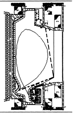
Figure 1-1 shows a cross-section of the Alcator C-mod tokamak. C-mod has a com-pact, high field torus design. C-mod typically operates at a toroidal field strength of 5-6 T and a plasma current of a little over 1MA though it is designed to be capable
of operation with a 9 T field and 3MA current [1]. The average electron density of
most shots is between 1 and 4 x 10² 0m- 3. The tokamak has a major radius of 0.67 m and a minor radius of 0.21 m (see Figure 1-1).
1.2 Plasma Radiation
This section gives some details about the most significant plasma radiation processes.
Cyclotron Radiation
Charged particles undergoing acceleration emit electromagnetic radiation. Since mag-netically confined particles orbit about field lines they are continuously accelerated
/ .1
I i .
IL1~~~~~~~~~~L4
I: /·~~~~~~i
and so are constantly emitting. The acceleration of a particle in a circular cyclotron orbit is
acyc = w2p
(1.10)
where w, is the cyclotron frequency qB/m and p is the particle gyroradius vl/wc. The
rate of energy emission from a nonrelativistic particle with acceleration a is given by
dW 2 2 (1.11)
dt 67reOc3
If we take the velocity of the confined particles perpendicular to the magnetic field confining them to be v = 2T/m then by (1.10) and (1.11) and the definition of
we, the rate of energy emisson due to a single particle is
dW
=
q
(qB)4
2T) m 2dt 67coC3 m m qB
( q4B2
37rEo (mc) 3 T
'The power density of cyclotron emissions due to a single species is obtained by
multi-plying the last expression by the particle density of that species and using its charge,
mass, and temperature. Since electrons are much less massive than any of the other
plasma particles their contribution to plasma cyclotron emission is by far the greatest even when impurities present in the plasma are taken into account.
To this point the discussion of cyclotron emissions from the plasma was much sim-plified, particularly in that it deals only with emissions at the fundamental cyclotron
frequency. Radiation is also emitted at the harmonics of the cyclotron frequency but
at considerably lower levels. Also missing from the treatment is a consideration of
how much energy emitted by the plasma particles is actually lost. The plasma is opaque to the fundamental electron cyclotron frequency and the lowest harmonics so
the rate of energy loss from the plasma due to cyclotron emissions is small, especially
compared to losses due to other radiating processes. In the operating regime of
measurements.
Bremsstrahlung
In addition to undergoing acceleration due to their orbits in a confining field the particles in a plasma are accelerated by collisions with other particles. This is called bremsstrahlung or braking radiation and it constitutes the most significant radiation
power loss process in a pure hydrogen isotope plasma.
The maximum acceleration due to a Coulomb collision between an electron and
an ion of charge Z is given by
Ze2
acoll 4romeb 2 (1.12)
where b is the impact parameter. We can make the approximation that the collision lasts for a time 2b/v with v = /3T/m. Putting (1.12) into (1.11) and multiplying
by the duration of the collision gives the energy emitted in each collison in terms of
its impact parameter and plasma parameters. Integrating over impact parameters (bearing in mind that the minimum possible impact parameter is the electron de
Broglie wavelength) gives an approximation close to the actual bremsstrahlung power value which is most accurately given by
Pbrems e6Z2Te/ 2
(1.13)
neni 6V3/273/2E3c33/ 2 (1.13)
as the equation for the power density of bremsstrahlung emissions due to collisions between electrons and Z ions.
The classical treatment above must be corrected for quantum mechanical effects by multiplying Pbrem by the Gaunt factor g. In a fusion plasma g is near unity.
Line Radiation
radiation from those impurities is usually comparable to or greater than that due to electron bremsstrahlung.
The radiated power density due to impurity species Z has the form [4]
Prad,Z = nznefz(Te).
(1.14)
The temperature dependence fz(T,), usually obtained from theoretical calculations,
is complicated and different for every species. Nevertheless, some accurate general
statements can be made about the temperature behavior of Prad. Above lkeV tem-peratures low-Z impurities do not contribute to plasma line radiation because they
no longer have electrons to produce line emissions. In a tokamak, line radiation from low-Z impurities comes from the edge where the temperature is sufficiently low.
High-Z impurities are another story, they retain some electrons through all or most of the plasma and so radiate everywhere. In addition to radiating over a broader
range of temperatures high-Z impurities have an fz(Te) that is on average an order
of magnitude greater than low-Z impurities.
1.3 The Significance of Radiation Measurements
Radiation emitted by plasma particles and not reabsorbed by the plasma represents a
loss of energy from the plasma system. The energy lost in this way is a significant part
of the loss term in the power balance equation (1.1). For this reason it is important
to observe as closely as possible the radiation emitted by the plasma.
Several diagnostics used to study fusion plasmas depend on measuring the radi-ations of that plasma. The temperature can be measured by means of the electron
cyclotron emissions of the plasma. The value of Zeff can be determined by measuring
the bremsstrahlung radiation while excluding line radiation. Spectral measurements are used to obtain the (relative) quantities of different substances in the plasma. One of the bolorneter diagnostics covered by this thesis is used to determine the total power radiated from a plasma in the ultra-violet and x-ray regions of the EM
spec-trum. The other is an array of identical bolometers used to construct radial profiles of the plasma, volume emissivity [5]. In a tokamak radiation in this range is dominated
Chapter 2
Bolometer Operation
The Alcator C-Mod tokamak is equipped with two types of bolometric detector. One type is based on the thermal response of a metal foil to impinging photons and the other is based on the photodiode behavior of a semiconductor. At present there are two diagnostics of each type used to study plasma radiation in the tokamak. For each type there is a diagnostic used to estimate plasma radiated power and another used
to obtain radial profiles of the plasma emissivity.
2.1 Detectors
2.1.1 Foil Detectors
The first type of bolometeric detector to discuss is the foil bolometer. As mentioned
above these detectors work because incoming radiation heats a small piece of metal foil (in the case of the Alcator diagnostics, gold foil)[6]. The heating of the foil is
produced primarily by photoelectric absorbtion. The foil is in thermal contact over
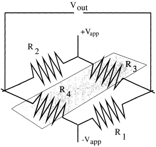
its whole surface with a thin meander resistor see (Fig.2-1) for a schematic of the meander resistor. Temperature changes in the foil are accompanied by a decrease in the resistivity of the gold resistor. A bridge circuit, shown schematically below (Fig. 2-2), is used to convert this resistivity change to a voltage signal which is amplified
Figure 2-1: Schematic diagram of two of the detector resistors.
Vout
FF
When no radiation is inicident on the bolometers, all resistances are equal to a
common value, R. The signal from the bridge circuit is then
Vout VappR= R 2 (2.1)
where Vot is the voltage measured across the circuit as shown in Figure 2-2, Vpp is
the total voltage applied to power the bridge, and AR is the change in the resistance of the exposed resistors. If we can assume that the resistance R varies linearly with with temperature T, a valid assumption for gold near room temperature, then we can write
R = AT + Rt (2.2)
with Rrt as the room temperature resistance of a single resistor element and c as the slope of the temperature-resistance relation (with units K for example) Vt is then
related to the change in foil temperature by
AT = Rrt Rrt Vt (2.3)
AT = ~ [(V_ -2) ce/2 Vpp(2.3)
'The power absorbed by the detector (as a function of time) is related to its temper-ature by
Pdet(t) = (T(t) + Tc dt (2.4)
where Tc is the cooling time and sn is a calibration constant. The relation between
Pdet and the power radiated by the plasma will be discussed in the next chapter.
The advantages of foil type bolometers are their simplicity and reliability. The bridge circuit arrangement with shielded detectors used as the reference resistors makes the elimination of signals due to background temperature changes automatic.
The detectors can be calibrated in place (see below) and do not need to be adjusted
once installed. Detector sensitivity is only slightly susceptible to neutron
bombard-rnent. Additionally foil detectors have no spectral resolution. The gold foil bolometers used on C-mod measure all radiation in their range of sensitivity. One important
con-sequence of this feature is that identifying the source of the measured radiation is not possible with any certainty using just bolometer information.
There are two main disadvantages to using foil type bolometer detectors. The
first is that; the foil is heated by neutral particles as well as by EM radiation. There is therefore no way to distinguish between these two channels of plasma energy loss using foil bolometers alone. The second drawback is that foil bolometers are slow.
The value of Tc, the cooling time has a lower limit which in turn limits the time resolution of the diagnostic.
2.1.2 AXUV(Diode) Detectors
A photodiode allows more or less current to pass depending on how much light is incident on it. The photodiodes used as bolometric detectors on C-Mod are sensitive to light in the soft x-ray to ultraviolet range responding best from 20eV to 10keV [7].
Advantages of the diode detectors over the foil detectors are their faster time re-sponse, their insusceptibility to heating by neutrals, and a simpler circuit to tune. The major problem with using these detectors is that their spectral response is less certain than for foil bolometers and the absolute calibration is known to vary depend-ing on environment. This type of detector is especially susceptible to acquirdepend-ing thin coatings of material in the course of tokamak conditioning which play havoc with the
calibrations.
2.2 Arrangement
2.2.1 Detector Arrays
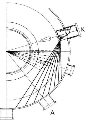
Both of the bolometer arrays (foil and diode) used to obtain plasma emissivity profiles
are contained in a box mounted at K-Port on C-Mod (see Fig. 2-3). The box is at
about the midplane and the apertures face A-port. Each array consists of sixteen viewing chords which span the minor radius of the tokamak.
K
Figure 2-3: Bolometer Box Arrangement. Solid lines: Sample viewing chords; Broken
Figure 2-4: 27r Bolometer View; Solid lines: Theoretical; Broken lines: With limiters and tiles in place.
2.2.2
2v Detectors
The 27r foil and diode detectors are both located outside the plasma and considerably below the midplane. Figure 2-4 shows that these detectors admit light from an entire cross-section of the confined plasma, but exclude the divertor region.
2.3 Calibration of Foil Bolometers
2.3.1 Electronics
All the detector amplifiers have to be periodically adjusted to minimize voltage
base-line offsets, though small offsets are removed when the data is analyzed. The foil
ItOOpF
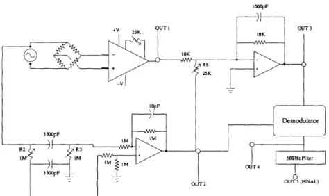
Figure 2-5: Simplified circuit diagram
Figure 2-5 is a simplified circuit diagram for a single foil bolometer channel. The
main parts of the circuit are the detector itself, the instrument amplifier, a phase shifter, a nulling circuit, and a (synchronous) demodulator. When calibrating/tuning the bolometer electronics typically only the variable resistors labeled R2, R3, and R8
on the circuit diagram are adjusted. Note that all of the IC components are powered at 12V.
Amplifier
The instrument amp is mostly for adjusting the offset of the detector signal. However
the 10kQ range variable resistor has to be changed only occaisionally. The offset signal coming from the detector channel (OUT 1 in the figure) is fed into an oscilloscope for
use in later calibration steps.
Phase Shifter
To properly demodulate the detector signal we need a signal that is 180 degrees
out of phase with the 5kHz driving signal. The phase shifter portion of our circuit provides this signal but it must be tuned from time to time. To accomplish this the output of the phase shifter (OUT2) is plotted on the other channel of an oscilloscope
half-period phase difference between the two plotted circuit outputs is achieved.
Nulling Circuit
We want to remove as much of the driving signal as possible so we use a nulling circuit
(we combine the out-of-phase signals through an op-amp). We want the minimum output (OUT 3) possible from this part of the circuit. The resistor R8 is adjusted
to change how much of the phase-shifted signal is added. Since the adjustments to
the phase shifter resistors R2 and R3 is done by eye it is usuall necessary to use the output of the nulling circuit to more finely tune the phase shifter to obtain a minimum
signal.
Final Steps
The output; of the Nulling circuit is synchronously demodulated using the output of the phase shifter as the synchronizing signal. The output of the demodulator is
then put through a 500Hz low pass filter (7-pole Bessel) and sent on to the recording
electronics. The demodulator (OUT 4) and filter (OUT 5) outputs are checked to
make sure nothing goes wrong in those steps.
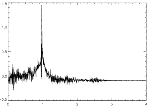
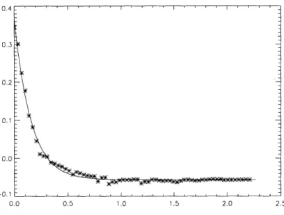
2.3.2 Time Constant
The time constant for each channel is determined by finding a shot that ends in a
disruption and fitting an exponential curve to the end of the raw voltage signal from
the detector bridge. An example of such a fit is shown in Figure 2-6 The decay
constant of the exponential will be the reciprocal of the channel's cooling time. The
cooling time constants of the channels vary between 0.08 and 0.15 seconds.
2.3.3 Sensitivity
The sensitivity of the detector is just a measure of how a measurable quantity, such
ra-0.4 0.3 0.2 0.1 0.0 -0.1 0.0 0.5 1.0 1.5 2.0 2.5
Figure 2-6: Fitting a disruption curve to obtain c
calibration constant is a measure of sensitivity. First we consider the sensitivity of the bolometer in a "cold" state. That is, the sensitivity of the bolometer to a single
power source absent any other power in the bridge. To do this we simply compare the resistance of the detector when no voltage is applied to its resistance when a known
voltage is applied and a known power is dissipated in the foil.
The procedure is to (1) measure the resistance (R) across a detection resistor with the power to the electronics rack turned off, (2) power the electronics and apply
a DC voltage of .5V to the bridge, (3) balance the calibration bridge by adjusting the resistance of one leg so that the voltage across the bridge(Vbr)is zero,(4) apply
5V(= Vapp) to the bridge and measure the new voltage across the bridge (no longer
zero). This procedure is applied to each detector channel. The "cold" sensitivity of
the channel defined as
Sd Vbr 1 Vbr R (2.5)
Vapp/2P Vapp/2 (Vapp/2)2
where R is the resistance of one of the detector legs of the bridge, consisting of just one resistor. When the bolometer is in use, the "cold" condition does not
hold - in operation each bolometer detector is an AC bridge circuit with a 5Vpp
temperature of the resistors and hence the measured signal. Fortunately, if we know
how the detector resistance depends on temperature (or incident power from any
source) we can relate the sensitivity at one temperature (such as when the detector is "cold") to the sensitivity at any other temperature.
We can begin with a definition of the sensitivity (S) of the foil bolometer
S-dP R (2.6)
Where R is the resistance of the bolometer element and P is the power incident on the bolometer, either due to radiation or current running through the bridge. If we assume that R varies linearly with P then we can write
dR
R = Ro + d P (2.7)
dP
with a constant. The power dissipated in the bolometer is given in terms of the voltage in the resistor by
V2
P
=
R--
(2.8)
and we can use this expression for the power with the linear equation for resistance
to obtain the following quadratic equation for the resistance
R2- RoR- dRV 2 = 0 (2.9)
dP
which has as its solution
R+ Ro + 4 -dV 2 /2. (2.10)
We can see from the definition of S that if we can assume that dR is constant then
the ratio between the sensitivities at two different temperatures is the reciprocal of the ratio of the bolometer resistances at those temperatures
S2 _ R1 (2.11)
S1 R2
so our solution for R can be used to relate the sensitivity of a bolometer when it is
cold to the sensitivity when it has AC current passed through it during operation.
Since we do not necessarily know d and we do know Scold it is useful to invert
(2.6) at S = Scold to get the constant slope. Using this information and taking (2.11) can be rewritten
Swarm
= cold
_a) + [(1 -a)
2+ b]2)
{(1 - a) ± [(1 - a)2 ± b]2( where a =- Scold 2and b = ScoldV 2en and a factor of RO was taken out after Ro was
4Rold Rcold
expressed in terms of Rcold with Vapp taken to not be negligible for that purpose.
2.4 Determining the Position of AXUV Tangency
Radii
2.4.1 Setup and Procedure
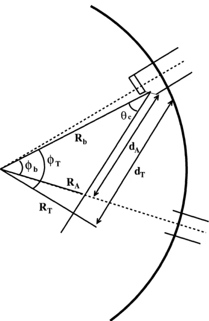
In order to interpret measurements made with bolometers we must, for each detector channel, know the radial position at which the viewing chord corresponding to the de-tector intersects with a radius of the tokamak at right angles. This is called the radius of tangency of the detector. This radius is not measured directly. The information we have available to determine it is the radial and angular position of the focus of the viewing chords (at the aperture of the AXUV detector) and, for each channel, the radial location of the intersection of the viewing chord with a radius of known toroidal
angle. This last value, labeled RA, is found by placing a small mercury vapor lamp
in the tokamak and measuring its distance (in the A-port plane) from the inner wall 'when the AXUV detector channel of interest has its maximal response. The known distance to the inner wall is added to the measured distance to give RA The knowns
Rb = radial location of the aperture
Ob = angle between the aperture and the center of A-port
RA = radial location of intersection between the channel viewing chord and the
tokamak radius passing through the center of A-port
dA = the distance along the viewing chord between the aperture and RA
0c = Angle between the radius intersecting the aperture and the channel viewing
chord
OT = Toroidal angle between Rb and the tangency radius
dT= The distance along the viewing chord between the aperture and the tangency
radius
RT = The radial coordinate of the tangency point that we seek
2.4.2 Calculation
To calculate the tangency radius we need to apply some trigonmetry. We recall the Law of Cosines for a triangle with sides a, b, c opposite angles A, B, C respectively:
c2 = a2 + b2 _ abcosC (2.13)
which can be applied to the triangle with sides a Rb, b - RA, C - dA(so C - b)
to obtain the length dA. Having dA we can apply (2.13) a second time, but with
a - Rb, b - dA, c - RA(so C Oc) and rearrange to get
2cos RbdA
Now since the triangle with sides RT, Rb, dT is a right triangle we have
dT = Rbcos O RT = Rbsin c
OT = 2 Oc
RT
Figure 2-7: Schematic for the determination of tangency radii.
5 I 4 4 I
which are the values we wanted.
2.4.3 Results
The critical parameter obtained from these calculations is the value of RT for each channel. The results are shown in Table 2.1 along with values of RT obtained from various sources for comparison (all values are in millimeters).
The values in the columns labeled 1999 and 2000 are values reported by Dr. Boivin
for measurements made in the '99 and '00 run campaigns(note that my convention for ordering channels is the opposite of his). It is not possible to associate the radii obtained from the design drawing for the AXUV bolometers to particular channels. However, the first and last measurements from the drawing match well with the first and last channels calculated from our most recent measurements. I have listed the
drawing measurements in the row of the channel for which they are closest to our
RT values but that correspondence should
marked with "*" are broken. These results
not be taken too seriously. The channels show that the variation of these
measure-Table 2.1: Tangency Radii for Ch 2002
]
1999J
2000 | Drawing] 1 921.9 920.6 898.8 920 2 916.2 914.4 893.3 3 * 906.8 886.5 904 4 900.2 897.6 878.0 5 892.2 887.6 869.1 880 6 * 875.5 858.1 7 866.8 861.9 845.6 8 855.6 846.7 831.6 852 9 834.9 829.8 815.9 10 821.4 811.3 798.7 820 11 802.1 791.1 779.7 12 781.4 769.2 759.0 776 13 759.5 745.9 736.9 14 736.4 721.2 713.4 728 15 712.4 695.1 688.4 16 681.1 668.0 662.4 672 AXUVments from setup to setup is well within the range of accuracy of the reconstructions. These measurements can therefore be trusted and used in interpreting the AXUV data.
The AXUV tangency radii are also useful for generating tangency radii for the
core foil array. Since each of the four blocks of foil detectors are mounted at a known
angle to the AXUV plate and the locations of the detectors on the blocks are fixed, we
know the angles between all of the foil viewing chords and any of the diode viewing chords. With these angles and a measured RA from one of the diode channels we get
the RA values for the foil detectors and can repeat the process described above to get their tangency radii.
Chapter 3
Spatial Radiation Profiles
3.1 Inversion Problem and Solution
The problem faced when using bolometer data to generate spatial profiles of the
plasma emissivity is one of converting a line integrated power density to a volume
emissivity [9]. The mathematical technique for recovering spatial information from
line integrated data is often referred to as Abel inversion. Problems of this kind are
common to the inversion of data from other plasma diagnostics and astrophysical
observations so the basic technique is well developed.
3.1.1 Circumstances and Assumptions
The tokamak is circularly symmetric so the bolometer views, that is the lines of the
integration are all chords. We will assume the plasma is toroidally symmetric so that the viewing chords can be treated as intersecting their corresponding tangency radii at the same toroidal angle. This means we also assume the radial emissivity profile
we obtain is applicable all around the tokamak. Figure (3-1) shows the situation for
Figure 3-1: Diagram for a single viewing chord, bordered by dashed lines. (After-Bockasten 1961 [10])
3.1.2 Inversion
If we define e(r) to be the volume emissivity in units of power per unit volume then
the line integrated emissivity or brightness (in units of power per unit area) for the
detector channel, which we will hereafter identify by its tangency radius (y in Figure (3-1)), is given by
b(y) = 2 e(r)dx. (3.1)
Since triangle xyr is a right triangle x = v/r-y, we can change equation(3.1) to an
integral with respect to the coordinate of interest r.
'ro 1
b(y) = 2 e(r)(r2 - y2)- rdr (3.2)
Now we can use Abel's inversion to write
e (r)o
db(y2 r2)ydy (3.3) 7 r dyFigure 3-2: Diagram for a single chord. (Bockasten 1960)
db in this equation is known because we have several channels in the bolometer array.
The continous variable equations discussed in this section cannot be applied directly to our bolometer data because we have a limited and discrete set of power measurements
each of which may contribute differently to the complete profile.
3.1.3 Calculation
The actual calculation of the spatial emissivity profile is carried out using matrix
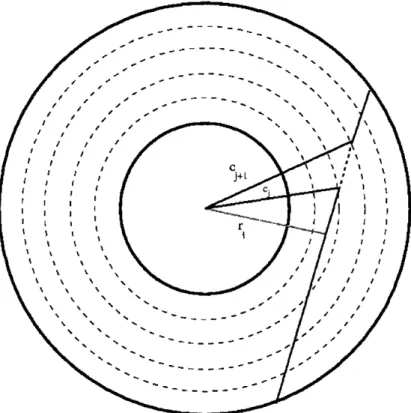
methods. We begin the finite treatment of the inversion problem by defining a series of concentric circles separated by equal increments in radius as shown in Figure (3-2).
We identify the j-th circle by its radius cj. These radii constitute a set of radial coordinates onto which the inversion is mapped, corresponding to the coordinate r in the previous section. We can also label the tangency radius of the viewing chord of the ith detector by its length ri. This is a discretization of the coordinate y in the
adjacent circles cj and cj+l is
= 2( Cj -r-
)
- (3.4)Figure (3-2) illustrates this. The factor of two is again present because equal portions
of the viewing chord lie between the circles on both sides of the tangency radius. The
rows of the matrix S are thus sets of discrete x coordinates and each row corresponds to a particular detector view. S is what relates the tangency radii of the detectors to our discrete coordinates.
Now that we have discretized versions of the various coordinates of the
previ-ous section we can rewrite the integrals found there as matrix products
(matri-ces will be denoted by capital letters while lower case symbols stand for vectors).
Equation(3. 1)then becomes
b(cl) = Slke(rk) (3.5)
k
Finding the emissivity vector e is now a matter of inverting (3.5) subject to two conditions(the following comes from [11]). First, we want to have a minimal (Se -b) 2
so that we obtain the least-squares solution to our problem. Secondly, we wish to ensure the smoothness of E. We do this by adding a term proportional to the square
of the second derivative of e, (De)2, to the quantity we seek to minimize. Therefore,
we want to minimize
K = (Se - b)2+ E(De)2 (3.6)
where D is the discrete second derivative matrix given by
Di,i = -2
Di,i- = 1
Di,i+l = 1,
minimum is found by solving
O = [(eTST - bT)(Se - b) + eTDTDe]
de de
= 2STSe + 2EDTDe - 2STb
The solution is then given by
(STS + eD D)e = STb (3.7)
Now let's define a matrix M as follows to simplify the expression of the final inversion
M = STS + EDTD (3.8)
A singular value decomposition is carried out numerically to obtain a diagonal matrix
W such that
M = UWV (3.9)
with W a diagonal matrix and U and V mutually orthogonal. The pseudo-inverse matrix used to obtain the solution to the matrix equation is then
M-1 = VW-1UT (3.10)
where W -1 is the same as W with the nonzero values (the singular values) replaced
by their reciprocals. Finally, the emissivity is just
e = M-STb (3.11)
where e is a vector of volume emissivities at the radial data points at the recorded
times and b is a vector of line intergrated emissivity or brightness readings from each
1.5 1.0 0.5 0.0 -0.5 C'I 1 2 3 4
Figure 3-3: The signal from a single channel.
It is easiest to see from the matrix form of the calculation that to obtain the emissivity at some radius we add up the powers absorbed by the detectors with the
contribution of each weighted by how much of the detector's viewing chord is in the
region corresponding to the radius of interest.
The raw output of a single detector channel typically looks like Figure (3-3). This raw signal (Vs) is related to the power absorbed by the detector channel Pabs by the
equation
Pabs = ( + dV) 1 (3.12)
dt V))V S
where Vi, is the input voltage amplitude across the detector bridge and Tc and S
are the quantities calculated as part of the calibration of the detector (see Chapter 2). This P,s absorbed by a detector channel is proportional to the radiated power absorbed by a unit of area facing the plasma directly because the measured voltage is, as discussed in Chapter 2, proportional to the temperature change in the detector. The radiated power absorbed by the detector is given by.
Et in this expression is the etendue of the detector channel, given by
ApAd
Et = 12 (3.14)
where Aap is the area of the aperture in the bolometer box,Ad is the effective aperture
due to the size of the bolometer detector foil and 1 is the distance between. We can see that dividing Pabs by Et gives the correct units for b.
As can be seen from Figure (3-3) the measured voltage signal V, is quite noisy. Taking the derivative of the signal, as is necessary to obtain Pabs magnifies the noise so that simple, local average smoothing is not enough to suppress it. The noise filtering
technique used for the Alcator foil bolometer array data is a procedure called Lee
filtering which makes use of the local statistics of the measured signal. The filtering algorithm was developed for use in suppressing speckle noise in satellite images [12]. The equation for the filtered signal y in terms of the measured signal z is
var(y)
+Y Y± + var(y) (3.15)
where
var(y) = var(z) + 2 (3.16)
and var(z) = z/(n - 1) and all averages are taken over 2n - 1 data points. The smoothing is applied both to the measured voltage and its derivative but the
smooth-ing must be carried out over a larger time window (about twice as large) for the derivative. For the C-mod foil bolometer array the time window is 40 milliseconds. The effect of the filtering procedure can be seen by comparing Figure (3-3) to Figure (3-4).
Following this procedure for each detector channel we can obtain a brightness profile like the one shown below in Figure (3-5). The brightnesses from the different chords can now be inverted as described above, following Equation (3.11) to give the volume emissivity profile we are after which is shown here.
1 2 3
Figure 3-4: The Lee filtered signal from a single channel.
0.80 0.85 0.90
Major Radius (m)
Figure 3-5: Brightness Profile 0.8 0.6 0.4 0.2 0.0 -n ? 0) , , , I I , , , ,I , I , , I , , I I I 4 0.6 0.5 N 0.4 3: ¢ 0.3 c m 0.2 0.1 0.0 0.75 0.95
...I...
...I.-I...-I.-.1.0 0.8 In W 0.6 0.4 E 0.2 0.0 0.75 0.80 0.85 0.90 0.95 Major Radius (m)
Figure 3-6: Emissivity Profile
3.2 Sources of Error
There are two main sources of error in the radiation profile as measured by the foil
bolometer array: the voltage offset and the noise in the detector and associated
electronics.
3.2.1 Detector Voltage Offset
In addition to varying from channel to channel as one would expect the voltage offset
of the various channels also varies from shot to shot and linearly within shots (see
Figure (3-7)). We try to remove this offset as the data is analyzed by subtracting a linear fit to the averages of the first few and last few time points where no real data is taken. We denote regions where no data is available from the plasma with negative
times. Unfortunately, there is still uncertainty in the calculation of the magnitude of
the offset which must be included in the error.
3.2.2 Detector Noise
-0.10 -0.05 0.00 0.05 0.10 Time(sec)
Figure 3-7: No marking: Signal; Stars: Signal with approximate offset subtracted.
the errors of the line integrated powers are about 15%. These errors have different effects depending on the channel they occur in as discussed in the next section.
3.3 Error Sensitivity
'The errors in the line integrated data must be propagated through the inversion
process to give proper error estimates in the final profile.
3.3.1 Relative Sensitivity of the Channels
It turns out that error accumulates as one probes deeper into the plasma [13] and the accuracy of profile data is more susceptible to errors in the signals from the
innermost viewing chords of the bolometers. Figure (3-8) shows that at the same fractional error in input signals the inner viewing channels have much larger errors.
Notice how insignificant the error due to the outermost channel is compared to the nearly 50% error resulting from the same detector error in the innermost channels. The next two figures show the result of this high sensitivity of the inner channels for
the final profiles.
Figures (3-9) and (3-10) illustrate the the significant differences in the effect of A V o c cr v,
mi .5 E Ld 0.80 0.85 0.90 0.95 Major Radius (m)
5x1 05 4x10⁵ 3x 05 2x105 lx105 0 0.75 0.80 0.85 0.90 0.95
Figure 3-9: Outer Channels: Errors of 10,15, and 20%
I":;i \· \ i b r \\`\ , 1 · ': i'll :In :il I · I : ·/ c? - I I I I 1 I I I I I I . , I\ i ,\I, .ii - - - c . - . . - . . . . - r 1~~~~~~~~~~~~' I I
5x 05 4x10⁵ 3x '105 2x 05 1 x10⁵ 0 0.75 0.80 0.85 0.90 0.95
errors on inner channels compared to errors on outer channels. In Figure (3-9) we
see that errors in outer channels do not have a strong effect on the overall shape of the profile. In contrast, Figure (3-10) shows the drastic effects of similar errors on emissivity profile shape when the errors occur in a channel just ten centimeters closer to the plasma core. Hopefully, these examples have demonstrated the nature of error propagation in an Abel inversion.
The emissivity profiles discussed here can be used to recover the plasma radiation as it is measured by the 27r bolometers. The radiated power absorbed by the 27r foil is given by an expression like (3.12). An approximation (which assumes poloidal and
toroidal uniformity of radiation) for the power radiated in the detectable range is
then given by
P2 = Pabs,27r Awar (3.17)
A27rdet
where A2,det is the area of the 27r detector foil and Awall is the inner surface area of
the tokamak. A reconstruction from the array data can serve both to provide new information about the plasma and as a check of our calibrations and calculations. Comparisons of this kind are discussed in the next chapter.
Chapter 4
Some Results
4.1
Overview
The results to be discussed in this thesis are of two categories: measurements of
plasma radiated power and measurements of the plasma emissivity profile. As men-tioned at the end of the previous chapter radiated power measurements can be ob-tained both from the bolometer arrays used to generate emissivity profiles and the 27r foil and diode bolometers. Results of this kind help us to determine how much energy is being lost from the plasma via radiation under various conditions. In this
chapter one thing we will examine is how good the different bolometers are at provid-ing a measurement of this radiation as well as the conditions under which it differs significantly (e.g. when impurity concentrations are high). Emissivity profiles gath-ered using the bolometer arrays tell us where in the plasma the radiation is chiefly coming from. We use this information on the local emissivity values together with
information about local plasma properties obtained with other diagnostics to try to identify the main sources of radiation in the plasma. Examples of this kind of work
which will be discussed in this chapter include using temperature profiles with the emissivity profiles and known temperature-line emission curves of different species to identify the main radiating species and determining the effect of the presence of a
2.0 1.5 3 o 1.0 .o QY 0.5 0.0 0.1 0.2 0.3 0.4 0.5 0.6 0.7 0.8 Time(seconds)
Figure 4-1: Foil Array Radiated Power
4.2 One-Hundred Percent Radiated Power
When the plasma has a high impurity content we expect that all of the power input will be radiated away. Under these conditions we can try to calibrate the bolometer diagnostics (in fact there are not many other practical options for calibrating the diode bolometers). Figure (4-1) shows the radiated power trace for a shot with impurity injection. The time of the last impurity injection (which brings the impurity
concentration up to its final value before disruption) is shown as a vertical line on the
trace.
The next Figure (4-2) shows the time traces of the radiated power obtained from the foil array and the two pi foil bolometer, along with the plasma current and average density which are important in determining the radiated power, for the same shot.
The fraction of the total input power radiated for the same shot is shown in
Figure (4-3) for the segment of time following the final impurity injection. As shown
in Figure (4-3) the bolometer array measures 100% radiated power fraction for this shot (accurate to about 5%) before disruption, as expected. For the plasma shown the power input was entirely ohmic and the impurity injected was argon. Similar results were obtained with a neon injection.
To determine the validity of this result the radiated power fraction as measured by
I . ... 11 ... ,, I,,.,,., , 1,-.,.1. I,,,, .,, 1l.1 -,, * 1 .* 1 . .1 .. I [ . . . .. . I .' ' .. . . I " ' ' ' ' ' ' '
-0.8__
E 0.7
0.61 0.2 0.3 0.4 0.5 0.6 0.7 08
0.1 0.2 03 o14 &. o16 o17 .
1 A l l l l l l I~~~~~~~~~~~~~~~~~~~~~~~~~~~~~~~~~~~~~~~~~~~~~~~~~~~~~~~~~~~~~~~~~~~~~~~~~~~~~~~~~~~~~~~~~~~~~~~~~~~~~~~~~~~~~~~~~~~~~~~~~~~~~~~~~~~~~~~~~~~~~~~ 2 1 II II 0.1 0.2 0.3 0.4 0.5 Time(seconds) 0.6 0.7 0.8
Figure 4-2: Plasma Properties and Radiated Powers
1.2 1. 0. 0. 0. 0. 0 0 8 6 .4 .2 .0 0.72 0.74 0.76 Time 0.78 0.80
Figure 4-3: Radiated Power Fractions for the Foil Array (solid) and 27r (dashed) Bolometers R E o c5 c· la L v Z r -N Ol"I I 0.1 0.2 0.3 0.4 0.5 0.6 0.7 0.8 0.1 0.2 0.3 0.4 0.5 0.6 0.7 0.8 0.1 0.2 0.3 0.4 0.5 0.6 0.7 0.8 0.1 0.2 0.3 0.4 0.5 0.6 0.7 0.8 , , I , , , I , I II.... -J . .. .. ... I 2 . . . -- I I I I I I I , . . . r I I I~---1 U --1 C o o L i,
6 o 4 c) C-O (, a-C 2 Q) L 0 Distribution of Powerfraction 0.70 0.80 0.90 1.00 1.10 1.20 Array Fraction
Figure 4-4: Array Prad Fraction Histogram
Toroidal Field 5.4 T Average ne 1.5 1020m-3
Average Te 1.5 keV Average Ip .78 MA
Table 4.1: Parameters for Figures 4-4 and 4-5
both the foil array and the 2 foil detector were determined at multiple time points on several shots with maximum radiated power. The results are shown in histogram
form in Figures (4-4:Array) and (4-5:2w).
For shots for which 100% radiation is expected the radiated power fraction
recon-structed from the foil array bolometer data averages 98% with a standard deviation
of about 10%o and a range of +/-20%. The values obtained from the 2r foil for the same shots average 100% with a 16% deviation and a +/-20% range.Table 4.1 shows
8 6 C) () o );y , LL-2 0 Distribution of Powerfraction 0.90 0.95 1.00 1.05 1.10 1.15 1.20 2 Pi Fraction
Figure 4-5: 27r Prad Fraction Histogram
4.2.1
Effect of RF Input on Power Fraction
In this section we will cover the attempt to determine what changes in radiated power fraction, if any, result from increasing the input of RF heating power to the plasma.
We will also study the effect of the plasma mode on the way radiated power responds to total input power. The results shown in Figure (4-6) were obtained by averaging
the radiated power fraction data from several instances with the desired input RF power. Data from both foil array reconstruction and the 2r foil bolometer are plotted. Figure (4-7) is similar to Figure (4-6) except that in this case the radiated power output is plotted against the input power due to both ohmic and radio frequency heating.
Table 4.2 shows the average plasma conditions (prior to RF input) of the plasmas
from which the power data for the figures was taken.
4.2.2 Discussion
0.0 0.5 1.0 1.5 2.0 2.5 RF Input Power (MW)
Figure 4-6: Radiated Power Fraction vs. Input RF Power 3.0
1 2 3 4
Input Power (MW)
Figure 4-7: Radiated Power Fraction vs. Input Power
For Figures 4-6 and 4-7; No Marking: Foil 2r (H-mode), Stars: Foil Array (H-mode), Diamonds: Foil 2r (L-mode), Squares: Foil Array (L-mode).
0.7 0.6 0.5 0.4 0.3 0.2 0.1 0.0 C O -o Ll-.S) T3 C) Qo 2.0 1.5 0 0a w 1.0 0o 0.5 0.0 0
Toroidal Field 5.4 T
Average ne .9 102 0m- 3 Average Te 1.5 keV Average Ip .79 MA
Table 4.2: Parameters for Figures 4-6 and 4-7
also see that the plasma radiates more when in mode than when in L-mode. H-mode is a high confinement H-mode in which a transport barrier develops in the plasma
edge leading to an increase in the plasma density and a doubling (approximately) of the confinement time. The actual ratio of the energy confinement time after the transition to H-mode to the confinement time before is called the H factor. One
feature of H-modes which is significant for our discussion is that they do not occur below a threshold input power (see more about H-modes in e.g. [3]. Figure (4-7)
shows that data from shots that at some point have an H-mode match the data from
shots that remain in L-mode for their duration when input energies are too low to produce an H-mode. Figure (4-7) also give us a better handle on the difference in radiated power between H-mode and L-mode plasmas. We can see that in both cases the radiated power scales linearly with input power. The difference is that in H-mode
the plasma the radiated power rises with input power about three and a half times
as fast as in the L-mode case. The reason for the power difference would not be so clear from Figure (4-6) alone.
1.0 0.8 r-, 0.6 ... 0.2 0.0 0.82 0.84 0.86 0.88 0.90 0.92 Major Radius (m)
Figure 4-8: Standard Shot Emissivity Profile
Toroidal Field 5.4 T
Average ne .9 102 0m-3 Average Te 1.5 keV Average Ip .79 MA
Table 4.3: Parameters For Figure 4-8
4.3 Emissivity Profiles
Typical emissivity profiles for unmodified, ohmically heated plasmas in Alcator C-mod look like the one shown in Figure (4-8).
The main, consistently reproduced features in deuterium plasmas without inten-tional injection of impurities are a strong peak at R=0.85 m and a minimum at R= 0.87 -.89 m. Emissivity values at the minimum are usually about a tenth the mag-nitude of the maximum emissivity. Sometimes the reconstruction of the emissivity profiles returns negative emissivity values. This is an unphysical result and must be accounted for. The problem arises because the reconstruction of the emissivity profile assumes a plasma that is always everywhere transparent to the radiation of interest, and this is not the case for the real plasma. The general properties of shots like this

![Figure 3-1: Diagram for a single viewing chord, bordered by dashed lines. (After- (After-Bockasten 1961 [10])](https://thumb-eu.123doks.com/thumbv2/123doknet/14179249.475927/36.918.247.663.126.525/figure-diagram-single-viewing-bordered-dashed-after-bockasten.webp)