Analysis of word-order universals using Bayesian phylogenetic inference

(1)

Analysis of Word-order Universals Using Bayesian

Phylogenetic Inference

ARC'VES

by

Pangus Ho

S.B. Computer Science and S.B. Physics, M.I.T., 2011

Submitted to the Department of Electrical Engineering and Computer Science in Partial Fulfillment of the Requirements for the Degree of

Master of Engineering in Electrical Engineering and Computer Science at the Massachusetts Institute of Technology

May 2012

The author hereby grants to M.I.T. permission to reproduce and to distribute publicly paper and electronic copies of this thesis document in

whole and in part in any medium now known or hereafter created.

Author:

bepartment of Electrical Engineering and Computer Science May 18,2012

Y20)

KTh

Certified by:

/

Accepted by:

/

Prof. Robert C. Berwick

Thesis Supervisor

Prof. Dennis M. Freeman Chairman, Masters of Engineering Thesis Committee

(2)

(3)

Analysis of Word-order Universals Using Bayesian Phylogenetic Inference by

Pangus Ho

Submitted to the

Department of Electrical Engineering and Computer Science May 18, 2012

In Partial Fulfillment of the Requirements for the Degree of Master of Engineering in Electrical Engineering and Computer Science

ABSTRACT

This thesis examines the novel approach by Dunn et al. (2011) that employs the Bayesian phylogenetic inference to compute the Bayes Factors that determine whether the evolutions of a set of word-order traits in four language families are correlated or independent. In the first part of the thesis, the phylogenetic trees of the Indo-European and Bantu language families are reconstructed using several methods and the differences among the resulting trees are analyzed. In the second part of the thesis, the trees are used to conduct various modifications to the original experiments by Dunn et al. in order to evaluate the accuracy and the utility of the method. We discovered that the Bayes Factors computation using the harmonic mean estimator is very unstable, and that many of the results reported by Dunn et al. are irreproducible. We also found that the computation is very sensitive to the accuracy of the data because a one-digit error can alter the Bayes Factors significantly. Furthermore, through an examination of the source code of BayesTraits, the software package that were used compute the Bayes Factors, we discovered that Dunn et al. supplied invalid inputs to the software, which renders their whole calculations erroneous. We show how the results of the computations would change if the inputs were corrected.

Thesis Supervisor: Robert C. Berwick

(4)

(5)

Acknowledgments

I would like to express my greatest gratitude to my thesis supervisor, Prof. Robert C.

Berwick, for his invaluable help and tireless mentorship. He has been thoroughly involved in the planning, the design, the execution, and the analysis stages of the thesis. He taught me skepticism and critical thinking. He suggested brilliant ideas whenever I was completely lost. He helped me run the computationally intensive tasks on his machines. Without all his assistance and guidance, this thesis would not have been possible.

I further want to thank Prof John Guttag, Prof Eric Grimson, and Prof. Srini Devadas,

for employing me as a teaching assistant for the M.I.T. class 6.00, "Introduction to Computer Science and Programming," for two semesters. The teaching experience has made my year much more colorful and worthwhile.

Finally, I would like to thank my parents, my siblings, and my friends for their relentless support and encouragement.

(6)

(7)

Introduction

The question of word-order universals has been a topic of considerable interest since it was first studied by Greenberg (1963). Greenberg analyzed the structure of many different languages and found indications of implicational relationships. For example, he noted that languages where the verb comes at the end of a sentence, as in German or Japanese, would also tend to have postpositional phrases rather than prepositional phrases. The correlation is clearly not perfect, since, for instance, German is verb final but has prepositional phrases.

While controversy thus remains regarding the origins and nature of word-order correlations like this, one new way of analyzing this data has been put forward by Dunn, et al. (2011), in the context of a Bayesian phylogenetic analysis coupled to a stochastic models of how correlated 'traits' like verb-final and postpositional order might evolve over time. The method, originally developed to describe correlations with more purely biological traits like a genetic measure coupled with an external behavior, Dunn et al. applied the method to a large set of linguistic data. With this method, he discovered that while the evolutions of many pairs of word order traits appear to be correlated, the dependencies are not general but specific to certain language families. The purpose of

(10)

this thesis is to analyze their findings with an eye towards evaluating the accuracy and utility of this method, pushing the proposed model by applying sensitivity analysis to their model.

The theoretical background and past work around this topic will be presented in this chapter. In Chapter 2, the linguistic phylogenetic trees that were published by Dunn et al. are reproduced and investigated. In Chapter 3, we explore various ways to modify the original Bayesian analysis by Dunn et al. in order to test the robustness of the approach. Conclusions and future work are discussed in Chapter 4.

1.1 Word-order Universals

Based on the study of the grammars of approximately 30 languages, Greenberg (1963) formulated a list containing 45 generalizations, known as the Greenberg's linguistic

universals, which include claims that certain syntactic and morphological features of

languages are correlated. The universals are commonly referred to by the number; for example, linguistic universal #4 is that "with overwhelmingly greater than chance frequency, languages with normal SOV order are postpositional."

One of the important expansions of the original study by Greenberg was the 1992 paper

by Dryer, which analyzed 625 related and unrelated languages worldwide to determine

(11)

Among others, Dryer discovered that the languages with dominant verb-object ordering (i.e. where verbs precede the objects) tend to have verb-subject, adposition-noun (prepositions), noun-genitive, noun-relative clause orderings, where the languages with dominant object-verb ordering (i.e. where verbs follow the objects) tend to have the opposite. Dryer also claimed that the adjective-noun and demonstrative-noun orders do not correlate strongly with the verb-object order. Furthermore, he proposed that the correlation may result from the tendency of a language to be consistently left-branching or right-branching in its syntactic trees.

Dunn et al. (2011) readdressed the issue by applying computational phylogenetic methods to examine the universality of those so-called language universals. They analyzed the correlation among eight word-order traits, which for conciseness will be referred to by their three-letter abbreviations:

e ADJ: adjective-noun order e ADP: adposition-noun order

e DEM: demonstrative-noun order e GEN: genitive-noun order

e NUM: numeral-noun order - OBV: object-verb order

e REL: relative clause-noun order

(12)

The word-order data that they used were collected from the World atlas of language

structures (Haspelmath 2008), and encompass 79 Indo-European languages, 130

Austronesian languages, 66 Bantu languages, and 26 Uto-Aztecan languages. They subsequently used Bayesian analysis to determine whether each of the word-order traits co-vary with the other traits along the evolutionary lineages of the languages.

The Bayesian phylogenetic approach in general will be described in Sections 1.2 and 1.3, while Dunn et al.'s results, along with the controversies surrounding it, will be

summarized in Section 1.4.

1.2 Bayesian Phylogenetic Analysis

Bayesian phylogenetic analysis is a method to infer the posterior likelihood distribution of a model of evolution, given the traits data and a set of phylogenetic trees. The method is widely used in computational biology, for example to determine whether the mating system and the advertisement of estrus by females have evolved together or independently in primates (Pagel & Meade 2006). Dunn et al. employed the same method to infer whether or not two word-order traits have co-evolved.

The basis of the analysis is the Bayesian inference, which can be summarized as follows. Suppose that we have a set of observations 0 with probability P(O). In biology, the observations are typically in the form of a molecular sequence alignment; in the work of

(13)

Dunn et al., the observations are the word-order traits. The evolutionary model, for

simplicity, is specified with a vector of model parameters, V. If one wants to build

phylogenetic trees for instance, then V would encode the tree structure and the branch

lengths. We want to compute the posterior probability distribution of the model, P(FJO), which is the likelihood distribution of the model parameters given the observations. This

can be computed if we know the prior probability distribution of the model, P(V), and

the conditional probability distribution of the observations given the model parameters, P(OI V), by using the Bayes' theorem:

P(1O)= P(OIP) - P(V) / P(O). (1.1)

The prior distribution, P(V), represents our prior belief of the probability distribution of

the model (which may be subjective). In the absence of any prior information, a condition

known as uninformative prior, a uniform probability distribution is usually assigned. The

probability of the observations, P(O), can be computed by integrating (or summing) the

conditional probability over all possible model parameters:

P(O)=.fP(O|V) - P(V) dV. (1.2)

Since we use a parameter vector to specify the model, all of the possible sets of

parameters lie in a multi-dimensional parameter space. Finding the best parameters for a

set of observations becomes equivalent to finding the peaks of the posterior likelihood

(14)

that the distribution is concentrated in only small parts of the entire space. The problem is that for most phylogenetic problems, the parameter space is vast, much larger than what can be handled computationally using exhaustive enumeration. Estimating the distribution by random sampling would not solve this problem either because even with enormous number of samples, the probability that the samples hit the tiny areas where the likelihood is concentrated is very low.

The Bayesian approach, however, has become more popular due to advances in computational machinery, especially, the Markov chain Monte Carlo (MCMC) algorithm. In a nutshell, the algorithm starts at a random position in the parameter space, and then explores the space by doing a guided random walk. At each iteration, the algorithm will propose a new random location by making small changes to the current parameter values, and then compute the ratio of the posterior likelihood of the proposed new location to the posterior likelihood of the current location. If the proposed new location has a higher likelihood, then the change will always be accepted; otherwise, it will be accepted with some probability that is proportional to the likelihood ratio. This algorithm has the property that given a sufficient number of iterations, the chain will converge towards an equilibrium state where the amount of time the chain spends in a location is roughly proportional to the posterior likelihood of that location (Ronquist et al. 2009). So for example, if the posterior probability of a region is 70%, then the chain will spend 70% of its time in the region, so if we randomly sample the parameters visited by the chain, 70% of the parameters we get will likely be from that region.

(15)

When running an MCMC algorithm, it is important to set an appropriate rate parameter, which governs how much change in parameters is proposed at each step. If the rate is too high, then most changes will be rejected and the parameter space will not be explored

effectively. If the rate is too low, then most changes will be accepted and there will be too much autocorrelation among successive steps. A rate parameter that generates 20% to 40% acceptance rate is generally considered good.1

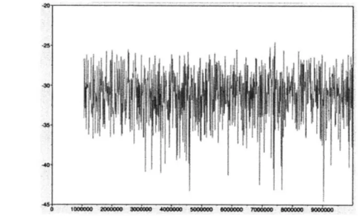
After an MCMC run is completed, one should check that the chain has reached convergence before using the results. One way of checking this is by observing the trace

plot of the likelihoods, such as the one shown below:

430

Figure 1.1: A sample trace plot. The x-axis is the number of iterations, and the y-axis is the posterior likelihood.

The "hairy caterpillar" pattern that can be seen in Figure 1.1 is an indication that convergence has been reached. The period before convergence is reached, known as the

burn-in period, is heavily influenced by the starting point that was chosen by the chain,

(16)

and is therefore generally ignored in the analysis. Furthermore, instead of considering all the parameters that were visited after convergence, one should sample the parameters at a

sampling rate low enough to avoid autocorrelation among successive steps, but high

enough to produce enough samples.

1.3 Comparing Evolutionary Models

Dunn et al. have used the Bayesian phylogenetic method in two different ways in order to analyze the word-order universals. First, based on strings of linguistic characters, which are analogous to DNA sequences in biology, they used the method to find a set of linguistic phylogenetic trees with high posterior likelihoods (see Chapter 2 for the details). Second, they used the set of trees that they obtained to investigate whether the evolution of two word-order traits are correlated. They accomplished that by comparing two different evolutionary models: the independent model, where the two word-orders evolve independently, and the dependent model, where the evolution of one word-order influence the other.

For the independent model, the parameters are which tree among the set to use, and the

transition probabilities of each word-order trait. For example, suppose that each of the

two traits that are compared can exhibit two states, 0 and 1. (If the trait is the ordering of verb and object for instance, then 0 may represent the object-verb order and 1 the verb-object order.) For each trait, there will be two transition probabilities: poi, the probability

(17)

that 0 changes to 1 within a certain time period, and plo, the probability of the opposite change. Thus, there will be four transition probability parameters that specify the independent model.

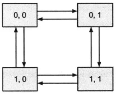
For the dependent model, the parameters are which tree to use and also the transition probabilities. If each trait has two states as before, then there will be eight transition probabilities corresponding to the eight arrows shown in the figure below. Note that the transitions that involve simultaneous changes of the two traits (e.g. (0, 0) to (1, 1)) are not

allowed for simplicity.

Figure 1.2: The state transitions in the dependent model. The two digits in each box represent the states of the first and the second traits.

In order to determine which model is better, one needs to compute the ratio of the

posterior probability of the model,

(1.3)

where MD and M represent the dependent and independent models respectively. A ratio

(18)

larger than one would indicate that the dependent model is preferred, while a ratio smaller than one would indicate the opposite.

In right hand side of Equation 1.3, the term P(MD) / P(I) is set to one if there is no prior bias towards one of the models. Twice of the log of the remaining term is known as the

Bayes Factor (BF), which signifies the strength of support for MD:

BF =2 log [ P(XMD) /P(XMI) ]=2 ( log [ P(XD) ] - log [ P(XMI]). (1.4)

The likelihoods P(XIMD) and P(Xvh) are difficult to compute due to the vast parameter space, but they can be estimated easily using the harmonic mean of the posterior likelihood values from an MCMC run. The problem with the harmonic mean estimator is that it is very unstable because samples with very small likelihoods can have a large effect on the final result; thus, the analysis has to be repeated a few times with very long

MCMC runs (e.g. a billion iterations) (Newton & Raftery 1994). More stable estimators,

such as the thermodynamic integration method (Lartillot & Philippe 2006), have been invented, but they are computationally expensive.

The interpretation of Bayes Factors may vary among authors. Dunn et al. considered BF

> 2 a weak support, BF > 5 a strong support, and BF > 10 an extremely strong support for

the dependent model. Cysouw (2011) consider this interpretation too lenient, mentioning that a strong evidence should require BF > 9.5 based on the calculation suggested in

(19)

independent model, but since the independent model is a special case (i.e. a subset) of the dependent model, this method is inherently not able to provide very strong evidence for the independent model (BF < -5 should be relatively rare).

1.4 Lineage-specific Trends

Dunn et al. used the method described in the previous section to compute the Bayes Factor for each pair among the eight word-order traits for the four language families: Austronesian, Bantu, Indo-European, and Uto-Aztecan. They showed that for for none of the 28 possible word-order pairs is the dependent model consistently strongly preferred (i.e. BF > 5) across the four language families. They also found several strong dependencies between word-order pairs that Dryer claimed to be independent, such as between OBV and DEM (BF = 7.55) in the Indo-European family. They concluded that "most observed functional dependencies between traits are lineage-specific rather than universal tendencies."

Despite the groundbreaking approach, criticisms of this work have been quite numerous. One critique was written by Longobardi and Roberts (2011), which includes three important points. The first one is that the data that was used by Dunn et al., which include merely eight word-order characters, were too small to produce reliable conclusions. The second one is that the validity of the data itself is questionable. An example that was raised was that the verb-object (OBV) orders of some of the modem Germanic languages

(20)

(German, Dutch, Afrikaans, Flemish, and Frisian) were assigned to a "polymorphic state", which indicates that the verb can either precede or follow the verb. This contradicts the general view among contemporary linguists (since 1975) that those Germanic languages are underlyingly always verb-final, and that the verb-second position in Germanic main clauses is a derived structure (Thiersch 1978). The validity or the word-order data of the other less studied languages are even more questionable. The third criticism is that Dunn et al. used the surface (phenotypical) forms of the languages to do the analysis instead of more genotypical parameters derived from formal grammar. Longobardi and Roberts compared their approach to making genetic analysis in biology using phenotypical features.

Others have criticized the way Dunn et al. drew the conclusions from the results. Cysouw (2011) mentioned that while Dunn showed that none of the pairs showed consistent strong support (BF > 5) for the dependent model, the Bayes Factors of four of the pairs, namely ADP-OBV, ADJ-GEN, OBV-SBV, and ADP-GEN, are consistently greater than 2 across the four language families, indicating a universal positive support. Furthermore, Levy and Daum6 (2011) mentions that a low BF for a word-order pair merely indicates the lack of evidence for the dependent model, but one cannot jump from that to the conclusion that the dependency do not exist, or as they eloquently put it: "Dunn et al. have presented the strength of evidence for an effect but interpreted it as the strength of the effect itself." Levy and Daum6 also noted the low BFs are often caused by the lack of variation in one of the traits. For example, there's virtually no variability in the DEM feature in the Uto-Aztecan family (it is always demonstrative-noun except in one

(21)

language), and thus, unsurprisingly, none of the traits have strong dependency with DEM in the Uto-Aztecan family.

All of these criticisms reveal important flaws in the work by Dunn et al., but the focus of

this thesis is to examine the preciseness and the accuracy of the Bayesian analysis that is applied to this particular problem. In the subsequent chapters, we will attempt to reproduce their results and modify their experiments to examine the reliability and the

(22)

(23)

Chapter 2

BayesPhylogenies: Building Phylogenetic Trees

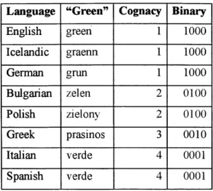
BayesPhylogenies is a software package developed by Mark Pagel and Andrew Meade to construct phylogenetic trees using Bayesian Markov chain Monte Carlo (MCMC) method. In biological uses, the program takes as an input a genomic sequence (a string of nucleobases) of a certain length for each species, and outputs the most likely phylogenetic tree after a number of iterations. In the case of human languages, the analog for genomic sequences would be a string of linguistic characters, features of a language that can take one or more states (i.e. forms) (Nakleh et al. 2005). The characters that were used by Dunn et al. were lexical characters, which represent the existence or non-existence of certain cognates of meanings in the Swadesh list. Below is an example for the meaning "green", taken from the Indo-European data collected by Dyen et al.

(1997)2:

(24)

Table 2.1: The word "green" in several Indo-European languages

In the table above, the words were divided into four color-coded cognate groups. In the

last column, one can notice that the number of binary digits is the same as the number of

cognates, and each digit represents the existence of a cognate in the language.

A complication of this method is that it may be difficult to judge whether a group of

words are cognate or not. Dyen's data, from which Dunn's Indo-European lexical data is derived, label each cognacy as either "cognate" or "doubtfully cognate"; however, it is

unclear how Dunn et al. treated the lexical items that were "doubtfully cognate". Another

problem is that a language may own a cognate due to borrowing. According to Dunn et

al., such cases are usually easy to detect and are removed from the list.

In this chapter, the phylogenetic trees that are necessary for the Bayesian analysis in

Dunn et al.'s paper were reproduced and compared with the published trees. The attempt Language "Green" Cognacy Binary

English green 1 1000 Icelandic graenn 1 1000 German grun 1 1000 Bulgarian zelen 2 0100 Polish zielony 2 0100 Greek prasinos 3 0010 Italian verde 4 0001 Spanish verde 4 0001

(25)

Austronesian trees is too computationally intensive and we did not have the lexical data for the Uto-Aztecan family.

2.1 Indo-European Trees

In order to reconstruct the Indo-European phylogenetic trees that will be used for the comparison of the dependent and independent evolutionary models (Chapter 3), we used the lexical file, containing linguistic characters representing the cognates of Swadesh words, that was kindly supplied by Dunn. In the supplementary information published along with the 2011 paper, Dunn et al. commented as follows about the source of the data:

The Indo-European lexical data based on the published dataset of Dyen et al. (1992). We used a substantially expanded version of the data described in Gray and Atkinson (2003) with 82 distinct languages (including 8 new to this study) and 4049 cognate sets.

Although Dunn et al. reported the data covered "82 distinct languages", in fact only 78 appeared in the corresponding paper. Moreover, although they mentioned that there were 4049 cognate sets in this dataset, there were only 2301 characters per language in the file Dunn supplied for this current study. Thus, the Swadesh file used for the re-analysis may be incomplete. Furthermore, although the file contained data for 101 languages, 23 of them do not appear in their paper, (leaving 78 languages). The 23 missing languages are:

(26)

AlbanianC AlbanianK Albanian Top Albanian_T

AnnenianList GreekK GreekD GreekMd

Greek_Ml Khaskura GypsyGk Czech_E

Lithuanian_0 Swedish_Vi Swedish Up Brazilian

SardinianL SardinianN Vlach BretonSe

BretonList WelshC Irish_A

Those languages mostly correspond to the languages where the word-order data (used for the subsequent correlated evolution analysis) are not available in the World Atlas of

Language Structures.

Since there are 101 languages in the data file, but only 78 languages are needed, there are two ways to build trees with 78 leaves. The first way is to reduce the data file to 78 languages, and then build the trees (pre-prunning); the second way is to build trees with 101 languages, and then prune the 23 undesired leaves (post-pruning). According to

Greenhill, one of the co-authors of Dunn et al.'s 2011 paper, the second way is preferred

because the trees produced match the expected subgroupings better. However, there is no theoretical reason why one way should be better than the other, and therefore we proceed to examine the trees produced from both methods.

Following the method given by Dunn et al.'s Supplementary Methods, phylogenetic trees were generated by running BayesPhylogenies for 5 million iterations on the lexical data (both pre-pruned and unpre-pruned), with 2 million bum-in period and sampling rate of 5000, leaving 601 trees in the sample. Following the Anatolian theory of IE origin, as

(27)

The phylogenetic analysis shows that the language family trees are still divergent after 5

million iterations. Adding more iterations (up to 100 million) does not mitigate the problem because the lexical data provided by Dunn are too small to resolve some of the ambiguities in the trees, such as position of the Albanian branch, or the position of the Romance branch with respect to the Germanic and the Slavic branches.

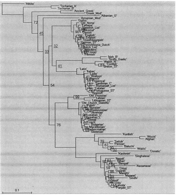
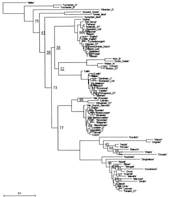
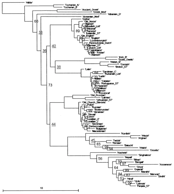
Figure 2.1 below shows the consensus tree obtained from the first way described above (reducing the lexical file to 78 languages) with 5 million iterations. Figures 2.2 and 2.3 are the consensus trees obtained from the second way (pruning the trees after they are built with 101 languages), with 5 million and 100 million iterations respectively. Figure 4 is the consensus tree of the trees that Dunn gave us along with the Swadesh files; it is not identical to the published tree in Dunn et al.'s paper.

(28)

(29)

'Hite'

'AbanianG'

- 'O~ssetic'

ASisaese

(30)

'Hitie -AIanian -Xurcish' -singhalese N epW ar elw 0.1 'PajbST

(31)

'Ajbmanng 73 ltdslh M4arwer 4 9 "Wap.-10 PanjabiST

(32)

Compared to the consensus tree that was published in Dunn et al.'s paper, while the positions of most branches in the four consensus trees are the same, there are several differences. The positions of Armenian, Albanian, the Celtic branch, and several other languages are different. The differences reflect the inherent ambiguity in the positions of those branches, as can be seen from their low bootstrap values. Another difference is that

Old Prussian is not shown in the published tree.

There are also differences among the four trees. Figure 2.1, 2.2, and 2.3 are relatively similar. In particular, Figure 3 is almost identical to Figure 2, indicating that 100 million iterations do not produce better results than just 5 million. Figure 2.4 is significantly different from the other three figures because the branch lengths are significantly longer (notice to the scales at the bottom left of the figures). It remains to be determined what causes the difference, and what effect the difference has to the results of the correlated evolution analysis.

2.2 Bantu Trees

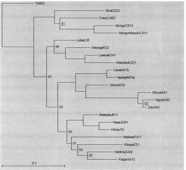
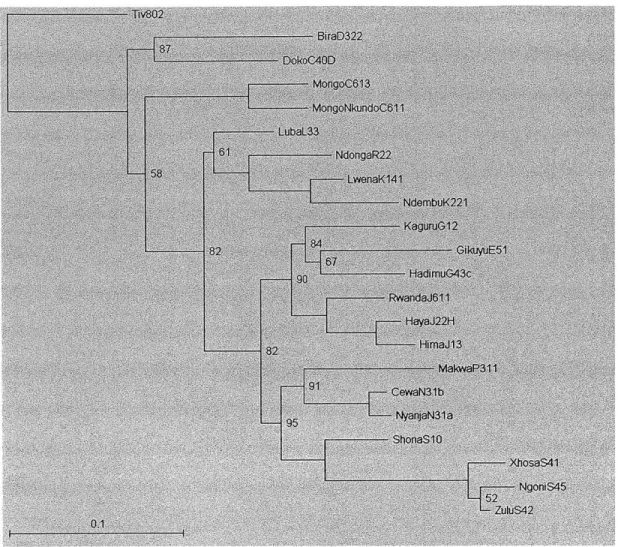
The Bantu trees were built using a similar method as the Indo-European trees, using the lexical file that was kindly provided by Greenhill. The lexical file contains 95 languages, but only 48 are used in the paper. As before, the trees are built in two ways: pre-pruning and post-pruning. Following Dunn et al., the trees were generated by running BayesPhylogenies for 5 million iterations on the lexical data, with 2 million bum-in

(33)

period and sample period of 5000, leaving 601 trees in the sample. Following the paper, the trees are rooted at Tiv. In the figures below, the trees are further pruned to 22 languages in order to allow easy comparison with Figure 1 in Dunn et al.'s paper.

-BiroD322 Dok oCA0D MongoC613 MongoNkundoCM11 LubaL33-81 NdongaR22 LwenaK141 NdembuK221 -CowaN31 b 97 Nyaa1 ShonaS10 XhosaS41 NgoniS45 --- 82 ZUS42 RwwandJ611 HayaJ22H --- 93fim&113 MoloaP311 58 Kaguru12

(34)

Figure 2.6: Consensus tree obtained with post-pruning, 5 million iterations

Comparing the two trees to the published tree (Figure 1 of the paper) qualitatively, it

(35)

Chapter 3

BayesTraits: Detecting Possibly Correlated

Evolutionary Traits

BayesTraits is a computer package, also developed by Mark Pagel and Andrew Meade, to analyze correlated evolution between two biological traits, for example to answer the question of whether mating system and advertisement of estrus by females have coevolved in the great apes. In the case of human languages, a possible corresponding analog is a measure of whether the evolutions of two word orders in different natural languages are likely to be correlated.

In the DISCRETE mode, BayesTraits takes a collection of phylogenetic trees and two sets of trait data (in Dunn et al.'s case, word-order data) as input, and outputs the likelihood of the model under two assumptions: (1) independent/uncorrelated traits (M) or (2) dependent/correlated (MD) traits. These likelihoods are approximated using the Markov chain Monte Carlo (MCMC) method. As mentioned in Section 1.3, the models are tested by computing the Bayes Factor (BF) using the harmonic likelihood estimator. Following Dunn et al., a BF greater than 5 indicates the evolutions are likely to be correlated.

(36)

The purpose of this chapter is to test the robustness of Dunn et al.'s approach by applying various modifications to their original experiments. Our reanalysis is limited to the Indo-European language family because we could not reproduce the phylogenetic trees for the Austronesian and Uto-Aztecan families, and the dataset for the Bantu family is too small and homogeneous. For all of the Indo-European analysis in this chapter, the 5 million iteration post-pruned trees (Figure 2.2) were used.

3.1 Initial Test

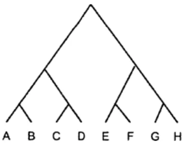
To test how BayesTraits functions, an artificial tree with eight leaves as shown in Figure

3.1 and two sets of artificial data in Table 3.1 were created.

A B C D E F G H

(37)

Data A species ABC D E F GH trait1 0 0 1 1 0 1 0 1 trait2 0 0 1 1 0 1 0 1 Data B species A B C D E F G H trait1 0 0 1 1 0 1 0 1 trait2 0 1 0 1 00 1

Table 3.1: Trait data for the tree in Figure 3.1

It can be observed that in Data A, traiti and trait2 appear to be dependent because every change from state 0 to state 1 in trait1 is accompanied by the same change in trait2. In Dataset B, however, trait1 and trait2 seem to be independent of one another. Unsurprisingly, BayesTraits produces BF = 11 for Data A and BF = 0 for Data B.

3.2 Stability of Harmonic Mean Estimator

As mentioned in Section 1.3, the least computationally expensive way to estimate the Bayes Factor is by computing the harmonic means of the posterior likelihoods from the stationary phase of an MCMC run. The harmonic mean is defined as

(3.1)

where x1, x2, ... , xn are the likelihoods during various sample points throughout the run,

and n is the number of points. The BayesTraits manual and other phylogenetic literature recommend using the harmonic mean estimator, but wams that it may be unstable, and therefore each MCMC chain has to be run for many iterations (e.g. 100 million) and

(38)

repeated a few times (e.g. five times).

The purpose of this section is to measure the stability of the harmonic mean estimator. Seven dependent and seven independent runs with 50 million iterations each were run on the ADP versus OBV traits, with a sampling rate of 10000. The results of the runs have sufficiently converged, as can be seen in the superimposed likelihood density plots of the fourteen runs in Figure 3.1 below. The left peak corresponds to the independent runs, and the right the dependent runs. The seven plots of each model lay almost on top of each other. The trace plot of each run also exhibits the "hairy caterpillar" pattern as shown in Figure 1.1, indicating convergence.

0.3-OM5

02;

015

Figure 3.2: Superimposed likelihood density plots of seven independent runs and seven

(39)

However, the harmonic means of the 50 million iteration runs have not converged. The problem is that since the harmonic mean is based on the reciprocals (1/x) of the inputs, it gives disproportionately large weights to inputs with very small likelihoods. The box and whisker plots in Figure 3.3 below show the distribution of the harmonic means of the seven independent and dependent runs. The BFs based of this estimator can vary from 4.8 to 22.3, which is a huge range. (Dunn et al. reported BF = 13.34 for this pair.) Figure 3.4 is a similar plot, but based on independent dependent runs that were executed for one billion iterations each. It appears that doing more iterations does not mitigate the problem.

ADP vs OBV 50M, BF range: 4.847~ 22.2827

-54 -56 0o 0 -62 -64 Independent Dependent

Figure 3.3: Box and whiskers plots for the dependent and independent likelihoods of the

(40)

V 0 0 0 -J -53 -54 -55 -56 -57 -58 -59 -60 -61 -62 -63

ADP vs OBV, BF range: -0.96444 ~ 17.076E

Independent Dependent

Figure 3.4: Same as Figure 3.3, but each value is taken from the harmonic mean of a 1 billion iteration run. Dunn et al. reported BF = 13.34.

We have repeated the analysis for the other eight word-order pairs that were reported by Dunn et al. as being strongly correlated in the Indo-European family. The box and

whiskers plots for those pairs can be found in Appendix A. Most of them also show the

large variations we found for the ADP-OBV pair (Figure 3.4). Furthermore, in five of the

pairs, we were not able to reproduce the high BFs Dunn et al. reported.

In order to show the inherent stability problem with the harmonic mean, it is useful to

compare it with the geometric mean, which is defined as

G = (x1 -x2 * ... * xn) "" . (3.2)

The geometric mean can be computed easily by taking the arithmetic mean of the log

(41)

of the independent and dependent 50 million iteration runs. It can be immediately seen that the geometric means have converged very well, a sharp contrast with the distributions we saw in Figure 3.3.

ADP vs OBV 50M (G), BF range: 15.774 ~ 16.17E

-49 _ -502 -54 -.55 -56 -57 Independent Dependent

Figure 3.5: Same as Figure 3.4, but each value is computed based on the geometric mean of a 1 billion iteration run.

If we were to compute BFs based on the "geometric mean estimator", it would vary from 15.8 to 16.2, which is a very small range. This range is incidentally close to the BF

computed from the medians of the harmonic means, 15.1. However, there is no mathematical proof that the "geometric mean estimator" would converge to the quantity defined in Equation 1.4. Nonetheless, the geometric means show us that even though the runs have statistically converged very well, the mathematical properties of the harmonic mean prevent it from converging. These also show that the Bayes Factors that were reported by Dunn et al. are based on an estimator that have not converged, and thus one may not be able to reproduce their results even if identical parameters are used.

(42)

3.3 Bayes Factor Sensitivity to Errors

Two experiments were designed to check the sensitivity of the Bayes Factor computations to small changes in the data. In order to keep them tractable, the experiments are limited to the ADP-GEN traits of the 23 Indo-European languages that are in the Indo-Iranian branch. In the absence of any modification, the ADP-GEN Bayes Factor of those languages, computed from 10 million iteration MCMC runs, was 5.35, indicating a fairly strong correlation.

In the first experiment, the 23 Indo-Iranian languages were put in a random order, and then 23 order matrices were generated. (The matrix is the file containing the word-order data. Each matrix has two columns representing the ADP and GEN traits, and 23 rows representing the 23 languages.) In the n-th matrix, the ADP traits of first n languages are flipped, meaning that if the trait is 0, it will be changed to 1, and vice versa. It means that the n-th and the (n+1)-th matrix are always different by only one digit. The BF of each matrix is computed with 10 million iterations. The whole experiment was repeated three times, with three different random orderings of languages, and the results are plotted in Figure 3.6.

(43)

Z5 0 -- - ---1 05 10 15 20 Numrber of Flips -4 -E -0o -20 5 10 15 20 Nurnber of Flips 10 --'4 ai2 -10 -- --- - -- - -- --- --- - --- ---LL -4 0 5 to 1s 20 Nurnber of Flips

Figure 3.6: Each plot represents one repetition of the first experiment. The red dashed lines are

(44)

In the plots above, one can see that the adjacent BFs are mostly different by only a small amount; this is expected because they are only different by one digit in the matrices. However, occasionally the BF jumps quite dramatically. For example, between 16 and 17 flips in the second figure, the BF increases by about 10. It shows that while one-digit

errors usually do not affect the computation by much, sometimes it can have a dramatic impact.

Note that the BFs always dip to negative values when the ADP traits of about half of the languages are flipped. This is to be expected because in that situation, the relationship between the two traits is essentially random, and a random relationship is more likely to be independent than dependent. Note also that after flipping 23 times, the BF returns to near the original value. This is because flipping the ADP traits of all languages is equivalent to switching the notations of the two possible ADP states (i.e. switching 0 and

1), and thus the relationship between the two traits is unaltered.

In the second experiment, 23 matrices are also generated, but in the n-th matrix, only the

ADP trait of the n-th language is flipped. Thus, each of the 23 matrices is only different by one digit from the original data. The Bayes Factor of each matrix is computed with 10

million iterations, and the distribution of the results is shown in the box and whiskers plot in Figure 3.7. The magenta dashed line indicates the original BF.

(45)

Q -10 8 0 L 4 2

Figure 3.7: The distribution of the 23 Bayes Factors from the second experiment. The magenta

dashed line indicates the original Bayes Factor.

Again, this experiment shows that most one-digit errors do not alter the Bayes Factor by

much. The first and the third quartiles of the distribution are within ±1 of the original BF.

As a comparison, the BFs of the original data also vary by around ±1 across different

runs (measured by standard deviation). However, some errors can alter the BFs

substantially, dropping it down to 0 or raising it up to 12; this is another evidence that an

error as small as one digit can have a dramatic impact on the final result. Therefore, it is

important that each point in Dunn et al.'s trait data is verified, and it is alarming that an

(46)

3.4 BayesTraits and Polymorphism

In the DISCRETE mode of BayesTraits, the trait data must be binary: either 0 or 1 for each trait. (Hyphens can be used for missing data.) In the cases where the trait is uncertain, or where the trait appears to be polymorphic (multivalued beyond binary) in a certain species, it still has to be labeled as either 0 or 1 (or as missing). In Dunn et al.'s paper, it was reported that word-order traits were polymorphic in many languages. For example, contrary to the general consensus among linguists (e.g. Thiersch 1978), they claimed that an object in German can either precede or follow the verb. They notated such polymophic data as 01. However, several months after they carried out their analysis, we discovered through an examination of the source code of BayesTraits, kindly provided by one of its authors, Meade, that an input 01 will be truncated into 0 (see Appendix B for details). Consequently Dunn et al.'s corresponding published calculations are flawed. Following this discovery, Meade noted that polymorphic data should be coded as a hyphen (-), that is, as if it were missing data.

It is therefore necessary to examine their dataset to determine what proportion might have been affected by this coding error as well as whether the error makes a different in the computed output results.

Table 3.2 below shows the number of traits that were reported as polymorphic (01) in each language family. The column "Any" is the number of languages that have at least

(47)

one polymorphic trait among the eight word-order traits. The column "# Langs" is the total number of languages in the family.

Family Indo-European Austronesian Bantu Uto-Aztecan ADJ ADP 3 4 12 2 2 0 5 1 DEM 2 1 0 1 GEN NUM 14 3 6 9 0 1 2 0 OBV 11 1 0 5 REL 5 4 0 2 SBV 10 6 4 3 Any 4 40: 33 5 25 Langs 77 127 48 25

Table 3.2: The number of polymorphic traits in each language family

Table 3.3 displays the same numbers as percentages:

Family Indo-European Austronesian Bantu Uto-Aztecan ADJ 3.9 9.4 4.2 20.0 ADP 5.2 1.6: 0.0 4.0 DEM 2.6 0.8 0.0 4.0 GEN 18.2 4.7 0.0 8.0 NUM 3.9' 8.11 2.1 0.0 OBV 14.3 0.8 0.01 20.0 REL 6.5 3.1 0.0 8.0 SBV 13.0 4.7 8.3 12.0 Any 51.9 26.0 10.4 44.0 # Langs 77 127 48 25

Table 3.3: The percentage of polymorphic traits in each language family

These tables show that polymorphisms might most affect Dunn's BF calculations for the

Indo-European and Uto-Aztecan language families.

The 01 notation, however, do not always cause a mistake. For example, according to

(48)

English, German, Dutch, Afrikaans, Flemish and Frisian are not 01 (polymorphic) as reported by Dunn et al., but 0, representing verb-final (Thiersch 1978, Longobardi & Roberts 2011). Since 01 is truncated to 0 by BayesTraits, they inadvertently arrived at the correct data.

3.5 Labeling Polymorphic States as Missing

Following the suggestion by Meade, Dunn et al.'s computations were repeated, but using hyphens (indicating missing data) instead of 01 to label the polymorphic states. The computations using 01 were also repeated for comparison. Each MCMC run was executed for one billion iterations and repeated between one to eleven times, and the likelihoods were computed using the harmonic mean estimator.

While Dunn et al. repeated each run six times, they only published the BF obtained from the medians of the harmonic means. However, in order to display the actual spread, we show the distribution of all the possible BFs from our runs: if the dependent run is repeated m times and the independent run n times, then there are m-n possible BFs corresponding to every possible pairings. The distributions of the m-n BFs for five word-order pairs are shown in Figure 3.8. The left and right plots use 01 and hyphen for the polymorphic states respectively. The magenta dashed line in each plot is the BF reported

by Dunn et al. The distributions of independent and dependent likelihoods corresponding

(49)

ADP vs GEN 20 18 is o 14 I-L- 12 0) 8 6 4 01 hyphen ADP vs OBV 20 -0 15m LL w 10 0 01 hyphen DEM vs GEN 8 6 -4 0 --6 01 hyphen

(50)

LL ci) 0 0 i-(0 8 6 4 2 0 -2 -4 -6 -8 -10 6 4 2 0 -2 -4 DEM vs OBV 01 hyphen GEN vs OBV ---01 hyphen

Figure 3.8: The distribution of the Bayes Factors obtained from 1 billion iteration runs. The left

and right plots use 01 and hyphen for the polymorphic states respectively. The magenta dashed lines indicate the BFs reported by Dunn et al. (2011). Compare these plots with the independent

(51)

For all word-order pairs, the BF ranges are substantial for both the 01 and the hyphen results. One fact that is not displayed in the figure is that when hyphen is used, the dependent and independent likelihoods are always higher. This is because the "missing" data are ignored by BayesTraits, and therefore the parameter space of the model becomes smaller. Ignoring that, it appears only in one case, ADP-OBV, is Dunn et al.'s BF located within the first and third percentile of our 01 BF range. In one case, ADP-GEN, our hyphen BFs match Dunn et al.'s BF better than our 01 BFs. In the three other cases, Dunn et al.'s results are not reproduced.

3.6 Branch Analysis

Finally, a small-scale experiment was run to examine Dunn et al.'s claim that the

word-order universals are lineage-specific. The Indo-European languages were divided into the Balto-Slavic branch (16 languages), Germanic branch (16 languages), Indo-Iranian branch (23 languages), and Romance branch (11 languages) according to their phylogenetic classifications. For each of the four branches, the Bayes Factors for the

ADP-GEN, ADP-OBV, and GEN-OBV pairs were computed with 10 million iteration MCMC runs. The results are shown in Table 3.4.

(52)

Balto-Slavic Germanic Indo-Iranian Romance all IE (Dunn et al)

ADP-GEN -1.83 -1.98 5.35 1.90 13.65

ADP-OBV -3.12 -2.13 -3.07 -0.54 13.34

GEN-OBV 0.41 0.08 -2.68 -0.23 5.27

Table 3.4: The BFs of the four major Indo-European branches. The last column contains the BFs published by Dunn et al. for the entire Indo-European tree.

Although Dunn et al. reported high BFs (greater than 5) for those three word-order pairs, and our results in Figure 3.8 also verify it, none of the branch BFs in the Table 3.4 display positive correlation (BF > 2) other than the ADP-GEN pair of the Indo-Iranian branch. Superficially, it seems to support Dunn et al.'s claim that the word-order universals are lineage specific: if we consider the four branches as separate lineages, then our results demonstrate that the "word-order universals" are not universal; the ADP-GEN correlation is specific to the Indo-Iranian lineage. However, the flaw in this reasoning is apparent. The low BFs are a reflection of the sample sizes that are too small and the lack of variability inside the branches; for example, in the Romance branch, the ADP trait is always 1, representing prepositions. Although the BFs are low, we cannot say that the traits do not correlate evolutionarily since there is the possibility that the data is not diverse enough to display the trend. This is exactly the logical fallacy in Dunn et al.'s conclusion: the absence of high BFs in some of the language families cannot be taken as an evidence for the lineage-specificity of the word-order universals.

(53)

Chapter 4

Conclusions

4.1 Summary of Findings

In this thesis, I have analyzed the Bayesian phylogenetic analysis that was ingeniously employed by Dunn et al. (2011) to test the correlation among the evolutions of word-order traits. The effectiveness of this approach boils down to two points: whether the results are reproducible, and whether the results are accurate.

This thesis has demonstrated that many of the results by Dunn et al. cannot be reliably reproduced. In Chapter 2, it was shown that the phylogenetic trees that were built based on their lexical data contain many nodes with low bootstrap values, and therefore the consensus trees that are produced by different runs often have distinct structures. In Chapter 3, it was shown that results of the correlated evolution analysis (the Bayes Factors) were very uncertain as well. The experiment in Section 3.2 shows the harmonic mean estimator, which was employed by Dunn et al., was so unstable that the Bayes Factors of different runs may vary widely. The plots in Appendix A show that we could not reproduce many of the Bayes Factors reported by Dunn et al. This is further coupled

(54)

with the results in Section 3.3, which demonstrates that a single digit error in the traits data can have a significant impact on the Bayes Factor. All of these complications show that the whole computation is so unstable and sensitive to tiny changes that most of the results are irreproducible.

Furthermore, this thesis has revealed several errors in the computational method itself. Sections 3.4 and 3.5 describe our finding that the notation '01' that Dunn et al. used to encode polymorphism was an invalid input to BayesTraits, and the correct notation should by a hyphen, indicating a missing data point. Figure 3.8 and Appendix C show that this error has a significant impact to the likelihood and Bayes Factor calculations. Finally, Section 3.6 demonstrates that Dunn et al.'s conclusion that the word-order universals are "lineage-specific" does not logically follow from their results.

While this thesis has demonstrated that the results reported by Dunn et al. are erroneous and unreliable, these findings should not be interpreted as an argument against using Bayesian approaches in the domain of philology. This novel approach may have a big role in understanding the interplay between lineage and linguistic typology, but the implementation needs to be refined so that the results drawn from it can be trusted.

(55)

4.2 Future Work

Future work should focus on developing the Bayesian approach so that it is more usable in the domain of computational linguistics. There are several points that need to be addressed in order to achieve this goal. The first one is determining the effect of using phylogenetic trees with low bootstrap values to the results of the correlation analysis. This is important because very often the lexical data one has (in both linguistics and biology) is not adequate to resolve some of the ambiguities in the phylogeny. The second one is finding a way to produce stable results with the harmonic mean estimator (e.g. by doing a huge number of runs), or examining the feasibility of using other estimators that are more reliable, but more computationally expensive. The final one is investigating the other uses of the Bayesian approach in the philology analysis, which include the computation of the transition probabilities between different states (i.e. the thickness of the arrows in Figure 1.2) and reconstruction of the ancestral states.

(56)

(57)

Appendix A: Likelihood and Bayes Factor plots of Indo-European word-orders

The figures on the left side are the box and whiskers plots of the independent and dependent likelihoods of nine Indo-European word-orders that were reported as being strongly correlated (BF > 5) by Dunn et al. The likelihoods are computed using on the

harmonic mean estimator. Each MCMC run was conducted for one billion iterations and repeated between one to eleven times.

The figures on the right side are the box and whisker plots of the possible Bayes Factors (BFs) corresponding to the likelihood values in the left figures. If the dependent run is repeated m times and the independent run n times, then there are m-n possible BFs corresponding to every possible pairings. The plots show the distributions of the m n BFs. The magenta dashed line in each plot is the BF reported by Dunn et al.

ADJ vs DEM ~-independent Dependent ADJ vs GEN Independent Dependent ADJ vs DEM 8 6 0 C2 U-0 -2 -4 27 26 ADJvsGEN 25 1 0 i5 CO LL C/) C) 0 24 23 22 . 21--20 19 -35.5 -36 -36.5 I. -37 [ -37.5 -38 -38.5 -a 0 0 (D 0 _j 'a00 C_ -62 -64 -66 -68 -70 -72 -74

(58)

---ADJ vs SBV ADJ vs SBV Independent Dependent ADP vs GEN Independent Dependent ADP vs OBV Independent Dependent 5 0 U-'D-10 -15 -32 -34 -36 -38 -40 -42 -44 -46 -48 -50 0 LL 0] 16 14 12 ADP vs GEN T1~ 101. 8 6 4 ADP vs OBV 20 [ 0 U-(0, 0 i5 10 1. 5 0 V -J 0 -J -20

2

-64 -65 -66 0 o -67 S-68 Cb-69 -i -70 -71 -72 -56 -58 0 ~ -60 b-62 -64 -66

(59)

V 0 0 -J 0 -J Independent Dependent 75 LL 03) 8 6 4 2 0 -2 -4 -56 DEM vs GEN -56.5 -57 -57.5 -58 -49.5 -50 -50.5 -51 DEM vs GEN Independent Dependent DEM vs OBV Independent Dependent GEN vs OBV

--

5

0 ,Z5 (0 U-md 7 6 5 4 3 2 1 0 8 6 2 0 15 -2 -4 V 0 0 -J 0 -J -T-DEM vs OBV GEN vs OBV -51.5 -83.5 -84 -84.5 -85 o,-85.5 -86 -86.5

(60)

~-GEN vs SBV Independent Dependent t EL £1) GEN vs SBV -58.2 -58.3 -58.4 -58.5 -58.7 -58.8

(61)

Appendix B: Excerpts from BayesTraits source code

The code starts with the function Setupoptions in initialise.c. In order to validate the input data, the function calls CheckDataWithModel in data.c, which calls CheckDescData if the model is DISCRETE. This function checks if the input data is valid by calling ValidDescDataStr:

int ValidDescDataStr(char* Str) { while(*Str != '\0') { if(!((*Str == '0') || (*Str == 'l') || (*Str == return FALSE; Str++; } return TRUE; }

This function only checks if the data only contains 0', '1 or '-'. This function does

not care about the length of the data. For example, one can input '0101-01-' and this function will return FALSE.

IfValidDescDataStr returns FALSE, then CheckDescData will message: "Taxa %s has invalid discrete data for site and - are valid discrete data character.\n". This error imply that ' 01' is not a valid input.

print the error %d.\nOnly 0,1 message seems to

Otherwise, if ValidDescDataStr returns TRUE, then SetUpOptions will call the next function, CreatOptions in options.c. If the model is DISCRETE, it will call SquashDep in data. c. One part of the function is:

if((Taxa->DesDataChar[0][0] == '0')

&& (Seen == FALSE))

{ Taxa->DesDataChar[0][0] = '0'; Taxa->DesDataChar[0][1] = '\0'; Seen = TRUE; } if((Taxa->DesDataChar[0][0] == '0')

&& (Seen == FALSE))

{ Taxa->DesDataChar[0][0] ₌ 'l'; Taxa->DesDataChar[0][1] =-\' Seen = TRUE; } if((Taxa->DesDataChar[0][0] == '1')

&& (Seen == FALSE))

{ Taxa->DesDataChar[0][0] ₌ '2'; Taxa->DesDataChar[0][1] =-\' && (Taxa->DesDataChar[1][0] == '0') && (Taxa->DesDataChar[1][0]== '1') && (Taxa->DesDataChar[1][0]== '0')

(62)

Seen = TRUE; }

if((Taxa->DesDataChar[O][0] == '1') && (Taxa->DesDataChar[1j[0]== '1') && (Seen == FALSE))

{

Taxa->DesDataChar[O][0] = '3';

Taxa->DesDataChar[0][1] ='\;

Seen = TRUE;

I

In the code above, if thefirst character of the first trait is ' ' and thefirst character of the second trait is '0', then they will be represented by '0' (i.e. 0 0 becomes 0).

If thefirst character of the first trait is ' 0 ' and thefirst character of the second trait is

' 1 ', then they will be represented by '1 ' (i.e. 0 1 becomes 1). Similarly, 1 0 becomes 2,

and 1 1 becomes 3. This function ignores everything that comes after the first character,

(63)

Appendix C: Comparison of likelihoods plots using '01' and '-' to encode polymorphic states

The figures below are the box and whiskers plots of the independent and dependent likelihoods of five out of nine Indo-European word-orders that were reported as being strongly correlated (BF > 5) by Dunn et al. The likelihoods are computed using on the

harmonic mean estimator. Each MCMC run was conducted for one billion iterations and repeated between one to eleven times. In the left figures, following Dunn et al., the polymorphic states were encoded using '01', which will be truncated into '0' by BayesTraits. In the right figures, the polymorphic states were encoded using '-' (hyphen), as suggested by Meade. (See Sections 3.4 and 3.5 for the details.) Each pair of figures (left and right) is drawn using the same y-axis (log likelihood) scale for easy comparison. Compare these plots with Figure 3.8, which shows

corresponding to the likelihood distributions below.

ADP vs GEN (01) Independent Dependent ADP vs OBV (01; Independent Dependent -50 -55 -60 -70 0 -70 -40 -45 0 0 :9 -50 0 -60 -65

the Bayes Factor distributions

ADP vs GEN (hyphen)

Independent Dependent

ADP vs OBV (hyphen

Independent Dependent -50 -55 0 0 8) 0 -50 0 _j, -65 -70 -40 -45 -55 -60 -65

(64)

-49 -50 -51 V -52 8-_-53 .~-54 -55 0 -56 -57 -58 -59 -30 -35 0 -45 -50 -60 -65 Independent Dependent DEM vs GEN (01) Idependent Dependent DEM vs OBV (01: Independent Dependent GEN vs OBV (01; -I --I -I