A unified model for rubble ice load and behaviour

Publisher’s version / Version de l'éditeur:

Vous avez des questions? Nous pouvons vous aider. Pour communiquer directement avec un auteur, consultez la première page de la revue dans laquelle son article a été publié afin de trouver ses coordonnées. Si vous n’arrivez pas à les repérer, communiquez avec nous à PublicationsArchive-ArchivesPublications@nrc-cnrc.gc.ca.

Questions? Contact the NRC Publications Archive team at

PublicationsArchive-ArchivesPublications@nrc-cnrc.gc.ca. If you wish to email the authors directly, please see the first page of the publication for their contact information.

https://publications-cnrc.canada.ca/fra/droits

L’accès à ce site Web et l’utilisation de son contenu sont assujettis aux conditions présentées dans le site LISEZ CES CONDITIONS ATTENTIVEMENT AVANT D’UTILISER CE SITE WEB.

National Research Council of Canada PERD Ice/Structure Interaction Program; no. PERD/CHC 5-119, 2005-12

READ THESE TERMS AND CONDITIONS CAREFULLY BEFORE USING THIS WEBSITE.

https://nrc-publications.canada.ca/eng/copyright

NRC Publications Archive Record / Notice des Archives des publications du CNRC :

https://nrc-publications.canada.ca/eng/view/object/?id=6bed09e8-2a70-418a-b8ec-a233425d523d https://publications-cnrc.canada.ca/fra/voir/objet/?id=6bed09e8-2a70-418a-b8ec-a233425d523d

For the publisher’s version, please access the DOI link below./ Pour consulter la version de l’éditeur, utilisez le lien DOI ci-dessous.

https://doi.org/10.4224/12327958

Access and use of this website and the material on it are subject to the Terms and Conditions set forth at

A unified model for rubble ice load and behaviour Brown, T.; El Seify, M.

Final Report

On

A Unified Model for Rubble Ice Load and Behaviour

To

National Research Council of Canada PERD Ice/Structure Interaction Program

PERD/CHC 5-119.

By

T.G. Brown and M. El Seify Department of Civil Engineering

The University of Calgary

Table of Contents

1 Introduction...iii 2 Characterization of Ice Rubble... 2-1 2.1 Problem Definition ... 2-1 2.2 Geometry and Physical Properties of First Year Ridges ... 2-1 2.3 Mechanical Properties of First-Year Ridges ... 2-4 2.4 Shear Strength of First Year Ridge Keel ... 2-5 2.4.1 Laboratory Tests ... 2-6 2.4.2 In-situ Tests ... 2-7 2.5 First Year Ice Ridge Failure Modes and Load Calculation ... 2-13 3 Comparison Between Measured Loads and existing Theories ... 3-1 3.1 Existing Load Models for Rubble Failure... 3-1 3.1.1 Overview of Existing Analytical Keel Load Models – Local Failure... 3-1 3.1.2 Overview of Existing Analytical Keel Load Models – Global Failure ... 3-4 3.2 Modified Consolidated Layer Flexure Load Model Used in the Comparison . 3-13 3.3 Model Comparisons... 3-15 3.3.1 Croasdale (1998) ... 3-15 3.3.2 Summary of the Events Used in the Comparison... 3-16 3.3.3 Comparison Procedure... 3-17 3.3.4 Comparison Results... 3-18 4 Development and Testing of New Model ... 4-1 4.1 Typical Ice Rubble Failure and Deformation Mechanisms... 4-1 4.2 Limitations of the Mohr-Coulomb Stress Criterion ... 4-2 4.3 Shear-Cap Criterion ... 4-2 4.3.1 Cap Hardening... 4-4 4.3.2 Cohesive Softening... 4-4 4.4 Calibration of Material Parameters... 4-4 4.4.1 Parameters Calibrated by Heinonen (2004) ... 4-5 4.4.2 Other Parameters Calibrated to Fit the Confederation Bridge Recorded Data ……….4-5 4.5 Analysis Procedure... 4-12 4.6 Results of the Analysis ... 4-13 5 Conclusions and Recommendations ... 5-1 5.1 Conclusions... 5-1 5.2 Recommendations ... 5-2 6 References ... 6-1

List of Tables

Table 2-1 Summary of Shear Strength Parameters Resulting from Small Scale Tests (Lemée et.al 2003) ………..2-4 Table 2-2 Summary of the Measured Ice Rubble Shear Properties [Chao (1993)]... 2-6 Table 3-1 Comparison of Methods for Keel Loads [Croasdale (1998)]... 3-15 Table 3-2 Summary of the events used in the comparison ... 3-16 Table 3-3 Difference between the calculated and the recorded loads... 3-18

List of Figures

Figure 2.1 Cross-section of grounded first year ridge (Cammeart and Muggeridge, 1988)... 2-2 Figure 2.2 Typical Actual Keel Profile... 2-2 Figure 2.3 a) Sail height vs keel depth b) Keel depth vs time ... 2-3 Figure 2.4 Regression for shear stress for laboratory experiments (Bruneau, 1996)... 2-5 Figure 2.5 Direct shear test arrangement (Croasdale et al. 2001). ... 2-8 Figure 2.6 Typical load vs displacement in the direct shear test (Croasdale et al.2001) .... 2-9 Figure 2.7 Configuration of the punch shear test (Croasdale et al. 2001) ... 2-10 Figure 2.8 Typical load vs displacements, punch shear tests (Croasdale et al. 2001) ... 2-10 Figure 2.9 Ridge keel punch test (Heinonen and Määttänen 2000)... 2-12 Figure 2.10 Failure modes between ice ridges (lines) and cylindrical structures... 2-12 Figure 3.1 Plug failure planes in a ridge keel ... 3-4 Figure 3.2 Cross section and parameters of a first year ridge (Karnä and Nykänen 2004)

………..3-5 Figure 3.3 Failure mechanism with an inclined slip plane and two vertical slip planes

(Karnä et al. 2001). ... 3-6 Figure 3.4 General passive failure model (Croasdale 1999)... 3-7 Figure 3.5 Cross-section sliding scheme. Figure 3.6 Plan of sliding scheme ... 3-8 Figure 3.7 D ≤ 10m, Figure 3.8 D ≤ 100m ... 3-11 Figure 3.9 Cross over model showing progression of failure loads (Lemée and Brown

2002). ………3-13 Figure 3.10 Recorded Loads Vs Calculated Loads (Dolgopolov, 1975) ... 3-20

Figure 3.11 Recorded Loads Vs Calculated Loads (Prodanovic, 1979) ... 3-21 Figure 3.12 Recorded Loads Vs Calculated Loads (Mellor, 1980) ... 3-22 Figure 3.13 Recorded Loads Vs Calculated Loads (Hoikkanen, 1984) ... 3-23 Figure 3.14 Recorded Loads Vs Calculated Loads (Croasdale, 1994) ... 3-24 Figure 3.15 Recorded Loads Vs Calculated Loads (Weaver Frictional, 1994) ... 3-25 Figure 3.16 Recorded Loads Vs Calculated Loads (Weaver Cohesive, 1994)... 3-26 Figure 3.17 Recorded Loads Vs Calculated Loads (Croasdale, 1980) ... 3-27

Figure 3.18 Recorded Loads Vs Calculated Loads (Croasdale & Cammaert, 1993) ... 3-28 Figure 3.19 Recorded Loads Vs Calculated Loads (Karna et al, 2001) ... 3-29 Figure 4.1 Shear-Cap Yield Function in the Meridian plane (Heinonen, 2004) ... 4-3 Figure 4.2 Relation between Calculated and Recorded Pressure for

ε

_volp = 0.05 ... 4-6 Figure 4.3 Relation between Calculated and Recorded Pressure for p

vol

ε = 0.15 ... 4-7 Figure 4.4 Relation between Calculated and Recorded Pressure for R= 0.5... 4-8 Figure 4.5 Relation between Calculated and Recorded Pressure for R= 2.0... 4-8 Figure 4.6 Relation between Calculated and Recorded Pressure for q = 55KPa... 4-9 Figure 4.7 Relation between Calculated and Recorded Pressure for q = 50KPa... 4-9 Figure 4.8 Relation between Calculated and Recorded Pressure for q = 45KPa... 4-10 Figure 4.9 Relation between Calculated and Recorded Pressure for q = 35KPa... 4-10 Figure 4.10 Relation between Calculated and Recorded Pressure for b= 10o_{... 4-11}

Figure 4.11 Relation between Calculated and Recorded Pressure for β= 30o_{... 4-12}

Figure 4.12 Lower Pier Arrangement ... 4-13 Figure 4.13 Relation Between Calculated and Measured Pressures... 4-14

1 I ntroduction

This report describes some studies of models for the prediction of loads due to rubble interactions with offshore structures, and the initial development of a new analytical model based on a previously developed numerical model. The report provides a comprehensive review of existing models, and compares results from these models with measured loads for a large number of first-year ridge interactions observed on an instrumented pier on

Confederation Bridge. As the performance of these models is poor in this comparison, a new model based on work done by Hoikanen in Finland is proposed as an alternate to the existing models. While the previous work was numerical, it has been simplified to be used in an analytical model that could be readily used in an ice load simulation environment. It is shown that results obtained using this model are a significant improvement over previous results.

i

2 Characterization of I ce Rubble

2.1 Problem Definit on

Nowadays offshore structures are extensively used, especially for oil and gas purposes and bridges. One of the most frequent hazards that threaten offshore structures is the interaction with rubble ice features, especially first year ice ridges. There are problems and confusion when determining the loads associated with interactions with first year ice ridges, attributed to the lack of efficient and accurate theories that define these loads.

This chapter presents a literature review that focuses on the characteristics of first-year rubble features and the existing theories defining the loads and failure modes of first year ice ridges interacting with different shapes of offshore structures. The study addresses to the importance of defining the different mechanical and physical properties of the first year ice ridges as an initial step to evaluating the loads resulting from their interaction with offshore structures. The study also summarizes some laboratory and full-scale, in-situ, tests undertaken to investigate the mechanical and physical properties of first year ice ridges, and it highlights the importance of full-scale in-situ tests. One of the most important aims of this and the next chapter, is to clarify the inaccuracy of the current theories and to describe the more recent approaches adopted by researchers to overcome these shortcomings.

2.2 Geometry and Physical Properties of First Year Ridges

Knowing the geometric and physical properties of first year ridges is important, since deriving theories and methods that can be used to estimate failure modes and load values for first year ridges is highly dependent on the geometric and physical properties of ridges. First year ridges are generally formed of three parts: sail, keel and consolidated layer as shown in Figure 2.1. The actual profile of a ridge is much more irregular than that shown in Figure 2.1 as the keel is formed of discrete rubble blocks of different shape and size. Figure 2.2 shows the profile of an actual ridge as observed at Confederation Bridge. The newly-formed ridges are made up of poorly bonded individual ice pieces: as the winter progresses, the core of the ridge consolidates, because the water between the ice blocks near the water line freezes, to form an irregular thickness layer at the water-line. Nevertheless, Figure 2.1 is an idealization of the actual profile that simplifies the calculation of the loads resulting from the interaction of the ridge with any structure.

Figure 2.1 Cross-section of grounded first year ridge (Cammeart and Muggeridge, 1988) -8 -7 -6 -5 -4 -3 -2 -1 0 210 212 214 216 218 220 222 224 226 228 230 Distance (m) Depth ( m )

Figure 2.2 Typical Actual Keel Profile

The average sail height was estimated by Tucker and Govoni (1981) as a function of ice sheet thickness (t) in meters:

t

h_s =3.69 (m) 2.1

The most logical way to express the keel height is to relate it to the easily observable sail dimensions. As a result Burdon and Timco (1995) established a relationship between the keel depth and the sail height:

89 . 0 57 . 4 _s k h h = 2.2 The ratio of keel depth to sail height depends on the physical and mechanical properties of the sail and the keel and how the keel is formed; however the primary variables are the two porosities. In addition, Burdon and Timco (1995) found relationships between the cross sectional areas of the keel and the sail.

s s

k A A

A =17 0.82 =7.96 (m2_{) 2.3}

Wright and McGonigal (1980) determined an average value for the ratio between the keel depth and sail height to be 4.5:1 and the ratio between the keel width and the sail width to be 4.6:1. Figure 2.3a shows the relations between the keel depth and sail height determined by Timco and Burden (1997) and Evers and Jochman (1998), while Figure 2.3b shows the keel depth versus time.

Figure 2.3 a) Sail height vs keel depth b) Keel depth vs time (Timco and Burden (1977) and Evers and Jochmann (1998)).

Since the consolidated layer is much stronger than the sail and the keel, it can have greater influence on the load resulting from the interaction of the ridge with the structure. As a result researchers had put much effort in investigating the geometrical and physical properties of the consolidated layer. Frederking and Wright (1980) found that the value of the ratio of the thickness of the consolidated layer to the thickness of the level ice from which the ridge is formed, ranges from 1.5 to 2, while Lepparanta and Hakala (1992) found that it ranges from 1.15 to 2.

Tucker and Govoni (1981) found that the surface area of the side perpendicular to the thickness was related to the level ice thickness by:

t

b e

A =0.67 1.86 (m2) 2.4 Where: Ab is the surface area of the side perpendicular to the thickness and t is the thickness of the level ice

2.3 Mechanical Properties of First-Year Ridges

Knowledge of the mechanical properties of the different parts of the ridge is extremely important when estimating the forces from first year ridges on structures. These mechanical properties are not well defined nor is the behaviour of rubble well understood. Although the strength of the unconsolidated parts is low, the keel may impose high load on the structure when it is of large size or of higher strength due to confinement conditions. Many researchers describe the mechanical behavior of unconsolidated rubble as a Mohr-Coulomb material since there is an obvious comparison between ice and soils as both are granular materials. Many experiments have been conducted, both in the laboratory and the field, in order to estimate the strength of unconsolidated rubble.

Table 2.1 gives a summary of shear strength parameters resulting from many small scale tests. Table 2-1 Summary of Shear Strength Parameters Resulting from Small Scale Tests

(Lemée et.al 2003) Researcher Experiment Type Cohesion (c) KPa Friction (φ) Porosity (%) Azarnejad and Brown (2000) Plain strain punch Pure friction 34.9-57.5 50

Bruneau(1994b) Direct Shear 7.2-24.6 54-59 40

Bruneau (1991) Direct Shear 0.52-0.82 27-49 30

Hellman (1984) Vertical shear 0-5.8 43-65 35

McKenna (1996) Punch 0.438 36

Sayed (1987) Plain strain compression

10-20 27-45

Prodanovic(1979) Vertical Shear 0.26-0.58 47-53 37.5

Urroz-Aguire and Ettema

(1987)

Simple Shear 1 33-55 36-41

Weiss et al(1981) Vertical Shear 1.2-4.1 11-34 27.5-45

Bruneau (1996) used many of the values summarized in Table 2.1 to obtain equations for the cohesion (c) in Pa and the friction (φ).

n b_t 1.37 168 22 . 1 − + = φ 2.5 7 16242 − = b_t c 2.6 Where bt is the block thickness in meters, and n is the porosity.

Many of the laboratory tests failed to report results, or have reported results with really confusing values. This can be attributed to many reasons, first of all is the lack of explanation if the values are for continuous shear or are peak shear values. Secondly the proportionality

between the maximum normal stress and block size which has been shown by Bruneau (1996) proves that the cohesion is dependent on the normal stress. As shown in Equation 2.6, the cohesion is proportional to the block size. Since the results of many tests fail to report precise values for normal pressure in shear box tests and many researchers report zero confining stress during their experiments, this leads to difficulties in assessing the results of laboratory shear tests.

Bruneau (1996) therefore found that the most accurate method to represent tests results was to express shear stress versus normal stress (see Figure 2.4). The best fit to data in Figure 2.4 is:

( )

0.853

52 .

3 σ_n

τ = 2.7

Figure 2.4 Regression for shear stress for laboratory experiments (Bruneau, 1996)

2.4 Shear Strength of First Year Ridge Kee l

Based on observations, it has been reported that the shear failure is the predominant failure pattern for unconsolidated or partially consolidated ice rubble. Ice rubble strength is a result of a number of mechanisms depending on the actual formation and composition of the ice rubble. These mechanisms include [Chao (1993)]:

1. Friction at contact points between ice pieces. 2. Interlocking between ice pieces.

3. Bonding between ice pieces.

Since the rubble is a granular material consisting of randomly oriented blocks similar to soil, so it has been modeled as a Mohr-Coulomb material with shear strength (IJ). So the cohesion (c), the friction angle (φ) and the effective normal pressure (ı`) are the parameters that control the shear strength of the unconsolidated and partially consolidated layers.

IJ = c + ı`tanφ 2.8 This formula (Mohr-Coulomb yield criterion) predicts linearly increasing yield strength of the material with increasing confining pressure.

2.4.1 Laboratory Tests

There are many studies of the shear strength parameters of ice rubble. Most of these studies have used small scale laboratory experiments. Weiss et al. (1981) used unconsolidated rubble of high salinity (5-6%) in experiments at a scale of 1:10. They reported values of 1.7 to 4.1 kPa for cohesion (c), 11o _{to 34}o _{for internal friction angles and 16 to 18 kPa/m for cohesive}

strength. Prodanovic (1979) used a scale of 1:50 in his experiments. He reported values of 0.25 to 0.56 kPa for cohesion and 47° to 53o _{for internal friction angle. Ettema and Urroz-Aguire}

(1989) and (1991) described why earlier reported values of internal friction are as high as those reported by Prodanovic (1979). They stated that the internal stress state due to the buoyancy load causes confinement, resulting in the increase in the frictional part of the strength. They stated also that the cohesion of ice rubble is dependent on the stress state. Azarnejad and Brown (1998) performed small scale punch tests. They reported very small values for cohesion ranging from 0.03 to 0.3 kPa and high values of internal friction angle around 50o _{to 60}o_{. They}

concluded that better theories need to be developed because the available ice rubble shear strength data are limited and inconsistent. Most of the tests have been conducted under low normal pressure. In most of these tests ice rubble was modeled either by breaking laboratory produced ice sheets or using ice blocks formed with molds or produced by commercial ice machines.

A summary of the tests for unconsolidated or partially consolidated ice rubble is presented in Table 2.2. The table presents measured cohesion and internal friction angles and the associated parameters that were reported by each of the authors.

Table 2-2 Summary of the Measured Ice Rubble Shear Properties [Chao (1993)] c (psi) φ (Deg) t (inch) ıf (psi) Author/comments

0.016 47 0.8 Developed by Keinonen and Nyman (1978). Mean ice block thickness is 23 mm. Maximum dimension of ice blocks averaged 3.2 times thickness.

0.038 0.084 47 53 0.73 1.45 2.83 2.67

Developed by Prodanovic (1979). Laboratory grown saline ice. Ice pieces approximately square shaped. Two rubble sizes:

c (psi) φ (Deg) t (inch) ıf (psi) Author/comments

coarse rubble with maximum ice piece size equals 8 times ice thickness. Shear box = 18"x14"x12". Normal stress= 0-0.4 psi. Shear strength not affected by shear rate. Consolidation level not quantified. Scale 1:50

0.25 0.18 0.34 0.20 0.59 0.50 13 9 26 25 34 24 3 3 6 6 8 8 4.06 9.00 6.96 6.96 12.03 12.03

Developed by Weiss et al. (1981). Unconsolidated rubble. Scale 1:10. Ice rubble modeled by ice sheets. Maximum ice piece = 4 times ice sheet thickness. c and φ increase with ice sheet thickness, decrease with shear rate. Large scatter exists. Shear box = 2'x5'x3'.

5.7-11.3

1.3 Developed by Timco et al. (1989). Main purpose of tests is to investigate load transmission through grounded rubble. 2D tests were done on newly formed rubble.

0.076 0.087 0.098 0.119 48.9 37.6 34.8 27.2 1.18 4.73 3.91 2.97 2.40

Developed by Case (1991). Ice thickness=30mm. Ice piece size: 1-8 times (average 3-3.2) parental ice sheet. Temperature at test= +2o_{C. Shear box= 0.7mx0.6mx0.5m}

Floating ice rubble thickness= 30-50 cm. Rubble shear properties and parental ice properties were obtained for four warm-up time divisions.

2.4.2 I n- situ Tests

The importance of in-situ tests is attributed to the fact that the strength of the ice rubble is affected by the processes which take place during the ridge formation and its subsequent consolidation, and that, only in full scale, are the true normal stresses present in the ice rubble. These processes can be summarized as the temperature and salinity of the ice at formation, and aging process which is in turn maybe influenced by internal stress levels, as

well as thermal and salinity gradients. The initial ice conditions before the ridge was formed are an important indicator that influences the ridge thickness and the size in the horizontal plane. Environmental conditions around the ridge such as the ambient temperature and the wind as well as the snow play a major role in the heat transfer and consolidation by freezing. In the underwater part the presence of currents causes shape modifications of the ice blocks. In addition, salinity has effects on the ice properties as well as block interaction.

Taking all the above mentioned factors into account, it can be readily seen that there are no single values for the cohesion and internal friction. These values are always related to the internal structure of the keel and the time history beginning from the moment the ice started to form. For these reasons, artificially ice rubble can never be a representative of real ice rubble, and even real ice rubble properties may change if samples are recovered for testing. Thus the best approach to the measurement and the understanding of full scale ice rubble is to obtain the properties in situ on actual ridges, preferably in the area of interest. Several full scale tests have been conducted to investigate ice rubble properties. Three techniques have been used: direct shear, pull up and punch tests.

Direct Shear Test

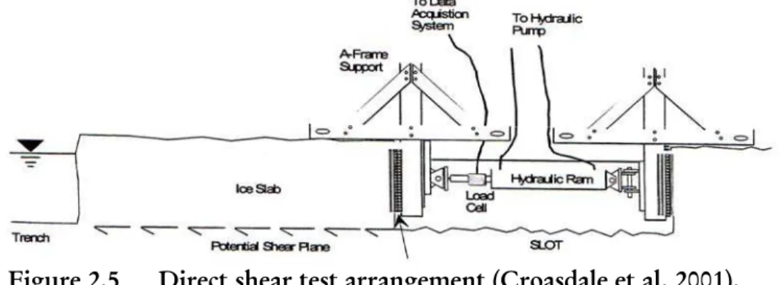
The direct shear test arrangement is shown in Figure 2.5. The test can be summarized as follows:

1. A rectangular slab from the refrozen layer of a ridge is isolated by trenching.

2. Load required to displace the slab horizontally is then measured while recording the corresponding displacement.

Figure 2.5 Direct shear test arrangement (Croasdale et al. 2001).

Figure 2.6 shows a typical load versus displacement plot for the direct shear test. The initial peak is a result of initial cohesive bond, which has to be overcome before the slab can be moved. On the other hand the long flat portion is believed to be related to residual frictional strength.

Figure 2.6 Typical load vs displacement in the direct shear test (Croasdale et al.2001) This test technique has been used successfully in four separate field projects, two in Canada and two in Russia (Croasdale et al., 2001). Croasdale et al. (2001) have reported the results of the eleven direct shear tests which have been conducted in Canada (1997) in the project conducted in Northumberland Strait. The maximum direct shear strength is defined as the peak load divided by the plan area of the block. The maximum value determined for the shear strength was 22.6 kPa and the average value was 14.1 kPa. The maximum value determined for the internal friction angle was 83o _{and the average value was 74}o_{. As the direct shear test is}

effectively measuring the shear strength of the rubble at the underside of the consolidated layer, subject to the maximum normal pressure in the keel, these results are a measure of the maximum strength of the keel. They may also be artificially high because of blocks that are anchored into the consolidated layer.

Pull Up Test

The test is used in order to investigate the presence of any bond between the consolidated layer and the rubble in the keel region, so it gives an indication of the cohesion in the upper part of the keel. It was first performed by Croasdale (1997). The test can be summarized as follows:

1. A rectangular slab through the consolidated layer has to be cut using a chainsaw.

2. These pre-cut rectangular slabs have to be pulled up vertically using a hydraulic ram and hinged beam apparatus; this will put the rubble directly below the consolidated layer in tension providing a pure cohesion value.

3. In the more recent tests in Russia, the apparatus consisted of a winch connected to a large ice screw in the ice block.

Croasdale et al. (2001) have reported the results of the eight pull up tests which were conducted in Canada (1997) in the project conducted in Northumberland Strait. The tensile bond strength is defined as the peak load divided by the block area. The maximum value measured for the tensile bond strength was 26 kPa and the average value was 17 kPa.

Punch Shear Test

The main advantage of the punch shear test is that the failure surfaces traverse the full depth of the ridge as in the passive failure mode of the ridge keel, therefore it helps to estimate large

scale average values of keel shear strength. On the other hand the other two tests examine the keel properties directly below the consolidated layer. As shown in Figure 2.7, in the punch shear test, a plug of the consolidated layer is cut through to the underlying rubble, and then a plug of the keel is failed downwards by applying a vertical load.

Figure 2.7 Configuration of the punch shear test (Croasdale et al. 2001)

Lepparanta and Hakala (1992) were the first researchers to try this test. Figure 2.8 shows typical load and displacement plots for punch shear tests. As in the direct shear test the strength reaches a maximum value after a very small displacement. The drop in load with displacement is not as obvious in the punch tests as in the direct shear tests, and this can be attributed to the progressive failure or to the high residual friction.

Figure 2.8 Typical load vs displacements, punch shear tests (Croasdale et al. 2001) The results of a punch test can be interpreted in three ways: pure friction, pure cohesion or a combination of both of them. Calculation of cohesion has been done usually as follows:

k d P h r w F c π 2 − = 2.9 Where Fp is the force on the platen, wd, the buoyant force, and r, the radius of platen. Fp has

been calculated by Meyerhof and Adams (1968) as follows:

(

φ

)

φ γ 1 0.025 25 tan 2 2 o k _u k e d p K d h d h w F ⎥⎦ ⎤ ⎢⎣ ⎡ _{+ −} + = 2.10 Rowe and Davis (1982) conducted a finite element analysis simulating the punch tests, and they concluded that Fp needs to be multiplied by a factor RΨ in order to account for the effect

of dilatancy of the rubble. Das and Singh (1995) had confirmed this conclusion and their confirmation was based on the fact that the Meyerhof equation underestimates the strength of a dense soil with a low hk/d ratio.

(

)

d h R =₁+ _0.0059φ −_0.135 k

ψ 2.11

Croasdale et al. (2001) have reported the results of the nine punch tests which have been conducted in Canada (1997) in the project conducted in Northumberland Strait. The punch shear strength is defined as the peak load divided by the product of the perimeter of the punch block and the keel depth. The maximum value measured for the punch shear strength was 12.8 kPa and the average value was 8.5 kPa. The maximum value determined for the internal friction angle was 69o _{and the average value was 57}o_{. The average punch shear strength is}

nearly half the average direct shear strength. This can be attributed to the variation of shear strength from a value of zero at the bottom of the keel to a maximum value just below the consolidated layer. These results confirm that the shear strength is dependent on normal pressure.

Heinonen and Määttänen (2000) have performed more recent punch shear tests. The strength parameters have been determined using an analytical limit load method. This method is based on the balance of internal and external work rate. Where the external work is the work done by the buoyancy force and the external force pushing the platen. And the internal work is the plastic work occurring at the shear lines between each block.

Figure 2.9 is a schematic showing a cross section of the keel failure planes and modes. They reported values of 2.3 kPa and 14o _{for the cohesion and the internal friction angle respectively.}

Figure 2.9 Ridge keel punch test (Heinonen and Määttänen 2000). Ridge Tests

An example of the recent approaches to explore the mechanical properties and the failure mechanisms of first year ice ridges is the in-situ tests conducted by Bonnemaire and Bjerkas. Bonnemaire and Bjerkas (2004) reported their observations of the 33 interactions between first year ridges and an instrumented lighthouse in brackish water. Based on their observations:

1. They concluded a relation between sail height and keel depth and how the keel depth grows with time.

2. They gave a detailed description of the failure modes and the sequence of their occurrence as summarized in Figure 2.10. And they stated that the crushing failure gives the highest loads during interaction with ice ridges.

Figure 2.10 Failure modes between ice ridges (lines) and cylindrical structures (top view) (Bonnemaire and Bjerkas 2004).

3. They stated that the most significant loads come from the consolidated layer and the upper part of the keel. And that there is a concentration of loads observed parallel to the drift direction as a result of crushing failure.

4. They found that the loads resulting from ridges are higher from those of the surrounding ice sheets by a factor ranging from 0.5 to 6, and that ridge loads increase with increasing sail height.

5. They reported that when ice ridge fails on a rubble wedge, loads seem to be concentrated on the two borders of the rubble wedges, usually 90± o _{to the drift}

direction.

2.5 First Year I ce Ridge Failure Modes and Load Calculation

When first year ice ridges interact with offshore structures, the main load components are from the partly consolidated keel and the refrozen upper part of the ridge (consolidated layer). Large forces are required in order to break both layers. The load due to the consolidated layer can be estimated using the methods for level ice as an approximation, however it is usual for the consolidated layer to be thicker than the surrounding level ice and the salinity, temperature and the porosity can be quite different. Most of the algorithms available for the failure of level ice do not account for the inhomogeneity that is common in consolidated layers.

Keel loads are subjected to greater uncertainties than the consolidated layer loads. Because of the similarities between keel rubble and soil (granular materials), much of the failure modeling has been based on the Mohr-Coulomb failure envelope for shear strength.

3 Comparison Betw een Measured Loads and existing Theories

In Chapter 2, many reasons have been stated to explain why the existing models can not be used efficiently to calculate the loads caused by the first year ice ridges interacting with the Confederation Bridge. Most of these above mentioned reasons are based on physical and mechanical properties of first year ice ridges. As a result, a detailed comparison between the recorded loads and the loads calculated using many of these existing theories needs to be done. This is essential to provide more evidence that the inefficiency of these models not only result from the poor knowledge of the mechanical and physical properties of ridges but also result from the incompatibility of these proposed models with the Confederation Bridge geometry. These comparisons use the ridge properties resulting from the detailed video and sonar data analysis that has been concerned about events of first year ice ridges interacting with the Confederation Bridge pier P31. These properties have been used to substitute in the existing load models for load calculation. Finally, the comparison will be between recorded loads and calculated loads for the same events.

3.1 Existing Load Models for Rubble Failure

3.1.1 Overview of Existing Analytical Keel Load Models – Local Failure

Theories for local ridge keel or rubble failure modes have been largely based on ideas based on soil mechanics techniques. This was based on the idea that both of the soil particles and the ice rubble are granular materials. Theories for local failure have been proposed by Dolgopolov et al. (1975), Prodanovic (1979), Mellor (1980), Hoikkanen (1984), Croasdale et al. (1994), Weaver (1994), Croasdale (1980), Croasdale and Cammaert (1993) and Karna (2001). Each theory will be discussed briefly in turn.

Dolgopolov et al. (1975) developed a theory based on some observations from experiments. The horizontal load is given by:

⎟⎟ ⎠ ⎞ ⎜⎜ ⎝ ⎛ + =h D q h c F k e e k k η η γ 2 2 2 3.1

Where hk is the keel depth, De is the effective structure width, γe is the effective buoyant

density, c is the apparent cohesion, and η is the passive pressure coefficient, which is given by ⎟ ⎠ ⎞ ⎜ ⎝ ⎛ ₊ ≈ − + = 2 45 tan sin 1 sin 1 0 φ φ φ η 3.2

Equation 3.1 assumes local failure of rubble. The local failure is based on the depth of the keel; a deeper keel will cause a higher load Fk. It is based on Mohr-Coulomb material behaviour

any slip planes. The shape factor q is a factor that accounts for the increased keel depth caused by the interaction e k D h q 3 2 1+ = 3.3

The effective buoyancy γe was not used in the original paper, as Dolgopolov used the

buoyancy of the ice. But generally, the effective buoyancy has been used as it accounts for the effect of the void ratio n

(

_{w i}

) (

g n

e = ρ −ρ 1−

)

γ 3.4 where ρw and ρi are the densities of sea water and ice, respectively. Dolgopolov suggests, as a

result of his tests, that the accumulation of rubble against the structure should take the form 2 e k k D h h = ′ + 3.5 where hk` is the depth at a certain penetration level. Because the method is for local passive

failure, it will be conservative for a ridge with limited width where a global plug failure can occur before the maximum depth of the ridge has been penetrated by the structure. Equation 3.5 leads to some concern as, for a very wide structure, the surcharge will be very large. As a result the Dolgopolov expression for local keel failure should not be used for wide structures. Prodanovic (1979) developed load methods (an upper bound theory) for first year ridges based on limit equilibrium models, plasticity theory and Mohr-Coulomb behavior.

⎥ ⎦ ⎤ ⎢ ⎣ ⎡ ⎟⎟ ⎠ ⎞ ⎜⎜ ⎝ ⎛ + + = e k e k k e p k D h b D h a h D F σ 1 1 3.6 ⎟ ⎠ ⎞ ⎜ ⎝ ⎛ ₊ = 2 45 tan 2 φ σ o p c 3.7

(

)

[

o

]

a=0.891+1.82tanφ−17 3.8

[

1 2.01tan( 8 )

]

31 . 0 o b= + φ− 3.9 Where σp is the plane strain compressive strength of the ice rubble, c is the cohesion and φ is

the internal friction angle. a and b are coefficients that are based on minimizing energy and depend on the effective internal friction. This method is recommended by the American Petroleum Institute (API, 1994).

Mellor (1980) predicted the brash ice forces acting on ships in which two passive wedges were assumed to develop and it was shown that the same method can be used for ridge keels. He proposed that the rubble in the keel and the sail, slip along planes that make a constant angle with the horizontal. The horizontal force due to the sail Fh,s is given by:

(

)

i s e s

e s

h D n gh Dc h

F_, =0.5 η2 1− ρ 2 +2 η 3.10 where hs is the sail height. The horizontal force due to the keel Fh,k is given by

(

)(

_{w i}

)

_{k e k} e

k

h D n gh D c h

F_, =0.5 η2 1− ρ −ρ 2 +2 η 3.11 The total horizontal force due to the sail and the keel is given by the simple sum of these two components: Fh = Fh,s+ Fh,k This method is also recommended by the American Petroleum

Institute (API, 1994).

Hoikkanen (1984) developed a load model that predicts the maximum horizontal load on a structure due to the sail and keel portions. This model was based on an assumption of a linear variation of pressure with depth. The pressure due to the sail is assumed to vary linearly between P1 at the top and P2 at the bottom of the sail, while the pressure due to the keel varies

linearly between P3 at the top and P4 at the bottom of the keel. The pressures are given by:

s s c P₁ =2 η 3.12 ) 1 ( 2 2 c gh n P = _s η_s +η_sρ_{i s} − 3.13

(

n gh c P₃ =2 _k η_k +η_kρ_{i s} 1−

)

3.14

(

)

₍

(

₎

)

_⎟⎟ ⎠ ⎞ ⎜⎜ ⎝ ⎛ ⎭ ⎬ ⎫ ⎩ ⎨ ⎧ − − − − − + = s i k i w s i k k k h n g gh n n gh c P 1 ] 1 [ min 1 2 4 _ρ ρ ρ ρ η η 3.15

Where cs and ηs are the cohesion and the passive pressure coefficient for the ridge sail, and ck

and ηk are the cohesion and passive pressure coefficient for the ridge keel. The force due to the

sail:

(

)

_⎥ ⎦ ⎤ ⎢ ⎣ ⎡ ⎟ ⎠ ⎞ ⎜ ⎝ ⎛ ₊ − + ⎟⎟ ⎠ ⎞ ⎜⎜ ⎝ ⎛ + = _{s s s} s h h P P Dh P P F α β φ cot 3 3 2 5 . 0 tan tan 1 1 2 2 2 1 , 3.16

and the force due to the keel:

(

)

_⎥ ⎦ ⎤ ⎢ ⎣ ⎡ ⎟ ⎠ ⎞ ⎜ ⎝ ⎛ ₊ − + ⎟⎟ ⎠ ⎞ ⎜⎜ ⎝ ⎛ + = _{k k k} k h h P P Dh P P F α β φ cot 3 2 3 5 . 0 tan tan 1 3 4 2 4 3 , 3.17

where β is half of the leading angle of the rubble bow formed in front of the structure and can be assumed to be 45o_. α

s and αk represent the slope angles of the structure interacting with the

sail and the keel. This method is somehow unrealistic, as the keel load is strongly influenced by the sail height through the pressures P3 and P4. The total horizontal force due to the sail

and the keel is given by the simple sum of these two components: Fh = Fh,s+ Fh,k.

Croasdale (1994) developed a wedge failure theory. This theory assumes the keel to fail locally in a wedge limited by three planes. One plane is inclined at 45o _{and starts from the}

intersection of the keel and the consolidated layer and extends down through the rubble, and the other two planes are vertical, bounding the sides of the wedge.

(

2

)

2 _{k e k}

e

h c h D h

F = + 3.18 where ce is the effective cohesive strength of the rubble. This can be obtained from the keel

properties as: c h c k _e e = γ tanφ+ 2 3.19 Weaver (1994) proposed two equations for frictional and cohesive materials. The equation for the maximum frictional resistance can be expressed as follows:

2 2 5 . 1 _eγ_{e k}η h D h F = 3.20 and the equation for cohesive resistance is:

k e k e h cDh h D F _⎟⎟ ⎠ ⎞ ⎜⎜ ⎝ ⎛ + =5.14 0.32 0.12 3.21

3.1.2 Overview of Existing Analytical Keel Load Models – Global Failure

Some of the theories that have been proposed treat the failure of the ridge in a global sense. These include Croasdale (1980) and Croasdale and Cammaert (1993).

Croasdale (1980) proposed a model that was based on a cylindrical structure and accounts for shear stresses only on the sides of the plug along two vertical planes parallel to the structure (see Figure 3.1).

Figure 3.1 Plug failure planes in a ridge keel Croasdale’s equation can be written as:

(

ρ ρ

)

tanφ 3 2 2 g h W F_k = _{R k w} − _i 3.22 3-4

where WR is the width of the ridge. According to this equation, the force does not depend on

the diameter of the structure or the cohesion of the ice rubble.

Croasdale and Cammaert (1993) modified the original plug failure model in order to account for ridges contacting structures at angles other than 90o _{as well as the possibility of}

non-parallel failure planes (ω). A third failure plane was added under the consolidated layer and was assumed to act simultaneously with the two side planes. The force due to the plug failure was determined as:

φ γ ω ω 0.39 0.2 tan tan cos 26 . 0 e R e k p k e R K D W h K h D W F ⎟ ⎠ ⎞ ⎜ ⎝ ⎛ _{+ +} = 3.23

Kärnä et al. (2001) developed a passive pressure failure model for the ridge keel. The cross section considered during the development of this model is shown in Figure 3.2. This figure illustrates the geometry of the ice ridge during the initial penetration condition.

Figure 3.2 Cross section and parameters of a first year ridge (Karnä and Nykänen 2004)

The model simulates the ridge penetration as a sequence of discrete failure events and searches at every penetration interval for the path of least resistance, similar to the GPF model of Croasdale et al. (1995). Figure 3.3 clarifies the failure mechanism showing the three assumed failure planes:

a) Sloping down from the structure, just below the consolidated layer to the base of the keel (AA`E`E).

b) Failure plane that originates from the side of the structure (AEHG). c) Failure plane that originates from the side of the structure (A`E`H`G`).

Figure 3.3 Failure mechanism with an inclined slip plane and two vertical slip planes (Karnä et al. 2001).

The amount of penetration and the internal strength properties of the ridge decide whether the individual failure event can be characterized either as a local failure or as a plug failure (Brown et al., 1996, Croasdale, 1999). The model considers the evolution of the ice ridge by redistributing the failed ice rubble below and behind the original keel profile. As a result, this model considers the surcharge effect that occurs while the keel height increases during the interaction.

The horizontal load component that arises due to the frictional resistance at the slip plane AEE`A` can be calculated using the following formula:

(

)

(

) (

s s e i w gD A n P δ α α ρ δ

)

φ ρ ρ ρ φ = − − ₊ +₊ cos + cos sin ) )( 1 ( 1 3.24 Where:

A: Area of the cross section,

ρ: Inclination angle of the slip plane

δ : Friction angle between the rubble and the structure

s

α : Inclination of the structure wall

The frictional resistance provided by the vertical slip planes can be calculated as follows:

ρ φ φ φ 2 2 tan cos 2 R P = 3.25 Where R2φis the resultant of the normal pressures acting on the vertical slip surface AGFBHE

3.26

∫

= A kzdA R_2φ γ

The cohesion resistance provided by the inclined slip plane can be calculated as follows:

ρ

cot

1C ceDehe

P = 3.27 To evaluate the cohesion forces P2c acting at the vertical slip planes:

ρ cos 2 ₂ 2 c A P_c = 3.28 3-6

)

As c2 is the cohesion below the shear key region

The equations 3.24, 3.25, 3.27 and 3.28 are the peak values of the various frictional and cohesion force components. Since these peak values may not occur simultaneously so the formulae are derived separately. As a result the combination of these load components can not be done as a direct sum, since this will be an overestimation of the keel load component. Therefore the total keel load component is:

(

)

(

2 2 1 2 2 1 C C K P P P P F = φ + φ + + 3.29

Equation 3.29 estimates the keel load component for any penetration distance and for any slip angle.

Weaver [Croasdale et al. (1995)] developed the General Passive Failure Model (GPF Model) based on classical soil mechanics theory for a compressible linear Mohr-Coulomb material. The model searches for the lowest load at each penetration level. The model resolves all of the forces acting on the failure wedge and determines the resultant horizontal force for a given (the vertical inclination of the primary failure plane). The model takes into account, inertial effects, deviation of the failure planes from normal, rubble accumulation in front of the pier and the confining pressure on the failure planes. The user inputs the structure and the ridge dimensions as well as the strength parameters of the rubble. The model then searches for the critical plane geometry (critical β), by modifying θ in the Figure 3.4, the lowest load for each penetration level can be estimated.

Figure 3.4 General passive failure model (Croasdale 1999).

The model takes non-vertical structure wall friction and the formation of surcharge in front of the pier during penetration into consideration. The factor which accounts for surcharge varies from 0 to 1. The inertia is modeled by a hydrodynamic added mass factor. This factor varies from 0 to 2. An upper bound solution to the ice load maybe taken as the lower of the following two limit cases:

Where ω is the angle of divergence of the vertical walls of the failure wedge from the direction of the ice movement.

Vershinin et al. (2001): developed a model based on the Mohr-Coulomb failure envelope for a material in confined conditions considering both the cohesion and the internal angle of friction of the ice rubble forming the ridge keel. This method proposes that a keel of a pressure ridge interacting with a finite width structure fails along a shear wedge formed by ice fragments in either of two modes: by elevation sliding, or by plane sliding. In calculating the load for zones of plane sliding, the structure slope is considered. For wide keel ridges, the influence of the sea floor and the bottom of the consolidated layer are considered, leading to additional rubble compression, which may change the dimension of the elevation and plane zones and, subsequently increase loads.

Figure 3.5 shows a cross-section schematic of the assumed failure pattern and Figure 3.6 gives a plan view of the failure.

Figure 3.5 Cross-section sliding scheme. Figure 3.6 Plan of sliding scheme

(Vershinin et al. 2001). In the absence of sea bed effects, the loads are as follows:

The force in the zone of elevation sliding for a cylindrical structure with diameter D is calculated as follows:

(

h K C K

)

(

h h

)

D K K

(

h h D K

P_{elev D b k p p k plane} b D p . _{k plane}. 2 . . . . . 2 . . . 3 2 2 3 + − − − = γ γ

)

3.30

Kp is the passive pressure coefficient and is calculated as follows:

(

)

(

)

₍

(

)

₎

2 2 2 sin sin sin sin 1 sin sin sin ⎥ ⎦ ⎤ ⎢ ⎣ ⎡ − + + − + = α δ α ϕ δ ϕ δ α α ϕ α P K 3.31

And K3D is an empirical factor that accounts for an increase in keel depth due to the

interaction (see Dolgopolov et al, 1975) and is equal to:

( )

_{( )}

h D h h K _D k . 3 . 2 1 3 = + 3.32 Where: α : Cone angle.

δ : Friction angle of the ice fragments with the surface of the structure. D(h): The structure diameter on depth level h.

hplane: The boundary depth between plane and elevation sliding zone.

The force in the zone of elevation sliding for a cylindrical structure with diameter D is calculated as follows:

(

h K C K

)

(

h h

)

D K K

(

h h D K P b D P _{k plane} plane k p p k b D plane . . 2 . . . . . 2 . . 3 2 2 . 3 + − − − = γ γ

)

3.33

Including the effects of the sea-bed and the consolidated layer, the only change in the keel-structure interaction is that the rubble pressure in the lower part of the keel is not equal to zero.

Assuming that the keel internal pressure does not change after the cutoff of the lower portion of the keel during the interaction, a lower bound of the pressure at the bottom of sea level can be estimated. The upper bound of the pressure at the bottom of the sea level is the compressive strength of the ice, as the rubble pressure can not exceed it.

Surkov (2004) has developed a method to estimate first year ridge loads on cylindrical supports based on laboratory and field experiments. He also presented a comparison between the various methods of calculation of first year ridge loads. Surkov (2004) used the following approach to calculating the loads of first year ridges on cylindrical supports:

FH=FC+FHK 3.34

Where:

FC: The load due to the consolidated layer.

FHK: The load due to the keel.

The load due to the consolidated layer is determined by the well known classical expression developed by K.N. Korzhavin, which is as follows:

FC=Ik1k2σcDhi 3.35

Where:

I: Indentation coefficient, k1: Shape factor,

k2: Ideal contact coefficient

The ideal contact coefficient k2 varies from a value of 0.3 to a value of 1, and the indentation

coefficient depends on the ratio of the support width to ice thickness (D/hi), and it is

( )

0.22 77 . 2 − = h D I 3.36 The load due to the keel is estimated using an equation similar to equation 3.35 as follows:

* k H HK Jim DH F = σ 3.37 Where:

J: The indentation coefficient,

i: The shape factor and is taken as unity.

m: The ideal contact coefficient for keel-support interaction and is taken as unity.

σH: Keel uniaxial compressive strength.

*

k

H : The keel thickness (equal to its draft Hk minus the thickness of the consolidated layer)

Because of the uncertainty that is present in the process of expressing the keel crushing strength σH in terms of Coulomb-Mohr parameters, Surkov (2000) expressed σH in terms of

the crushing strength of the consolidated layer σc as follows:

) 100 . ( 255 . 0 1 n n c H = − σ σ

where n is the porosity of the keel 3.38 Dolgopolov et al., (1975), Prodanovic, (1979) and Coon et al., (1984) had presented three methods in order to calculate the indentation factor (J) [Surkov, (2004)]. But due to a comparison presented by Surkov (2004), it was determined that the equation developed by Dolgopolov et al., (1975) gave the most realistic values and it is as follows:

D H J k . 3 * . 2 1+ = 3.39 The model of Surkov (2004) predicts the lowest loads as follows:

FHk=khFi 3.40

Where:

Fi: The load exerted by the level ice on the support.

kh: Ratio between load exerted by the ridge keel and that exerted by the level ice on the

support.

And kh was estimated by Surkov (2004) as follows:

⎥⎦ ⎤ ⎢⎣ ⎡ ⎟ ⎠ ⎞ ⎜ ⎝ ⎛ − = i h D_h k exp 1.35 0.34ln 3.41 3-10

Surkov (2004) made a comparison between the ice loads on supports estimated by the models of different authors. He found that the lowest loads estimated were by his method. Figure 3.7 shows this comparison for structures with D≤10m while Figure 3.8 is for structures with width D≤100m.

Figure 3.7 D 10m, ≤ Figure 3.8 D≤ 100m Load due to ice ridge vs support diameter, Surkov, 2004).

This comparison showed that the model of Prodanovic (1979) gives unrealistic values, and that the model of Coon et al. (1984) also gives high values. On the other hand this comparison showed that the models of Dolgopolov et al. (1975) and Määttänen (1984) gave results close to the lowest loads predicted by Surkov’s method.

Nevel (2001) realized that the current theories that are used in the determination of first year ridges loads and failure modes are not suitable for conical structures. He derived equations that can predict the vertical forces, horizontal forces and overturning moments resulting from the rubble from both the keel and the sail of a first year pressure ridge, interacting with downward breaking cone structures. The structure he used in his derivation is composed of a number of cone sections that end with a vertical neck. He proposed that the vertical stresses acting on the keel and sail are the buoyancy and gravity stresses; on the other hand the horizontal stresses in the rubble are determined from the Mohr-Coulomb shear failure criteria. By integrating the horizontal stresses in the rubble over the area of the structure, projected in the vertical plane, the horizontal force on the structure was obtained. Similarly the vertical force on the structure was obtained by integrating the vertical stress in the keel over the area of the structure projected onto a horizontal plane.

Nevel (2001) calculated the keel horizontal force on a cone section to be:

FX = D[A(T-S)+B](R1+R2)-AD2(R1+2R2)/3 3.42

(

)(

)

_⎟⎟ ⎠ ⎞ ⎜⎜ ⎝ ⎛ − + − − = ϕ ϕ γ γ sin 1 sin 1 1 n A _{W I} 3.43 2 1 sin 1 sin 1 2 _⎟⎟ ⎠ ⎞ ⎜⎜ ⎝ ⎛ − + = ϕ ϕ C B 3.44

Where: C: Cohesion

ϕ: Internal friction angle D: Height of the cone section, T: Depth of the keel,

n: Porosity of keel.

S: Distance from the water surface to the cone section. R1: Large radius of the cone’s section.

R2: Small radius of the cone’s section.

ρw: Weight of water per volume,

ρI: Weight of ice per volume.

The vertical force on a cone section is calculated as follows:

Fz= π E(T-S)(R1-R2)(R1+R2)/2-πED(R1-R2)(R1+2R2)/6 3.45

Where:

E=(ρW- ρI)(1-n) 3.46

The keel horizontal force on neck of a cone is calculated as follows:

FX=2RD[A(T-S-D/2)+B] 3.47

The drag layer’s horizontal force on a cone:

FX=G(T-S)[A(T-S)+2B] 3.48

The sail horizontal force on a cone section:

FX=JV2(r1+2r2)/3+BV(r1+r2) 3.49 Where:

(

)

_⎟⎟ ⎠ ⎞ ⎜⎜ ⎝ ⎛ − + − = ϕ ϕ γ sin 1 sin 1 1 n J _I 3.50 V: Height of the sail,

r1: Large radius at the top of the sail.

r2: Small radius at the water line.

So Nevel’s method estimated forces and moments acting on all conical sections and the neck, in addition it estimated the force due to the drag layer adjacent to the cone. All the forces are to be added together in order to get the total.

Cammaert et al. (1993) developed the cross-over model which between the Dolgopolov passive failure model (Dolgopolov et al, 1975) and the Croasdale plug model (Croasdale and Cammaert, 1993). This model recognizes that ridge indentation is a continuous process and that the plug failure load is reduced as the ridge is indented. The analysis proceeds by stepping through the ridge in convenient increments, and determining the loads by the two methods at each location. The model is important because local and global failures are dependent on different parameters. For the analysis, the actual keel depth at each location is used for the Dolgopolov model, while the residual cross sectional area is determined for the use of the plug model. The minimum of the two loads is then selected as the ridge keel load for the structure at that position of the ridge.

Figure 3.9 shows that in many cases, the maximum value of neither failure model will be the ultimate load during a keel interaction. The local failure load will increase with the depth to maximum near the center of the keel. The global load will be a maximum at the beginning of the interaction and will decrease as less keel area remains in the interaction.

The ultimate keel load will occur midway through the keel when a plug failure will require less load than a local failure. This method is less conservative than either the Dolgopolov load based on maximum keel depth or the Croasdale plug load based on full cross sectional area.

Figure 3.9 Cross over model showing progression of failure loads (Lemée and Brown 2002).

3.2 Modified Consolidated Layer Flexure Load Model Used in the Comparison

Observations from the video monitoring system show that there is a significant upward thrust by the rubble from the keel on the underside of the consolidated layer. This will reduce the force required to cause a flexural failure. Based on his detailed video analysis, Lemee (2003) made some modifications to the flexural failure equation of Croasdale et al. (1994). The observations indicate that the two rubble terms for lifting the rubble on top of the consolidated layer and the force required to push the consolidated layer through the rubble

will be greatly reduced and in some cases eliminated. So the modified expression for the horizontal force caused by the consolidated layer is (Lemee, 2003):

T R P B C H H H H F = + + + 2 3.51 Where the expressions for HB, HT, HP and HR are presented in Croasdale et al., 1994.

HB is the breaking force, and the expression used is:

( )D e c e B B H D I D H / 4 2 2 ⎥ ⎦ ⎤ ⎢ ⎣ ⎡ ⎟⎟ ⎠ ⎞ ⎜⎜ ⎝ ⎛ + = π 3.52 Ic is the characteristic length and is given as:

(

)

[

(

_{3 2} 0.25 1 12 / ρ −ν = Eh g I_{c w}

]

)

3.53 ( )

(

₍

)

₎

25 . 0 5 2 sin cos cos sin 68 . 0 _⎟⎟ ⎠ ⎞ ⎜⎜ ⎝ ⎛ − + = E gh D H w e f s s D B ρ σ α µ α α µ α 3.54

where h is the ice thickness, E is the elastic modulus, µs is the friction coefficient of ice with

structure, α is the structure slope angle, σf is the flexure strength and ν is Poisson ratio.

HT is the force for the turning of blocks at the top of cone and the expression used is:

(

[

φ φ µ ϕ

ρ cos / sin cos 5 . 1 2 s e i T h gD H = −

)

]

3.55 HP is the force necessary to push the consolidated layer through the ice rubble and the

expression used is:

(

γ

)(

θ α

) (

θ

)

ρ

µ 1 1 tan /tan 2 1/2tan

2 − −

=D h g

H_{P e r i i} 3.56

where µi is the ice to ice friction coefficient, hr is the rubble height and θ is the angle the

rubble surface makes with the horizontal.

HR is the additional force necessary to push the ice blocks up the slope through the ice rubble

and the expression used is:

[

(

1/cosα µ_ssinα

]

)

e R D P H = − 3.57 where: 3-14

(

) ( )

(

)(

)

(

) ( )

(

)(

)

[

]

(

α µ α α

)

ρ α θ α α γ ρ µ µ α θ α θ α γ ρ µ µ µ sin / cos sin tan / tan 1 tan / 1 cos 1 5 . 0 tan / tan 1 tan / 1 tan / 1 sin 1 5 . 0 2 2 s i r r i s i r i s i i g h h h g h g P + + − − + + − − − + = 3.58 3.3 Model Comparisons 3.3.1 Croasdale ( 1998)

Croasdale (1998) presented a comparison of many of the earlier models. The ridge used in his comparison was a 20 m deep triangular keel acting on two vertical structures of 10m and 100m width, respectively, assuming either pure cohesional strength (of 25 kpa) or pure frictional strength (φ=45o_{). The keel slope angles are assumed to be 35}o_{. The results are}

summarized in Table 3.1.

Table 3-1 Comparison of Methods for Keel Loads [Croasdale (1998)] Method Structure Width (m) Rubble Friction Angle (o₎ Rubble Cohesion (kpa) Calculated Load (MN) Dolgopolov 10 45 - 27.2 Mellor 10 45 - 39.8 Croasdale 10 45 - 13.3 Dolgopolov 10 - 25 28 Mellor 10 - 25 12 Dolgopolov 100 45 - 132 Mellor 100 45 - 398 Croasdale 100 45 - 65 Dolgopolov 100 - 25 136 Mellor 100 - 25 120

This comparison showed differences in loads for the same case by up to a factor of six. This clearly suggests that some of these methods are unsatisfactory, and new models have to be developed.

3.3.2 Summary of the Events Used in the Comparison

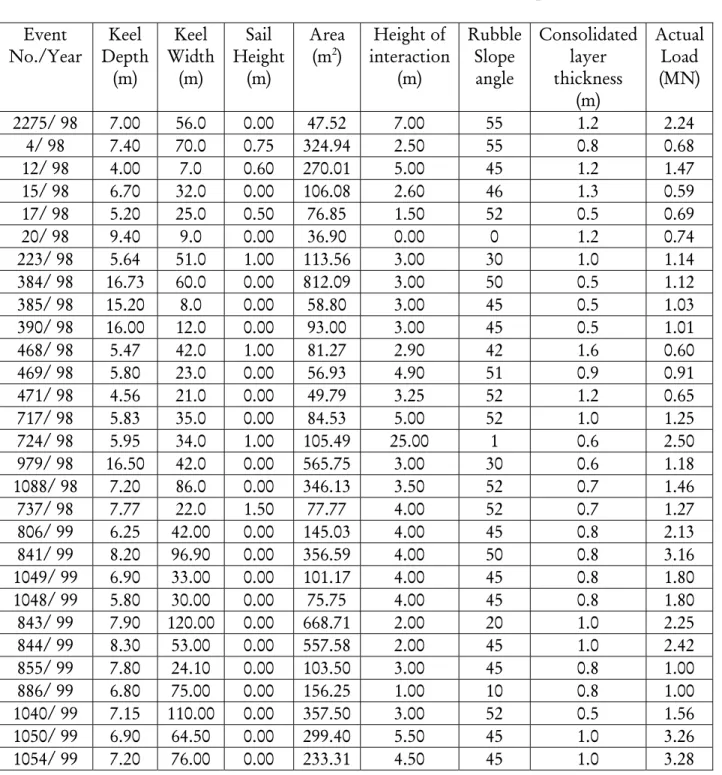
In order to further test the existing models a series of analyses were undertaken using observed ridges for the Confederation Bridge Ice force Monitoring programme. A total of 50 ridges for which good sonar data was available and for which measured loads were also available, were selected. The relevant information for these 50 ridges is given in Table 3.2.

Table 3-2 Summary of the events used in the comparison Event No./Year Keel Depth (m) Keel Width (m) Sail Height (m) Area (m2₎ Height of interaction (m) Rubble Slope angle Consolidated layer thickness (m) Actual Load (MN) 2275/ 98 7.00 56.0 0.00 47.52 7.00 55 1.2 2.24 4/ 98 7.40 70.0 0.75 324.94 2.50 55 0.8 0.68 12/ 98 4.00 7.0 0.60 270.01 5.00 45 1.2 1.47 15/ 98 6.70 32.0 0.00 106.08 2.60 46 1.3 0.59 17/ 98 5.20 25.0 0.50 76.85 1.50 52 0.5 0.69 20/ 98 9.40 9.0 0.00 36.90 0.00 0 1.2 0.74 223/ 98 5.64 51.0 1.00 113.56 3.00 30 1.0 1.14 384/ 98 16.73 60.0 0.00 812.09 3.00 50 0.5 1.12 385/ 98 15.20 8.0 0.00 58.80 3.00 45 0.5 1.03 390/ 98 16.00 12.0 0.00 93.00 3.00 45 0.5 1.01 468/ 98 5.47 42.0 1.00 81.27 2.90 42 1.6 0.60 469/ 98 5.80 23.0 0.00 56.93 4.90 51 0.9 0.91 471/ 98 4.56 21.0 0.00 49.79 3.25 52 1.2 0.65 717/ 98 5.83 35.0 0.00 84.53 5.00 52 1.0 1.25 724/ 98 5.95 34.0 1.00 105.49 25.00 1 0.6 2.50 979/ 98 16.50 42.0 0.00 565.75 3.00 30 0.6 1.18 1088/ 98 7.20 86.0 0.00 346.13 3.50 52 0.7 1.46 737/ 98 7.77 22.0 1.50 77.77 4.00 52 0.7 1.27 806/ 99 6.25 42.00 0.00 145.03 4.00 45 0.8 2.13 841/ 99 8.20 96.90 0.00 356.59 4.00 50 0.8 3.16 1049/ 99 6.90 33.00 0.00 101.17 4.00 45 0.8 1.80 1048/ 99 5.80 30.00 0.00 75.75 4.00 45 0.8 1.80 843/ 99 7.90 120.00 0.00 668.71 2.00 20 1.0 2.25 844/ 99 8.30 53.00 0.00 557.58 2.00 45 1.0 2.42 855/ 99 7.80 24.10 0.00 103.50 3.00 45 0.8 1.00 886/ 99 6.80 75.00 0.00 156.25 1.00 10 0.8 1.00 1040/ 99 7.15 110.00 0.00 357.50 3.00 52 0.5 1.56 1050/ 99 6.90 64.50 0.00 299.40 5.50 45 1.0 3.26 1054/ 99 7.20 76.00 0.00 233.31 4.50 45 1.0 3.28 3-16

Event No./Year Keel Depth (m) Keel Width (m) Sail Height (m) Area (m2₎ Height of interaction (m) Rubble Slope angle Consolidated layer thickness (m) Actual Load (MN) 1067/ 99 6.00 54.00 0.00 180.28 2.00 30 0.8 2.53 1181/ 99 7.48 75.00 0.00 311.16 1.40 0 1.3 1.04 1182/ 99 6.20 25.50 0.00 62.48 4.25 74 1.3 1.07 1322/ 99 6.18 77.00 0.00 218.76 2.00 45 0.5 2.34 1324/ 99 5.40 57.00 0.00 131.81 3.00 52 0.8 1.49 1334/ 99 9.30 49.50 0.00 245.73 3.00 55 1.0 1.14 835/ 99 4.83 54.00 0.00 108.81 2.00 25 0.8 2.80 837/ 99 7.30 48.00 0.00 163.20 1.00 21 0.5 2.10 840/ 99 8.30 76.00 0.00 277.40 3.00 30 0.9 2.30 852/ 99 7.00 40.00 0.00 151.87 3.00 20 0.7 1.60 475/ 2000 6.40 52.00 0.00 140.67 3.00 45 1.0 1.56 1005/2000 9.00 42.00 0.00 174.49 5.00 45 0.8 3.36 1007/2000 6.60 34.00 0.00 117.90 5.00 45 0.8 2.49 487/2000 5.90 30.00 0.00 82.60 6.00 45 1.0 2.75 390 5.30 52.00 1.90 151.58 2.80 27 1.0 1.12 533 6.30 19.00 1.00 51.35 4.00 28 0.8 1.22 3.3.3 Comparison Procedure

The comparison procedure can be summarized in the following:

• A detailed video and sonar data analysis has been carried out to establish the actual geometric and physical properties of the ridges for which their interaction loads with pier P31 have been recorded.

• The geometric and physical properties estimated in step 1 have been used to calculate the loads expected using existing first year ridges’ load models. These load models have been presented in section 3.1.

• Several combinations of the values of c and ϕ have been used in order to investigate their influence on the load models and how the results for the above mentioned load models depend on the values for c and ϕ.

• The recorded loads and the calculated loads have been compared to assess the consistency of the existing load models with the loads recorded during the Confederation Bridge Monitoring Program.

• The relation between the calculated load of each load model and the recorded load has been plotted. Also the percentage by which each load model over predicts the recorded load has been calculated to determine to what extent each load model differs from the recorded load.

3.3.4 Comparison Results

Figures 3.10 to 3.19 present the relation between the calculated loads of each load model and the recorded load. For Figures 3.10 to 3.19 the values of c and ϕ have been taken as 5 kPa and 30o _{respectively. It is clear from the figures that there is no consistency between the recorded}

loads from the Confederation Bridge Monitoring Program and the calculated loads. Subsequently, the relation between the recorded and the calculated loads is considered to be very weak.

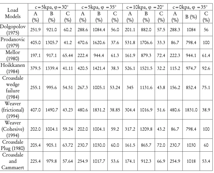
Table 3.3 shows the average and the maximum percentage by which each load model over predicts the recorded load. Also it presents the average percentage that the consolidated layer load represents in all the load models to estimate the weight of the consolidated layer load in the calculated loads.

Table 3-3 Difference between the calculated and the recorded loads

c=5kpa, ϕ=30o _{c=5kpa, ϕ =35}o _{c=10kpa, ϕ =20}o _{c=0kpa, ϕ =35}o

Load Models A (%) B (%) C (%) A (%) B (%) C (%) A (%) B (%) C (%) A (%) B (%) C (%) Dolgopolov (1975) 251.9 921.0 60.2 288.6 1084.4 56.0 201.1 882.0 57.5 288.3 1084 56 Prodanovic (1979) 405.0 1305.7 41.2 470.6 1620.6 37.6 531.8 1706.6 33.3 86.7 798.4 100 Mellor (1980) 197.1 917.1 65.44 222.4 944.4 61.3 161.9 879.3 72.4 222.3 944.1 61.4 Hoikkanen (1984) 379.5 1339.4 41.11 420.5 1421.4 38.3 526.1 1521.5 32.2 115.2 974.7 92.6 Croasdale wedge failure (1984) 255.1 995.6 54.51 267.3 1005.1 53.24 345 1131.6 43.8 156.2 852.4 75.1 Weaver (frictional) (1994) 407.0 1490.7 43.23 480.6 1831.2 38.85 304.4 1016.9 51.6 480.6 1831.0 38.9 Weaver (Cohesive) (1994) 202.0 1004.1 59.24 202.0 1004.1 59.2 317.2 1209.8 43.2 86.7 798.4 100 Croasdale Plug (1980) 205.4 905.1 63.72 230.7 1030.0 60.0 161.5 865.7 72.0 230.7 1030 60 Croasdale and Cammaert 225.4 979.8 57.64 254.9 1017.7 53.6 174.1 912.3 66.9 254.9 1018 53.4 3-18