Analyzing and minimizing capacity fade through optimal model-based control: theory and experimental validation

The MIT Faculty has made this article openly available. Please share

how this access benefits you. Your story matters.

Citation Pathak, Manan, et al., "Analyzing and minimizing capacity fade through optimal model-based control: theory and

experimental validation." ECS transactions 75 (2016): no. 23 doi 10.1149/07523.0051ECST ©2016 Author(s)

As Published 10.1149/07523.0051ECST

Publisher The Electrochemical Society

Version Final published version

Citable link https://hdl.handle.net/1721.1/124508

Terms of Use Article is made available in accordance with the publisher's policy and may be subject to US copyright law. Please refer to the publisher's site for terms of use.

Analyzing and Minimizing Capacity Fade through Optimal Model-based Control – Theory and Experimental Validation

Manan Pathak,1 Dayaram Sonawane,2 Shriram Santhanagopalan,3 Richard D. Braatz,4 and Venkat R. Subramanian1,5

1

University of Washington Seattle, WA

2

College of Engineering, Pune, MH, India

3

National Renewable Energy Laboratory, Golden, CO

4

Massachusetts Institute of Technology, Cambridge, MA

5

Pacific Northwest National Laboratory, Richland, WA

Abstract

In order to significantly expand the BEV market, and to increase the use of lithium-ion batteries in electric grids, there is a need to develop optimal charging strategies to utilize the batteries more efficiently and enable longer life. Advanced battery management systems that can calculate and implement such strategies in real time are expected to play a critical role for this purpose. This article investigates different approaches for determining model-based optimal charging profiles for batteries, and experimentally validates the gain obtained using such profiles. Optimal profiles that maximize the cycle life of the cells are implemented on 16 Ah NMC cells for 30 minutes of charge followed by 5C discharge, and the cycle life is compared to a standard 2C CC-CV charge and 5C discharge. An improvement of more than 100% in cycle life is observed experimentally, for our test conditions on this cell design. This study is the first to experimentally demonstrate that the improved extra knowledge obtained by sophisticated physics-based models results in significant improvements in battery performance when employed in a real time control algorithm.

Introduction

With the increase in global warming, societal pressure is increasing emphasis on renewable and clean energy. Alternative energy sources are aggressively being investigated and developed. Norway has become the first country to ban fuel-based cars by 2025, pushing the

Department of Energy and the recent announcement of a $50M grant for the Battery500 initiative,1 the U.S. government is also encouraging the commercialization of EVs. Apart from the automobile industry, the economics of distributed energy resources for power generation are also becoming increasingly favorable. The efficient use of these systems composed of intermittent renewable sources, such as wind and solar energy, depends critically on the efficiency of energy storage technologies. Because of its high power and energy density compared to other battery chemistries, the lithium-ion battery is one of the front-runners for energy storage alternatives. With the prices of the batteries reducing each year, the market for Li-ion batteries is bigger than ever.2

The performance of a Li-ion battery depends on the conditions of use, along with the state of internal variables. Thermal runaway, capacity fade, underutilization, and loss in power density are some of the main concerns with Li-ion batteries. Active research is being pursued to mitigate these issues. Various system-level strategies are being investigated to increase the efficiency of the existing and emerging systems. At the system level, battery management systems (BMS) play a critical role in managing the battery.

Most of the currently available BMS use empirical or lookup table-based models to predict the internal states of the battery.3 While computationally easy to solve, these models are not always accurate.4 The inaccuracy increases as the battery degrades and as it cycles. Use of continuum-level physics-based battery models is an alternative to empirical models. Physically meaningful models could be used to derive charging profiles that use the battery with higher efficiency. Most physics-based battery models are computationally expensive to solve, which limits their direct use in real time control applications. Many past efforts have proposed reduced-order or simplified models5-7 that are only valid at low rates due to neglecting some physics that are significant at high rates. Several reviews of different battery models are available.8-12

Most model-based control approaches for battery operations use empirical13,14 or single-particle models (SPM).15,16 The energy maximization problem with constraints on voltage has been solved over fixed time periods,17 and the optimal charging current has been determined for a Li-ion battery experiencing capacity fade using the SPM.18 More recently, models with more detailed descriptions of physicochemical phenomena have been used to predict optimal charging profiles for minimizing the intercalation-induced stresses inside the particle.19 Optimal profiles

have been determined for storing a given amount of charge while avoiding lithium plating, using a combination of time-scale separation and pseudo-spectral optimization.20 Optimal current profiles with constraints on solid- and electrolyte-phase concentration and temperature has been calculated.21 The minimum-time charging problem with constraints on the voltage and temperature has been solved.22 A method has been proposed to minimize the cost of vehicle battery charging also accounting for the battery degradation with variable electricity costs using the single-particle model.23

However, none of the past papers have validated optimal model-based control strategies in a detailed experimental study. One of the main reasons for the lack of validation is that, for the coin cells typically tested in university laboratories, the cycle lives are bad because of precision issues. For long-life cycle testing, large-format cells are needed. Large-format cells need large currents, which are difficult to provide in small laboratory settings. In this work, model-based control algorithms were derived in a university environment, and laboratory testing was performed at the National Renewables Energy Laboratory (NREL). This study is the first to experimentally demonstrate that the improved extra knowledge obtained by sophisticated physics-based models results in significant improvements in battery performance when employed in a real time control algorithm. Of course, the closed-loop performance is positively related to the accuracy of the model used in the control algorithm. This work employs the Pseudo 2-Dimensional (P2D)10 model which captures spatial variations within particles and across the electrode, while modeling the electrochemical transport and kinetics within a cell. Using an SPM or lower level model would result in a reduction in the performance improvement obtained from model-based control. The identification of parameters for the P2D model that fits the experimental data is a separate research topic, and has been investigated in detail for different parameters in the past from various research groups,24-28 and so is not explored in this study.

This article presents experimental results obtained using optimal control strategies derived using a reformulated P2D model developed earlier, for minimizing the capacity fade caused by Solid Electrolyte Interface (SEI) layer formation in graphite anodes. The derived profiles are tested at NREL on 16 Ah NMC based pouch cells. The capacity vs. cycle life data are compared with a baseline case of 2C CC-CV charge for 30 min/5C discharge at the same temperature, which shows an improvement in battery life of more than 100% for this particular

charge/discharge/battery chemistry. The mathematical model for the battery, model-based control profiles, the experimental procedures, and the results are detailed in the next sections.

Model Description

As mentioned earlier, the reformulated P2D model8 is used in this work. The model accounts for the electrochemical, transport, and thermodynamic processes in a battery to predict its internal states. The model and approach are general enough to be integrated with any capacity fade mechanism including plating side reactions and intercalation-induced particle stress fracture, as discussed below.

Capacity Fade: SEI layer formation is considered as one of the important side reactions

responsible for capacity loss of Li-ion batteries with repeated cycles. This study uses the model

of Ramadass et al.29 integrated with a reformulated model to predict the battery performance and

to derive the optimal control profile. The model is based on the assumption of a continuous and very slow solvent diffusion followed by reduction side reaction at the surface of the anode while charging the cell. The loss of active material is assumed to be due to this side reaction, which is also responsible for the SEI layer formation, on the surface of the anode, during continuous cycling of the cell. SEI layer formation is assumed to occur only while charging the cell. Since the ratio of charging capacity remains almost equal to the discharged capacity across every cycle,

the capacity fade or any other side reaction is neglected during discharge, as in Ramadass et al.29

Butler-Volmer (BV) kinetics are assumed to describe the Li-ion intercalation reaction in the anode, as well as the formation of SEI layer side reaction. The local volumetric charge transfer current density is given by

J =J_n+J_SEI (1) where the volumetric current density for the anodic intercalation reaction is

J_n a i_n0,n exp a n, F _n exp c n, F _n RT RT α α η η      =   − −       , (2)

the equilibrium exchange current density of the anodic intercalation reaction is

(

max

) ( )

, ,

( )

, 0, 1, 1, 1, 2 a n c n a n s s n n n n n i =k c −c α c α c α , (3) the overpotential is

η =φ₁−φ₂− _,ref − n _film n n n J U R a , (4) the reference Un,ref is a function of the state of charge (θ) of the electrode, the volumetric current

density for the SEI layer side reaction is

_SEI = −_0,SEI exp_−α η_SEI_

  c n nF J i a RT , (5) the SEI overpotential is

η_SEI =φ₁−φ₂− _ref,SEI− _film

n J

U R

a , (6) the SEI reference Uref,SEI is assumed to be 0.4 V vs. Li/Li+, the film resistance for the first cycle

is R_film =R_SEI+R t , (7) _p( ) and _{( )} δfilm κ = p p R t , (8) δfilm SEI ρ ∂ = − ∂ p n p J M t a F . (9) The film resistance for subsequent cycles is given by

_{film N} = _{film N−1}+ _p( )

N

R R R t . (10)

The capacity lost due to the side reaction is given by

_{SEI SEI} 0 = −

∫

f t Q i dt (11) where SEI SEI 0 =

∫

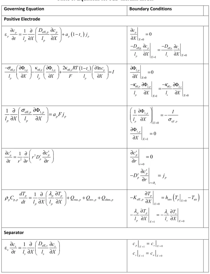
n L i J dx. (12)

Representative values for the parameter set obtained from the literature are given in the Appendix. Model equations for the P2D model are listed in Table 1.

Since the growth of the SEI layer is a function of the applied current and overpotential, optimal charging profiles can be developed that minimize the SEI layer growth, while ensuring the same capacity in a given time. Minimizing the SEI layer growth reduces the lost capacity, which in turn increases the cycle life. Various control strategies ranging from indirect methods to simultaneous discretization can be used to obtain the optimal profiles for Li-ion battery models. We implemented model-based optimal control to minimize the capacity fade for Li-ion batteries. To obtain the control profiles, a modified version of Control Vector Parameterization (CVP) was implemented and verified with simultaneous optimization strategies which are straightforward to apply for path-constrained problems. The mathematical formulation for minimizing the capacity fade due to SEI layer growth is

app( ) SEI SEI

0 0 min * f n t L i t Q A J dx dt   = − _ _  

∫ ∫

(13) 2 app 0 ≤ i ( ) t ≤ 54 A/m (14) 2.8 V ≤ ( ) V t ≤ 4.2 V (15) stored ≥16 Ahr Q (16)

subject to the model equations in Table 1.

This optimal control formulation and calculation is the exactly same as one step of model predictive control (MPC), which is the most commonly implemented advanced process control method implemented in industry and has been explored for application to lithium-ion battery operations.20,22,30-32 In MPC, the optimal control problem is solved at multiple sampling instances, based on the most recent measurements (for batteries, the measurements are voltage and temperature). The main advantage of MPC is that the online calculations account for the effects of model uncertainties and disturbances on the computed optimal control profiles; the main disadvantage is the online computational cost. A drawback of MPC is that the online computations expend energy, which reduces the amount of energy from the battery available for the use. As such, the appropriateness of online optimal control calculations for a particular battery application depends on the quantity of energy incurred by online calculations compared to the energy and battery lifetime savings that would be incurred by the online calculations and the total energy used for intended purpose of the battery. For example, the extra cost of online optimal control calculations would not be justifiable for an implantable cardiac pacer application,

in which online calculations would cause the battery to drain too quickly. Motivated by such small battery applications, the optimal control profile in this study computed for Cycle 1 was repeated for later cycles, rather than recomputed. For large battery applications, the optimal control profiles can be updated online based on new parameter values during each cycle, or once after each cycle or after many cycles.

The implemented control profile was obtained after trying to implement different profiles experimentally for a given cycle. We performed simultaneous discretization, conventional CVP, and a modified version of CVP to finally arrive at the optimal profile. Each of these approaches for calculating the optimal profiles is described below for the reformulated P2D model.

1) Simultaneous Discretization: In this approach, the governing partial differential equations are discretized in the spatial direction to generate ordinary differential equations (ODEs) in time. The ODEs are further discretized in time using Euler backward discretization to create a system of nonlinear algebraic equations. Although only first-order accurate, Euler backward was chosen due to its unconditional numerical stability and ease of demonstration. In this approach, both the control and state variables are discretized in temporal space. During optimization, this set of nonlinear equations acts as constraints. The objective function to be minimized was then defined as QSEI(tf), with the maximum charging current as 54 A/m2, and the

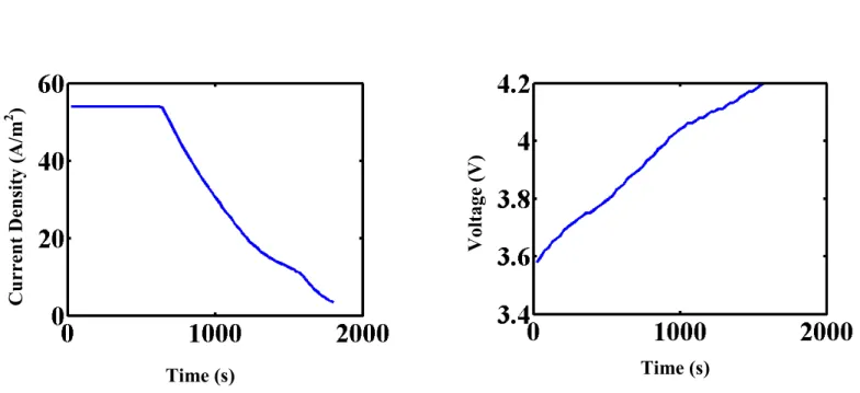
bounds on the voltage to be between 2.8 V and 4.2 V. The constraint on the total charge stored to be greater than 16 Ah was also implemented as defined in eq. (13)-(16) above. Note that the bounds on the manipulated variable (applied current in this case) and voltage of the cell were implemented by providing a bound on the resulting discretized variables for current and voltage at each discretized time point. The resulting nonlinear optimization was solved in IPOPT,33 which is based on an interior-point algorithm implemented in the C programming language, with the optimized current and voltage profiles shown in Figures 1a and 1b.

2) Control Vector Parameterization (CVP): In this approach, the total time horizon is divided into a finite number of time intervals. The manipulated variable (applied current) is assumed to be constant in each time interval, and the resulting optimization is solved for the discrete manipulated variables in each time interval. To explain further for this optimization, the total 1800 s time interval was divided into six time intervals, and the current was assumed to be

constant in the first four regions, until 1200 s. For example, the currents at the times 0, 300, 600, 900, 1200 s are given by i1, i2, i3, i4, i5, respectively. The current as a function of time is given by

1 2 app 3 4 5 4.2V , for 0 300 , for 300 600 ( ) , for 600 900 , for 900 1200 , for 1200 ₌ ≤ ≤   < ≤  = < ≤  _{< ≤}  < ≤  V i t i t i t i t i t i t T (17)

For the latter time period, the battery is charged with a constant current i5 until the voltage

reaches 4.2 V, after which the battery is charged at a constant voltage of 4.2 V for a total time of 30 minutes. For the control implementation, the optimization was solved for maximizing the charge stored in 1800 s, with a penalty on the capacity fade of the battery, that is,

app( ) app 0 max ( ) f f t t i t Q = A∗

∫

i t dt (18) 2 0 ≤ i_app( ) t ≤ 54 A/m (19) 2.8 V ≤ ( ) V t ≤ 4.2 V (20) SEI ≤0.5 SEI,max Q Q (21)

subject to model equations in Table 1, where

f

t

Q is the total capacity of the battery or the amount of charge stored in the battery, t is 30 minutes, and _f Q_SEI,maxis the maximum capacity lost to the SEI layer side reaction in a single cycle, which also means the capacity fade of the battery in a single cycle. This value was obtained from the experimental data after repeatedly cycling the battery at C/2 charge/1C discharge (Case A) as explained more in the next section.

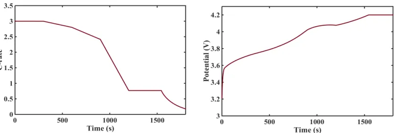
The resulting optimization is solved using NLPSolve optimizer in Maple 14, to find the optimal values of i1, i2, i3, i4, i5 in the specified time intervals, with the current and voltage

profiles shown in Figures 2a and 2b.

3) Modified CVP: This approach is a slight variation of the above CVP. The total 1800 s time interval was divided again into six time intervals, but in this case, the current was assumed to be varying linearly in the first four regions, until 1200 s. For example, the currents at the times 0, 300, 600, 900, 1200 s are given by i1, i2, i3, i4, i5, respectively. The current in each of the time

(

)

(

)

(

)

2 1 1 3 2 2 app 4 3 3 5 4 4 5 4.2V , for 0 300 300 0 300 , for 300 600 600 300 ( ) 600 , for 600 900 900 600 900 , for 900 1200 1200 900 , for 1200 ₌   −  +_{ } ≤ ≤  −     _{ − } + − ≤ ≤    −    =  −  +_{ } − ≤ ≤  _{ − }  −    +_{ } − ≤ ≤  −     ≤ ≤  V i i i t t i i i t t i t i i i t t i i i t t i t T (22)

After time t = 1200 s, the current i5 is assumed to be constant until the voltage reaches 4.2

V. Charging is at constant voltage after that until the total time is 1800 s. The optimization formulation is the same as in equations 18 to 21. The optimal control problem is solved in each of the regions using the NLPSolve optimizer in Maple 14, to obtain the optimal values for i1, i2,

i3, i4, and i5, with the optimal current and voltage profiles shown in Figures 3a and 3b.

From Figures 1ab, it can be seen that finally towards the end of charge in the simultaneous approach, the charging profile mimics the constant potential mode. In the implementation of the CVP and modified CVP approaches, assuming constant potential at the end decreased the optimization time and the number of stages, and provided a better objective function value. The total number of stages was chosen as 6, because increasing the number of stages any further did not have significant impact on the optimal value for the cell capacity. Since the current is continuous, there is no jump in potential as in the previous case.

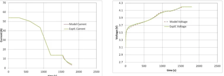
The current and voltage profiles obtained from experiments have good agreement with the model predictions for the simultaneous discretization, CVP, and modified CVP approaches (see Figures 4 to 6). The best agreement was for the modified CVP approach. The implementation of the conventional CVP and the modified CVP approach requires robust solvers to integrate highly stiff nonlinear equations in time. In the modified CVP approach, the assumption of a linear current profile in each time interval results in a continuous profile that avoids initialization issues for DAEs,34 whereas the conventional CVP approach leads to discontinuities and hence have DAEs that are harder to solve. As such, the modified CVP approach has lower computational cost and preferred for experimental implementation.

Experimental Validation

To quantify the benefits obtained from these control profiles, 16Ahr NMC pouch cells were cycled with the obtained charging profiles. In Case A, the cells were cycled under mild currents to obtain a baseline for the best-case performance of the cells. The cells were charged at a C/2 rate to 4.2 V, followed by a CV charge at 4.2 V until the charge current tapered off to C/10 (1.6 A) or less and then discharged at 1C rate to 2.8 V. In another set of cycling experiments, the cells were charged at the 2C rate until the cutoff voltage of 4.2 V was reached followed by a CV charge such that the total charge time was 30 minutes, followed by a 5C discharge to 2.8 V. This set of experiments is referred to as Case B. A third set of cells were charged with the optimal control profile for the same duration as Case B (i.e., 30 minutes) and discharged under identical conditions (i.e., 5C currents to 2.8 V), which is referred to as Case C. All the cycling experiments were performed in a controlled environmental chamber at 30oC. The optimization was formulated using

(1) Life estimates based on the cycling conditions from Case A. This case provides the values for Q_SEI,maxas mentioned above.

(2) Charge and life behavior from Case B.

(3) The Case C objective, minimize fade while charging in 30 minutes (with SEI layer growth at all the points less than 50% of Case B, making sure full charge was stored). This number needs to be as low as possible. If only 10% is indicated, please note that battery might not charge at all. The idea of this approach is to store the same charge while keeping the fade minimal. While strictly speaking, this is a pareto-optimal problem, only the best possible fade minimization with guaranteed charge stored was used.

Results and Discussion

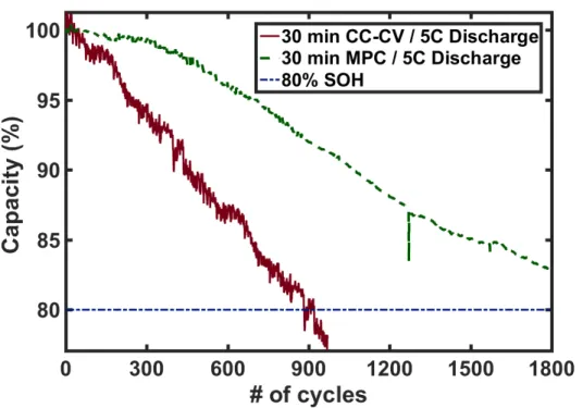
The profile in Figure 3a was used to charge the cells, which is referred to as “MPC” as discussed in the mathematical formulation. Figure 7 shows the experimentally determined reduction in capacity vs. number of cycles for the CC-CV case and the MPC case. While the battery charged with the CC-CV profile reaches end of life after around 900 cycles, the battery with the MPC profile cycles more than 1800 cycles before reaching end of life, which is a gain of more than 100% in cycle life.

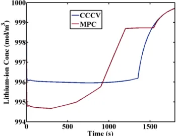
Figures 8 to 10 compare the concentration of lithium ions in the electrolyte solution at the cathode-current collector interface, cathode-separator interface, and the anode-separator interface respectively, for the CC-CV and the optimal control cases. As the battery charges, the concentration varies minimally with time in any of the regions. The shape of the concentration profiles mimics that of the current profile in the cathode as the concentration of lithium in the electrolyte decreases with time (compare Figs. 8 and 9 with Fig. 3a), whereas the reverse happens in the anode (compare Fig. 10 with Fig. 3a).

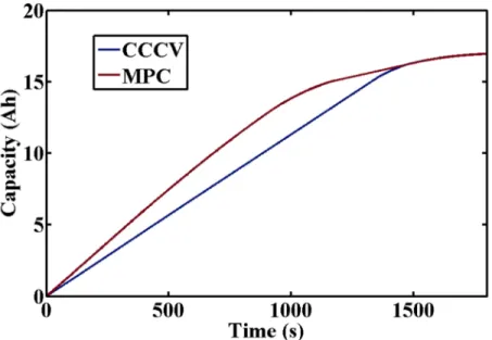
Figure 11 compares the battery capacity (charge stored) with time for the CC-CV and MPC cases. For the MPC case, more charge is stored at short times, compared to longer times when the battery undergoes higher fade. The CV charging phase is also shorter in the MPC case, compared to the CC-CV case. The final capacity in both cases is observed to be the same.

Figure 12 and 13 compare the overpotential vs. time, at the cathode-separator and the separator-anode interface, for the CC-CV and MPC cases. The overpotential at the cathode-separator interface are similar for both cases at most times, with the largest difference occurring between 1200 and 1400 s (Fig. 12). In contrast, the overpotential at the anode-separator interface are quite different for most of the time, with MPC being lower than the CC-CV case at short times and towards the end (Fig. 13). A lower overpotential leads to a decreased rate of the SEI-layer side reaction at the end, which reduces the capacity fade of the battery.

Figure 14 compares the capacity lost (QSEI) for the CC-CV and the MPC cases based on

the profile of the first cycle. While the total capacity of the battery after charging remains same (Fig. 11), the capacity lost during the charging is lower at the end of the charging for MPC than the CC-CV case (Fig. 14). With repeated cycling, the MPC profile continues to do a better job, resulting in a gain as is evident in Figure 7.

The optimal profile based on the first cycle using base parameters was impelmented until the battery reached its end of life. The end of life is defined as the number of cycles after which the battery reaches 80% of its initial capacity. This definition of end of life is consistent with many battery applications, including for most EV/PHEV batteries, so this definition was used to be consistent with an industry-prevalent standard practice. Without updating the control profile, we obtained in excess of 100% gain in cycle life of the cells as compared to the 2C CC-CV case

model with use would likely produce an even higher benefit. The relative improvement would be a function of the materials and chemistry of the battery, along with the temperature and the charging/discharging conditions in which the battery is used. Whether this benefit would be worth the extra energy costs of online optimal control calculations would depend on the specifics of the application, as discussed in the section on Optimal Model-based Control Formulations.

Conclusions

This article presents strategies for determining optimal charging profiles for lithium-ion batteries, to maximize their cycle life, while storing a given amount of charge in 30 minutes. Although not the main focus of this article, the modified-CVP approach implemented with the reformulated battery model is not computationally prohibitive, and could be used in real-time control. The optimal profile calculated for the first cycle of use was implemented on 16 Ah NMC cells at NREL. The optimal charging profiles were compared to the standard CC-CV charging method used for Li-ion batteries, with the CC charge rate of 2C. A gain of more than 100% in cycle life was observed using the predicted optimal charging profile.

Future work involves the development of an advanced self-learning battery management system (BMS), which would implement the standard MPC charging on a Li-ion battery of unknown chemistry. In this BMS, the parameters will be calculated and updated on the fly, in real time, based on the error in the voltage-time measurement. The optimal charging profiles will be calculated and updated every few cycles to maximize the capacity or cycle life based on the application the battery is being used in. The gain in life or capacity will be quantified after experimental validation at NREL. In our opinion, such a BMS has a potential to be a game-changer in the industry, and could help in faster adoption of Li-ion battery technology.

Acknowledgements

The authors acknowledge financial support from the U.S. Department of Energy (DOE), through the Advanced Research Projects Agency (ARPA-E) award number DE-AR0000275, and the Clean Energy Institute (CEI) at the University of Washington (UW) and the Washington Research Foundation (WRF).

Table 1: Equations for P2D thermal model

Governing Equation Boundary Conditions

Positive Electrode

(

)

eff, 1 ε ∂ = ∂ + 1− ₊ ∂ ∂ ∂     ∂   p p p p p p p p c a t j t l X D c l X eff,p eff,s 0 0 1 0 = = = ∂ = ∂ − ∂ − ∂ = ∂ ∂ s p p p s X X X c X D c D c l X l X

(

)

1, 2 eff, κeff, , 2κeff, 1 ln σ ₊ − ∂Φ ∂Φ − ∂ − + = ∂ ∂ ∂                   p p p p p p p p p RT t c I l X l X F l X 2, eff, 2, eff, 2, 0 0 1 0 κ κ = = = ∂Φ = ∂ − ∂Φ − ∂Φ = ∂ ∂ p p s s p p s X X X X l X l X eff, 1, 1 ∂ σ ∂Φ  =   ∂ _ ∂ _ p p p p p p a F j l X l X 1, , 1, 0 1 1 0 σ = = ∂Φ = − ∂ ∂Φ = ∂         p eff p p p X X I l X X 2 2 1 ∂ ∂ = ∂ ∂  _∂    ∂   s p s p s p c r D t r r c r 0 0 s s p r s p s p p r R c r c D j r = = ∂ = ∂ ∂ − = ∂ p, rxn, rev, ohm, 1 λ ρ = ∂  ∂ + + + ∂ _ ∂ _ p p p p p p p p p p dT T C Q Q Q

dt l X l X eff , env

(

0 air

)

0 = = ∂ − = − ∂ p p _{p X} X T K h T T X 0 1 p p s s X X p s T T l X l X λ λ = = ∂ ∂ − = − ∂ ∂ Separator eff, 1 ε ∂ = ∂  ∂  ∂ ∂ _ ∂ _ s s s s s s D c c t l X l X 0 1 1 0 = = = = = = s X X s X n X p c c c c

(

)

eff, 2, eff, κ ∂Φ 2κ 1− + ∂ln − + = ∂ ∂             s s s s s s RT t c I l X F l X 2 , 2 , ₀ 1 2 , ₁ 2 , ₀ = = = = Φ = Φ Φ = Φ p _{X s X} s _X n _X p, ohm, 1 λ ρ = ∂ _ ∂ _+ ∂ _ ∂ _ s s s s s s s s dT T C Q dt l X l X 1 0 0 1 | | | | X X X p s s n X T T T T = = = = = = Negative Electrode

(

)

eff, 1 ε ∂ = ∂ _ ∂ _+ 1− ₊ ∂ _n ∂ _ ∂ _ n n n n n n n l D c c a t j t X l X 1 1 0 eff, eff, 0 = = = = − = ∂ ∂ − ∂ ∂ ∂ ∂ s X X n X s n n s n l l c X D c D c X X

(

)

1, 2

eff, κeff, , 2κeff, 1 ln

σ ₊ − ∂Φ ∂Φ − ∂ − + = ∂ ∂ ∂                   n n n n n n n n nRT t c I l X l X F l X 2, ₁ 1 0 eff, 2, eff, 2, 0 κ κ = = = Φ = − = − ∂Φ ∂Φ ∂ ∂ s n X X n X s s n n l X l X

(

)

eff, 1, sei 1 _∂ σ ∂Φ  = +   ∂ _ ∂ _ n n n n n n a F j j l X l X 0 1, eff, 1, 1 0 1 σ = = = ∂Φ = − ∂ ∂Φ ∂ X n n n n X I l X X 2 2 1 ∂ ∂ = ∂ ∂  _∂    ∂   s s n n s n c r D t r r c r 0 0 s s n r s s n n n r R c r c D j r = = ∂ = ∂ ∂ − = ∂ p, rxn, rev, ohm, 1 λ ρ = ∂ _ ∂ _+ + + ∂ _ ∂ _ n n n n n n n n n n dT T C Q Q Q dt l X l X _{1 0} s s n n X X s n T T l X l X λ λ = = ∂ ∂ − = − ∂ ∂

(

)

eff, env air 1

1 = = ∂ − = − ∂ n n n X X T K h T T X

Table 2: Additional equations

(

)

rxn,i i i 1,i 2,i i , , Q =Fa j Φ − Φ −U i= p n rev,i i , , i i i U Q Fa j T i p n T ∂ = = ∂

(

)

2 2

1, 2, eff, 0 2,

ohm, eff, eff, 2

2 1 1 1 1 1 , , i i i i i i i i i i i i i RT c Q t i p n l X l X F l c X X κ σ  ∂Φ  κ  ∂Φ  ₊ ∂ ∂Φ =   +   + − = ∂ ∂ ∂ ∂    

(

)

2 2, eff, 0 2, ohm,s eff, 2 2 1 1 1 1 s s s s i s s s s RT c Q t l x F c l X X κ κ  ∂Φ  ₊ ∂ ∂Φ =   + − ∂ ∂ ∂  

(

)

(

) (

)

ref

,ref ref ref

,θ = ,θ + − _ _ , = ,   i i i i i i i T dU U T U T T T i p n dT r f ,eff e 1 1 exp  , , = _− _ − __ =     s i D a s s i i E D D i p n R T T ,eff ref 1 1 exp  , , = _−  − _ =     i a i i k E k k i p n R T T

Table 3: List of parameters

Symbol Parameter Positive

Electrode Separator Negative Electrode Units i σ Solid-phase conductivity 100 100 S/m , f i ε _{Filler fraction} 0.025 0.0326 i ε _Porosity 0.385 0.724 0.485

Brugg _{Bruggman coefficient} 4

D _{Electrolyte diffusivity} 10 7.5 10× − 10 7.5 10× − 10 7.5 10× − m2/s s i D _{Solid-phase diffusivity} 14 1.0 10× − 14 3.9 10× − m2/s i

k _{Reaction rate constant} 11

2.334 10× − 11 5.031 10× − mol/(s m2)/(mol/m3)1+αa,i ,max s i c Maximum solid-phase concentration 51554 30555 mol/m3 ,0 s i c Initial solid-phase concentration 25751 26128 mol/m3 0 c Initial electrolyte concentration 1000 mol/m3

,

p i

R _{Particle radius} 2.0×10-6 2.0×10-6 M

ai Particle surface area to

volume

885000 723600 m2/m3

i

l _{Region thickness} 80×10-6 25×10-6 88×10-6 M

t_{+ Transference number} 0.364

F _{Faraday’s constant} 96487 C/mol

R _{Gas constant} 8.314 J/(mol K)

ref T _Temperature 298.15 K ρ _Density 2500 1100 2500 kg/m3 CP _{Specific heat} 700 700 700 J/(kg K) Λ _{Thermal conductivity} 2.1 0.16 1.7 J/(m K) s i a D E

Activation energy for temperature-dependent solid-phase diffusion 5000 5000 J/mol i a k E

Activation energy for

temperature-dependent reaction constant

Figures

Figure 1: (a) Current vs. time and (b) voltage vs. time profiles computed for the simultaneous discretization approach.

Figure 2: (a) Current vs. time and (b) voltage vs. time profiles computed for the CVP approach. C u rr en t D en si ty ( A /m 2 ) C u rr en t D en si ty ( A /m 2 ) V ol tage ( V ) Time (s) Time (s) V ol tage ( V )

Figure 3: (a) Current vs. time and (b) voltage vs. time profiles computed for the modified CVP approach.

Figure 4: Comparison of experimental and predicted (a) current vs. time and (b) voltage vs. time profiles obtained using simultaneous discretization.

Figure 5: Comparison of experimental and predicted (a) current vs. time and (b) voltage vs. time profiles for CVP approach.

Figure 6: Comparison of experimental and predicted (a) current vs. time and (b) voltage vs. time profiles for the modified CVP approach.

Figure 7: Capacity vs. number of cycles for 2C CC-CV and the MPC profiles, where “MPC” refers to the optimal charging profile obtained by the modified CVP approach.

Figure 9: Lithium-ion concentration at the cathode-separator interface.

Figure 11: Capacity of the battery vs. time for the CC-CV and MPC profiles.

Figure 12: Overpotential at the cathode-separator interface for the CC-CV and MPC profiles.

Figure 13: Overpotential at the anode-separator interface for the CC-CV and MPC profiles.

Figure 14: Capacity fade of the battery vs time for the first cycle for the CC-CV and MPC profiles.

References

1.

http://energy.gov/technologytransitions/articles/battery500-consortium-spark-ev-innovations-pacific-northwest-national, Battery500 Consortium to Spark EV Innovations: Pacific Northwest National

Laboratory-led, 5-year $50M Effory SEEKS to Almost Triple Energy Stored in Electric Car Batteries, in Department of Energy, US Website (2016).

2. E. Wesoff, How Soon Can Tesla Get Battery Cell Costs Below $100 per Kilowatt-Hour?, in

http://www.greentechmedia.com/articles/read/How-Soon-Can-Tesla-Get-Battery-Cell-Cost-Below-100-per-Kilowatt-Hour (2016).

3. A. Bizeray, S.R. Duncan and D.A. Howey, Advanced battery management systems using fast electrochemical modelling, in Proceedings of IET Hybrid and Electric Vehicles Conference 2013 (HEVC

2013), London, UK (2013).

4. G. L. Plett, Battery management systems, Volume I: Battery modeling, Artech House Publishers (2015). 5. V. Ramadesigan, V. Boovaragavan, J.C. Pirkle Jr., and V.R. Subramanian, Journal of the

Electrochemical Society, 157, A854 (2010).

6. V. R. Subramanian, V. Ramadesigan, and M. Arabandi, Journal of the Electrochemical Society, 156, A260 (2009).

7. V. R. Subramanian, V.D. Diwakar, and D. Tapriyal, Journal of the Electrochemical Society, 152, A2002 (2005).

8. P. W. C. Northrop, V. Ramadesigan, S. De, and V.R. Subramanian, Journal of the Electrochemical

Society, 158, A1461 (2011).

9. P. W. C. Northrop, M. Pathak, D. Rife, S. De, S. Santhanagopalan, and V.R. Subramanian, Journal of

the Electrochemical Society, 162, A940 (2016).

10. M. Doyle, T.F. Fuller, and J. Newman, Journal of the Electrochemical Society, 140, 1526 (1993). 11. G. Ning, R.E. White and B.N. Popov, Electrochimica Acta, 51, 2012 (2006).

12. V. Ramadesigan, P.W.C. Northrop, S. De, S. Santhanagopalan, R.D. Braatz, and V.R. Subramanian,

Journal of the Electrochemical Society, 159, R31 (2012).

13. H. Rahimi-Eichi, and Mo-Yuen C., in Proceedings of the IECON 2012 - 38th Annual Conference on

IEEE Industrial Electronics Society, Montreal, Quebec, Canada (2012).

14. R. C. Kroeze, and P.T. Krein, in Proceedings of the Power Electronics Specialists Conference

(PESC),IEEE (2008).

15. D. Zhang, B.N. Popov and R.E. White, Journal of the Electrochemical Society, 147, 831 (2000). 16. S. Santhanagopalan, Q. Guo, P. Ramadass and R.E. White, Journal of Power Sources, 156, 620 (2006).

17. R. N. Methekar, V. Ramadesigan, R.D. Braatz, and V.R. Subramanian, ECS Transctions, 25, 139 (2010).

18. S. K. Rahimian, S.C. Rayman and R.E. White, Journal of the Electrochemical Society, 157, A1302 (2010).

19. B. Suthar, P.W.C. Northrop, R.D. Braatz,and V.R. Subramanian Journal of the Electrochemical

Society, 161, F3144 (2014).

20. J. Liu, G. Li and H.K. Fathy, Journal of Dynamic Systems, Measurement and Control, 138, 021009 (2016).

21. H. E. Perez, X. Hu and S.J. Moura, Proceedings of the American Control Conference (ACC), 4000 (2016).

22. R. Klein, N.A. Chaturvedi, J. Christensen, J. Ahmed, R. Findeisen, and A. Kojic, in Proceedings of

the American Control Conference (ACC), San Francisco, CA, USA, 382 (2011).

23. A. Hoke, A. Brissette, K. Smith, A. Pratt, and D. Maksimovic, IEEE Journal of Emerging and

Selected Topics in Power Electronics, 2, 691 (2014).

24. V. Ramadesigan, K. Chen, N.A. Burns, V. Boovaragavan, R.D. Braatz, and V.R. Subramanian,

25. K. B. Hatzell, A. Sharma, and H.K. Fathy, in Proceedings of the American Control Conference

(ACC), Montreal, Canada, 584 (2012).

26. J. C. Forman, S.J. Moura, J.L. Stein, and H.K. Fathy, Journal of Power Sources, 210, 263 (2012). 27. S. Santhanagopalan, Q. Guo, and R.E. White, Journal of the Electrochemical Society, 154, A198 (2007).

28. D. D. Speltino C., G. Fiengo, and A. Stefanopoulou, in Proceedings of the European Control

Conference, Budapest (2009).

29. P. Ramadass, B. Haran, P. M. Gomadam, R. White and B. N. Popov, Journal of the Electrochemical

Society, 151, A196 (2004).

30. M. Torchio, L. Magni, R.D. Braatz, and D.M. Raimondo, in Proceedings of the 11th IFAC Symposium

on Dynamics and Control of Process Systems, including Biosystems, Trondheim, Norway, 827 (2016).

31. M. Torchio, N.A. Wolff, D.M. Raimondo, L. Magni, U. Krewer, R.B. Gopaluni, J.A. Paulson, and R.D. Braatz, in Proceedings of the American Control Conference (ACC), Chicago, IL, USA, 4536 (2015). 32. B. Suthar, V. Ramadesigan, P.W.C. Northrop, B. Gopaluni, S. Santhanagopalan, R.D. Braatz, and V.R. Subramanian, in Proceedings of the American Control Conference (ACC), Seattle, WA, USA, 5350 (2013).

33. A. Wachter, and L.T. Biegler, Mathematical Programming, 106, 25 (2006).

34. M. T. Lawder, V. Ramadesigan, B. Suthar, and V.R. Subramanian, Computers and Chemical