Experimental and numerical study of turbulence in fusion plasmas using reflectometry synthetic diagnostics

HAL Id: tel-01868530

https://tel.archives-ouvertes.fr/tel-01868530v2

HAL is a multi-disciplinary open access

archive for the deposit and dissemination of sci-entific research documents, whether they are pub-lished or not. The documents may come from teaching and research institutions in France or abroad, or from public or private research centers.

L’archive ouverte pluridisciplinaire HAL, est destinée au dépôt et à la diffusion de documents scientifiques de niveau recherche, publiés ou non, émanant des établissements d’enseignement et de recherche français ou étrangers, des laboratoires publics ou privés.

Experimental and numerical study of turbulence in

fusion plasmas using reflectometry synthetic diagnostics

Georgiy Zadvitskiy

To cite this version:

Georgiy Zadvitskiy. Experimental and numerical study of turbulence in fusion plasmas using reflec-tometry synthetic diagnostics. Plasma Physics [physics.plasm-ph]. Université de Lorraine; Universität Stuttgart (Allemagne), 2018. English. �NNT : 2018LORR0074�. �tel-01868530v2�

AVERTISSEMENT

Ce document est le fruit d'un long travail approuvé par le jury de

soutenance et mis à disposition de l'ensemble de la

communauté universitaire élargie.

Il est soumis à la propriété intellectuelle de l'auteur. Ceci

implique une obligation de citation et de référencement lors de

l’utilisation de ce document.

D'autre part, toute contrefaçon, plagiat, reproduction illicite

encourt une poursuite pénale.

Contact : ddoc-theses-contact@univ-lorraine.fr

LIENS

Code de la Propriété Intellectuelle. articles L 122. 4

Code de la Propriété Intellectuelle. articles L 335.2- L 335.10

http://www.cfcopies.com/V2/leg/leg_droi.php

´

Ecole doctorale EMMA Institut f¨ur Grenzfl¨achenverfahrenstechnik

Colledge Sciences et Technologies und Plasmatechnologie

Th´ese

pour l’obtention du grade de

Docteur de l’Universit´

e de Lorraine pr´

esent´

ee par:

Georgiy Zadvitskiy

Pr´epar´ee au sein de l’Institut Jean Lamour, IGVP, University of Stuttgart et IRFM, CEA, Cadarache

Experimental and numerical study of

turbulence in fusion plasmas using

reflectometry synthetic diagnostics

Stephane Heuraux Professeur, IJL, Universit´e de Lorraine Directeur de th´ese Sebastien Hacquin CEA, IRFM, F-13108 Saint-Paul-lez-Durance Co-directeur de th´ese G¨unter Tovar Professor, IGVP, Universit¨at Stuttgart Co-directeur de th´ese

Pascale Hennequin Directrice de Recherche CNRS, DR2 Raporteur

Evgeniy Gusakov Professor, Ioffe Physico-Technical Institute Raporteur

Ulrich Stroth Professor, Technical University Munich Examinateur

J¨org Starflinger Professor, IKE, Universit¨at Stuttgart Examinateur Michel Vergnat Professeur, IJL, Universit´e de Lorraine Examinateur

IJL - Universit´

e de Lorraine, IGVP - University of Stuttgart,

IRFM - CEA, Cadarache

Declaration

I declare that this thesis was composed by myself and that the work contained therein is my own, except where explicitly stated otherwise in the text.

To my daughter Olivia, who was born during second year of

my Ph.D. studies

Acknowledgements

These 3 and half years which I spent on my Ph.D. dissertation were very interesting and productive. I have learned a lot and grown in many ways. I want to thank people who helped me during this time and were supporting me along the way. First I want to thank Prof. Stephane Heuraux who directed and organized my work, solved all administrative issues which were complected by double degree between University of Lorraine and University of Stuttgart, and by co-financement from Cadarache. He showed me the world of reflectometry helped me with numerical tools has improved my knowledge during many hours of discussions.

I want to thank Prof. G¨unter Tovar for guiding and accelerating administrative process in University of Stuttgart. Also I want to thank Prof. Thomas Hirth for supervising me during first part of my work.

I am thankful to Dr. Carsten Lecte letting me to use his code, helping with com-putations and for technical support, Dr Sebastien Hacquin for his scientific advices and intensive editing of my poor English texts. Dr. Roland Sabot with who I had many discussions being in Cadarache and Dr. W. Kasparek who was leading meet-ings in Stuttgart University. I wish to thank Dr. Frederic Clairet for giving me his reflectometry interpretation results for JET tokamak.

This work would be not completed without my visit to IPP Garching. I am thankful to Dr. Garrard D. Conway who agreed my visit and gave me the possibility to work with ASDEX-U data, Dr. Anna Medvedeva who helped me with data extraction and shared her results for comparisons. I want to thank Dr. Dmitrii Prisiazhniuk for number of very useful discussions that has answered many of my questions.

Particularly I want to thanks Prof. E. Z. Gusakov for very important discussion related to theoretical models and data analysis. Also I want to thank Dr. Mikhail Irzak for useful mail exchange which allowed me to use reciprocity theorem.

Very big computations performed in this work would be impossible without help of bwUniCluster in Baden-W¨urttemberg.

I wish to acknowledge the support and help of my friends: Mr. Dr. Jordan Cavalier, Artur Vander Sande, Dr. Antom Bogomolov, Dr. Rennan Marales. Jordan Ledig,

Homam Betar, Julien M´edina, Oleg Krutkin, Liza Sytova, Richard Deutsch, Anton Kyyanytsa, Dr. Georgiy Kichin, Krishnan Srinivasarengan and others. If I forgot somebody it doesn’t mean I don’t appreciate your help, it is just my “good” memory.

I want to thanks members of the music bands where I was playing. These people helped me to mix my scientific work with some art and make it more interesting and productive. Dr. Yusuf Bhujwalla, Masha Usoltceva, Valentin Pascu, Aaron Ho, Marcella Tizo, Michal Kuczynski, Wojciech Trl and a cover band from Cadarache.

I want to thank my wife Vitalina for giving me the Daughter and supporting me all the time. My daughter Olivia which was my ray of light in the final part of the Ph.D. In the end I want to thank my parents which always were always supporting my interest in physics and mathematics. Thanks you, you made me to be who I am.

Аннотация

Ыстық плазмадағы энергия мен бөлшектерге ауытқыма ауысуы турбуленттiлiкпен тығыз байланысты. Сондықтан болашақ термоядролық электростанциялардың тиiмдiлiгiн арттыруда турбуленттiлiктi зерттеу өте маңызды. Бұл жұмыс тығыздық профилiн және плазма турбуленттiлiгiнiң толқындық радиалды спектрiн өлшеуге арналған, бүкiл әлемде таралған ТОКАМАКтарда кеңiнен қолданылатын шамадан тыс рефлектометрия мәлiметтерiн талдауға арналған. Турбуленттiлiктiң төмен деңгейiнде рефлетометр дыбысын талдау өте қарапайым, ол тығыздықтың жоғары деңгейдегi наразылығы жағдайында қиындай түседi. Мысалы, бұл жұмыста зондтау толқынының бұғатталуы әсерiнен пайда болатын резонанстар рефлектометр фазасының ауытқуын тудыруға қабiлеттi екенi көрсетiлген. Әдетте турбуленттiлiктiң ең жоғары деңгейi плазмалық бағанның шекарасында байқалады. Турбуленттiлiк қабатымен қиылысында фазаның өзгеруi және сынақ сәулесiнiң кеңейуi плазмалық бағанның орталық аймақтарындағы спектрдi өлшеуге әсер етуi мүмкiн. Оның әсерi ұзын

корреляциялық ұзындығы жағдайында күшейедi. Алайда, қысқа корреляция ұзындығы керi Брегг шашырауына алып келедi және ол да дыбысты өзгертуге қабiлеттi. Турбуленттiлiктiң толқындық сандарын зерттеуде рефлектометр дыбысының фазасымен қатар дыбыстың амплитудасы да қолданылуы мүмкiн. Дыбыс фазасымен салыстырғанда амплитуда резонанстық секiрулерге ұшырамайды, сонымен қатар, дыбыс амплитудасын зерттеу арқылы турбуленттiлiктi әлдеқайда сапалы сипаттау мүмкiн болады. Турбуленттiк амплитудасы плазмалық шекарада максималға жеткен жағдайда оны жергiлiктi Брегг резонансы аймағында спектралды шыңның көмегiмен тiркеуге болады. Полоидальды тартылған антеннамен жабдықталған шамадан тыс рефлектометрия көмегiмен антеннаның орын ауыстыруымен бiрге спектральды шыңның орын ауыстыруын бақылауға болады. Шыңның орын ауыстыруы турбуленттi қабаттың күйi мен қасиеттерi туралы қосымша ақпарат алуға мүмкiндiк бередi.

Tore-Supra Токамагында GYSELA гиро-кинетикалық кодының ақпараттарын талдаушы көпжиiлiктi рефлектометрия жағдайында синтетикалық дигностиканы

үлгiлеуде екiөлшемдi толық толқынды код қолданылды. Дыбыс амплитудасы

көмегiмен өлшенген радиалды корреляциялық ұзындық турбуленттiлiктiң корреляциялық ұзындығына сәйкес келедi. Толық толқынды код, сонымен қатар, ASDEX-Upgrade

Токамагында шамадан тыс рефлектометрия жағдайында толқындық спектрдi және корреляциялық ұзындықты талдауда қолданылды. Бiрөлшемдi кодпен салыстыру әр түрлi нәтижелер көрсеттi. Алайда, екiөлшемдi және бiрөлшемдi кодтар негiзiндегi

синтетикалық диагностика көмегiмен есептелген корреляциялық ұзындық турбуленттiлiктiң корреляциялық ұзындығымен бiрдей реттi мәндердi қабылдайды.

Abstract

Anomalous energy and particle transport is closely related to micro-turbulence. There-fore plasma turbulence studies are essential for successful operation of magnetic confine-ment fusion devices. This thesis deals with the developconfine-ment of interpretative models for Ultra-Fast Swept Reflectometry (USFR), a diagnostic used for the measurement of turbulence radial wave-number spectra in fusion devices. While the interpretation of reflectometry data is quite straightforward for small levels of turbulence, it becomes much trickier for larger levels as the reflectometer answer is no longer linear with the turbulence level. It has been shown for instance that resonances due to probing field trapping can appear in turbulent plasma and produce jumps of the signal phase. In the plasma edge region the turbulence level is usually high and can lead to a non-linear regime of the reflectometer response. The loss of probing beam coherency and beam widening when the probing beam crosses the edge turbulence layer can affect USFR core measurements. Edge turbulence with a long correlation length leads to small beam widening and strong distortion of the probing wave phase. However backscattering ef-fects from turbulence with short correlation lengths are also able to cause reflectometer signal change.

To study turbulence wave-number spectra as well as reflectometer signal phase variations, signal amplitude variations can be analized. Unlike signal phase variation, amplitude does not suffer from resonant jumps, and can give more clear qualitative evaluation of turbulence structure. In the case when the turbulence amplitude peaked in the edge region, it can be detected as spectral peak near local Bragg resonance wave-number. USFR with a set of receiving antennas arranged poloidally was proposed to obtain more information on the edge turbulence properties. A displacement of the spectral peak appears when the receiving antenna is misaligned with the emitting one. Peak displacement measurements could provide additional information on probing beam shaping and turbulence properties and help in coherent mode observation as well. A 2D full wave code was applied as a synthetic diagnostic to Gysela gyro-kinetic code data to study Tore-Supra tokamak core turbulence. Radial correlation lengths computed from the amplitude of multi-channel fixed frequency reflectometry signals

have shown good agreement with the turbulence correlation length directly computed from the simulation. The synthetic diagnostic was then applied to analyse the cor-relation length and wave-number spectra obtained by USFR in the ASDEX-Upgrade tokamak. A comparison between 1D and 2D results have shown different behaviour. However correlation lengths measured with UFSR signals are in the same order with turbulence ones.

Contents

List of used variables 14

1 Introduction 21

1.1 Sources of the energy . . . 22

1.2 Nuclear fusion . . . 24

1.2.1 Introduction to nuclear fusion . . . 24

1.2.2 Ignition criterion . . . 25

1.2.3 Magnetic confinement fusion . . . 27

1.2.4 Tokamak magnetic configuration . . . 28

1.2.5 Parameters of the tokamaks used in this work . . . 30

1.3 Plasma turbulence . . . 31

1.3.1 Heat and particle transport in tokamak plasmas . . . 31

1.3.2 Tokamak turbulence wave-number spectrum . . . 33

1.3.3 Drift wave turbulence . . . 34

1.3.4 Core plasma instabilities . . . 35

1.3.5 Geodesic acoustic mode (GAM) . . . 36

1.3.6 Scope of the work . . . 37

2 Ultra fast sweeping reflectometry 39 2.1 Waves in magnetized plasmas . . . 39

2.1.1 Plasma dielectric tensor . . . 39

2.1.2 Ordinary mode (O-mode) . . . 41

2.1.3 Extraordinary mode (X-mode) . . . 41

2.1.4 Electromagnetic wave cut-off and resonances . . . 42

2.1.5 Wave propagation trough inhomogeneous plasmas . . . 43

2.1.6 Approximation of Wentzel-Kramer-Brillouin . . . 44

2.1.7 Wave propagation through a turbulent medium . . . 45

2.1.8 Mathieu equation . . . 45

2.2.1 Reflectometery basic principle . . . 47

2.2.2 Homodyne IQ detection . . . 49

2.2.3 Heterodyne IQ detection . . . 49

2.2.4 Other reflectometry types . . . 50

2.3 Closed loop algorithm . . . 51

3 Reflectometer response computation methods 53 3.1 Helmholtz equation . . . 53

3.2 Solution of 1D Helmholtz equation . . . 54

3.2.1 4th Order Numerov’s method for Helmholtz equation . . . 54

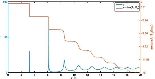
3.2.2 Electric field amplification phenomena . . . 55

3.2.3 Numerical precision of the Numerov’s method in the case of strong electric field amplification . . . 58

3.2.4 Numerical precision of the Numerov’s method with noisy density profile . . . 61

3.3 Time dependent wave-equation numerical solution . . . 64

3.3.1 1D Wave equation solver IQ detection technique . . . 65

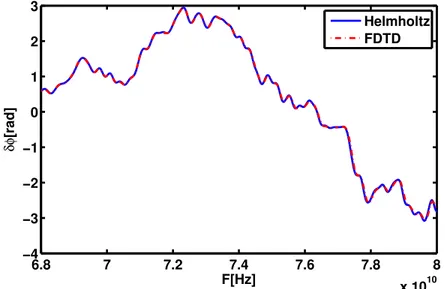
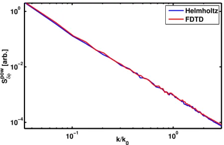
3.4 Comparison between 1D Helmholtz equation solver and time dependant 1D wave equation solver . . . 66

3.4.1 2D FDTD algorithm . . . 72

3.5 Reciprocity theorem approach . . . 75

3.5.1 Reciprocity theorem in application to reflectometry modeling . . 77

3.5.2 Reduced reciprocity theorem approach . . . 78

3.5.3 Reduced reciprocity theorem application example . . . 79

3.6 Discussions . . . 82

4 Strong edge turbulence effects on reflectometer plasma core measure-ments 83 4.1 Probing beam propagation through turbulent plasma . . . 83

4.1.1 Beam properties change in turbulent plasma. Modeling examples 84 4.2 Study of edge turbulence effects on reflectometer signal . . . 92

4.2.1 Edge turbulence effects on reflectometer phase spectra using edge-core k-spectra separation . . . 92

4.2.2 Edge turbulence effects on reflectometer signal in slab geometry 95 4.2.3 Mono wave-number mode observation through strong turbulence level . . . 99

4.2.4 Edge turbulence effects on reflectometer signal for Tore-Supra 2D profile . . . 102

4.3 Discussions . . . 106

5 Application to gyro-kinetic simulations data and experimental mea-surements 107 5.1 Synthetic diagnostic application to GYSELA gyro-kinetic simulation . . 107

5.2 ASDEX-Upgrade UFSR synthetic diagnostic . . . 111

5.2.1 Phase fluctuation and amplitude fluctuation spectra . . . 113

5.2.2 Turbulence correlation length measurements . . . 117

5.2.3 Conclusions and discussion . . . 120

Summary 121

R´esum´e 125

Bibliography 130

A Isotropic turbulence generation 139

B Miller equilibrium for shaped turbulence 145

List of used characters

Character Description units

𝐴 amplitude of reflectometer signal [𝑉 ]

𝐴0 amplitude of reflectometer emitted signal [𝑉 ]

𝑎𝑓 refraction index perturbation envelop [-]

𝐴𝑖 Helmholtz equation differential scheme coefficient in chapter 3 [-]

𝐴𝑖 RMS turbulence amplitude envelop in Appendix B [-]

𝑎𝑖 Mathieu equation stable solution function [-]

𝐴𝑟 amplitude of reflectometer received signal [𝑉 ]

𝐴𝑟𝑒𝑓 amplitude of reference signal [𝑉 ]

𝐴𝜔 reciprocity theorem complex coefficient [-]

𝑎 turbulence RMS amplitude fit coefficient [-]

𝐵 magnetic field strength [𝑇 ]

𝑏 turbulence RMS value fit coefficient [-]

𝑏𝑖 Mathieu equation stable solution function [-]

𝐵𝑖 Helmholtz equation differential scheme coefficient in chapter 3 [-]

𝛽 trapped particle banana orbit width [𝑚]

𝑐 speed of light [𝑚/𝑠]

𝐶𝑖 Helmholtz equation differential scheme coefficient in chapter 3 [-]

𝐷𝑛 density gradient transport coefficient [𝑚2/𝑠]

𝐷𝑇 temperature gradient transport coefficient [1/𝑚/𝑠/𝐾]

𝑑𝑓 refractive index perturbation envelop width [𝑚]

𝐷𝜔 electric displacement field of frequency 𝜔 [𝑉 /𝑚]

𝛿𝐸 electric field perturbation [𝑉 /𝑚]

𝛿𝐵 magnetic field strength perturbation [𝑇 ]

𝛿𝑇 temperature perturbation [𝐾]

𝛿𝑛 density perturbation [𝑚3]

𝛿𝜑 phase variation [𝑟𝑎𝑑]

𝑒 electron index [-]

𝐸𝛼 alpha particle energy [𝐽 ]

𝐸𝐺 GAM electric field [𝑉 ]

𝐸𝜔 electric field harmonic with circular frequency 𝜔 [𝑉 /𝑚]

𝐸𝑜𝑢𝑡 electric filed of reflected wave [𝑉 /𝑚]

𝐸𝑤𝑔 electric filed fundamental mode of the wave-guide [𝑉 /𝑚]

𝜖0 vacuum dielectric permittivity [𝐹/𝑚]

𝐹 frequency [Hz]

𝑓0 frequency sweep start frequency [Hz]

𝑓𝑟 neutron yield [1/𝑚3/𝑐]

𝐹𝑚 low frequency reflectometer oscillator frequency [𝐻𝑧]

𝐹𝑏 beat frequency [𝐻𝑧]

Γ𝑗 particle flux of specie "j" [1/𝑚2/𝑠]

Γ𝛿

𝑗 particle flux of specie "j" associated with turbulence [1/𝑚2/𝑠]

𝐻𝜔 magnetic field strength harmonic with circular frequency 𝜔 [𝑉 /𝑚]

ℎ numerical scheme resolution [-]

𝐻𝑤𝑔 magnetic filed of the fundamental mode of the wave-guide [𝑇 ]

ℎ𝑒 X-mode correction coefficient [-]

𝑖 imaginary unit [-]

𝐼𝑠 _{sin part of complex reference reflectometer signal [𝑉 ]}

𝐼𝑐 _{cos part of complex reference reflectometer signal [𝑉 ]}

𝐼 complex reflectometer signal [𝑉 ]

𝐼_𝑟𝑒𝑓𝑠 sin part of complex received reflectometer signal [𝑉 ]

𝐼𝑐

𝑟𝑒𝑓 cos part of complex received reflectometer signal [𝑉 ]

𝐼𝑖𝑛 unperturbed reflectometer signal [𝑉 ]

𝐼𝑠 turbulence related reflectometer signal [𝑉 ]

𝐽 current density [𝐶/𝑠/𝑚2_]

𝑘 electromagnetic wave wave-number [𝑚2_]

𝑘0 electromagnetic wave vacuum wave-number (except section 1.2.2) [𝑚2]

𝑘𝑏 Boltzmann constant (only in section 1.2.2) [𝑚2]

𝑘𝑠𝑐𝑎𝑡 scattered field wave-number [𝑟𝑎𝑑/𝑚]

𝑘𝑡𝑢𝑟𝑏 turbulence wave-number [𝑟𝑎𝑑/𝑚]

𝑘𝑖𝑛𝑐 incident beam wave-number [𝑟𝑎𝑑/𝑚]

𝑘𝑓 refractive index perturbation wave-number [𝑟𝑎𝑑/𝑚]

𝜅 coherent field attenuation coefficient [-]

𝑙𝑛𝑐 density fluctuation correlation length across the magnetic field [𝑚]

Λ Numerov’s method operator [-]

𝜆 wave-length [𝑚]

𝑚𝛼 particle mass of specie "𝛼" [𝑘𝑔]

𝜇0 The magnetic constant [𝑁/𝐴2]

𝑁 refractive index [-]

𝑛 electron plasma density (except section 3.3) [1/𝑚3]

𝑛 time-step index (only in section 3.3) [1/𝑚3_]

𝑛𝑖 plasma density of specie "i" [1/𝑚3]

𝑛𝐺 GAM density fluctuation [𝑚3]

𝑛𝐺

0 GAM density fluctuation amplitude [𝑚3]

𝑛𝑐 electromagnetic wave critical electron density [𝑚−3]

𝑁0 refractive index of unperturbed plasmas [-]

𝑃𝐻𝑒𝑥 external heating power [𝑊 ]

𝑃𝐻𝛼 power received from fusion alpha-particles [𝑊 ]

𝑃𝑛𝑒𝑢𝑡𝑟𝑜𝑛 power produced by fusion neutrons [𝑊 ]

𝑃𝑙𝑜𝑠𝑠𝑒𝑠 power losses from the plasma [𝑊 ]

𝑝 Mathieu equation parameter [-]

𝜑 phase (except chapter 1) [𝑟𝑎𝑑]

Φ electric potential [𝑉 ]

Φ𝐺 _{GAM electric potential [𝑉 ]}

𝜑 poloidal angle (only in chapte 1) [𝑟𝑎𝑑]

𝜑𝑟 phase of reference signal [𝑟𝑎𝑑]

𝜑𝑟𝑒𝑓 phase of reflected signal [𝑟𝑎𝑑]

𝜑𝑣𝑎𝑐𝑢𝑢𝑚 phase of reflected wave obtained in the vacuum region [𝑟𝑎𝑑]

𝜑0 initial beam phase [𝑟𝑎𝑑]

𝜋 pi constant [-]

𝑄 fusion reactor efficiency coefficient [-]

𝑞 charge (except 2.1.8) [𝐶]

𝑞 Mathieu equation parameter (only in section 2.1.8) [-]

𝑞𝛼 charge of specie "𝛼" [𝐶]

𝑟𝑖 radial position of computational grid-point "𝑖" [𝑚]

𝑅 radial position [𝑚]

𝜌 Larmor radius [𝑚]

𝑆_𝛿𝑛𝑝𝑜𝑤 density perturbation wave-number power spectrum [𝑚−6]

𝑆_𝛿𝜑𝑝𝑜𝑤

0 experimental phase variation power wave-number spectrum [𝑟𝑎𝑑

2_𝑚]

𝑆𝑤𝑔 wave-guide surface [𝑚2]

𝑆𝐴 modulus of signal amplitude variation wave-number spectrum [𝑉 ]

𝑆𝑐 modulus of complex reflectometer signal wave-number spectrum [𝑉 ]

𝑆𝛿𝜑 modulus of reflectometer signal phase variation wave-number spectrum [𝑟𝑎𝑑] ∧

𝜎 plasma conductivity tensor [𝐶/𝑠/𝑚/𝑉 ]

𝜎 fusion reaction cross-section [𝑚2_]

𝑇 𝑟 transfer function [𝑟𝑎𝑑2_𝑚]

𝑇𝑖 temperature of specie "i" [𝐾]

𝑇 temperature [𝐾]

𝑡 time [𝑠]

𝜏𝑛𝑐 density fluctuation correlation time [𝑚]

𝜏𝐸 energy confinement time [𝑠]

𝜃 toroidal angle [𝑟𝑎𝑑]

𝑉 plasma volume [𝑚3]

𝑣 particle velocity [𝑚/𝑠]

⃗𝑣𝐵×𝐹 𝐵 × 𝐹 drift velocity in presence of external force [𝑚/𝑠]

⃗𝑣𝐵×𝑔𝑟𝑎𝑑𝐵 𝐵 × 𝑔𝑟𝑎𝑑𝐵 drift velocity in presence of magnetic field gradient [𝑚/𝑠]

⃗𝑣𝐸×𝐵 𝐸 × 𝐵 drift velocity in presence of electric field [𝑚/𝑠]

𝑣𝑐 sound velocity [𝑚/𝑠]

𝑣𝐺 _{GAM particles velocity [𝑚/𝑠]}

𝑣𝑓 frequency sweeping rate [Hz/s]

𝑊 weighting function [𝑉2_]

𝜔 circular frequency [𝑟𝑎𝑑/𝑠]

𝜔𝑐 electron cyclotron frequency [𝑟𝑎𝑑/𝑠]

𝜔𝑝 plasma osculation circular frequency [𝑟𝑎𝑑/𝑠]

𝜔𝑈 𝐻 upper hybrid resonance circular frequency [𝑟𝑎𝑑/𝑠]

𝜔𝐻 X-mode high cut-off circular frequency [𝑟𝑎𝑑/𝑠]

𝜔𝐿 X-mode low cut-off circular frequency [𝑟𝑎𝑑/𝑠]

𝜔𝑠𝑐𝑎𝑡 scattered field circular frequency [𝑟𝑎𝑑/𝑠]

𝜔𝑖𝑛𝑐 incident beam circular frequency [𝑟𝑎𝑑/𝑠]

𝜔𝑡𝑢𝑟𝑏 turbulence circular frequency [𝑟𝑎𝑑/𝑠]

𝑥 coordinate [𝑚]

𝑥𝑓 refraction index perturbation envelop position [𝑚]

𝜉1 turbulence RMS value fit coefficient [-]

𝜉2 turbulence RMS value fit coefficient [-]

𝑦 poloidal coordinate [𝑚]

Chapter 1

Introduction

Figure 1.1: Primary energy consumption by different regions in the last 50 years with time extrapolation. Sourced from [1]

Nowadays growing world demands for energy and ecological restrictions applied on classic energy sources make us look for new renewable sources of energy. Renewable energy sources are sources which could be renewed on the human time-scale or Inex-haustible during much longer time then human time-scale. For the last 30 years world energy consumption has grown by more than 2.5 times (figure 1.1). As we see on figure 1.1 in Europe and North America this consumption level growth has decreased in last years. This is due to growing cost of the energy, more efficient energy use due to developed technologies, advanced ecological norms and redistribution of factories in direction of Asian-Pacific regions. Conversely in Asia-Pacific regions including so called developing countries, due to the growth of population and fast industrial

de-velopments, energy consumption grows very fast. But as it happened in developed European countries, after some time this growth should slow down. However even at current consumption rate, the ecological situation requires new green energy sources.

1.1

Sources of the energy

It is possible to separate available energy sources in 3 groups [2]. ∙ Chemical energy: coal, oil, gas, fossil fuels;

∙ Nuclear energy: fission of uranium or thorium, fusion of light elements(deuterium, tritium);

∙ Renewable energy: hydro, wind, solar, thermal, photo voltaic, geothermal [3], [4], [5]

Figure 1.2: Primary energy consumption by fuel with extrapolation in time. Sourced from [1]

Electricity production from chemical energy usually connects with large 𝐶𝑂2 emis-sion and air pollution with substances such as nitrogen oxides [6] which are very harmful for life nature. Figure 1.2 shows that in the past and at this moment the main part of the energy production comes from the first category, chemical energy. This has produced a big impact on the "global warming problem" [7]. Considering renewable energy sources (RES), wind and sun energy at the moment covers only 3% of the total

Figure 1.3: An example of produced solar power during one year in Germany. Figure taken from [8]

produced energy (see figure 1.2). These energy sources are not constant in time and re-quire good backup and/or energy storage. Hydro power is less than 7% and the growth of this source is quite limited by irregular geographical location. Modern fission based on breeder reactor technology with fast neutrons could be a good candidate to replace old fission reactors and burning of fossil fuels. This technology can sufficiently reduce nuclear waste and increase safety. Unlike conventional reactors which uses uranium-234 it can use other isotopes of uranium and other heavy nucleus. This solves problem of limited amount of Uranium-234. Unfortunately distrust of fission in general from the civil society is too strong for these reactors to become widely used in recent future.

With limited use of nuclear power plants and burning of fossil, fuels countries should rely more on RES. Power generated by these sources vary much in time. An example of solar generated power variation is presented on figure 1.3. To provide power level able to support peaks of the power consumption, a wide network of different types of RES should be created [2]. This network should include backup systems in case there will be temporal decrease of RES output power, for instance backup gas power plant can be used. At the moment there is no technology to store big amounts of energy. It was shown that the entire RES network in Europe and the United States is not efficient unless some technological breakthroughs will happen [2, 9].

1.2

Nuclear fusion

Another solution which can become available in the end of the century is magnetic confinement nuclear fusion. In this section we will have a look on plasma tokamak confinement basics and highlight concepts needed for this thesis work presentation. However more precise information could be found in the following sources [10, 11].

1.2.1

Introduction to nuclear fusion

The idea behind nuclear fusion comes from the sun. Sun energy is produced by fusion of light atoms. But unlike the sun, earth fusion will use more effective is sense of energy yield deuterium-tritium (D-T) reaction and in perspective D-D reaction. In order to fuse atoms should first overcome an electric repulsion. This is possible only at very high energy (10 − 20𝑘𝑒𝑉 ). Ionized gas where particles have that energy should be confined to maintain the required high density. High densities are needed to have high fusion rate (1.1):

𝑓𝑟 = 𝑛1𝑛2 < 𝜎𝑣 > (1.1)

where 𝑛1 and 𝑛2 are the density of fusion species, 𝜎 is the fusion reaction cross-section, and 𝑣 is the relative velocity of fusing atoms. This expression gives information on how many reactions are produced per second in the volume unit. Because of a relatively larger cross-section for smaller energies, deuterium-tritium (D-T) plasma reaction was chosen to make earth fusion. Table 1.1 shows possible reactions and reaction product energy from D-T plasmas. Figure 1.4 represents cross-sections of these reactions. As

fusing species products and its energies

𝐷 + 𝑇 𝐻𝑒4₂(3.56𝑀 𝑒𝑉 ) + 𝑛𝑒𝑢𝑡𝑟𝑜𝑛(14.03𝑀 𝑒𝑉 )

𝐷 + 𝐷 𝐻𝑒3

2(0.82𝑀 𝑒𝑉 ) + 𝑛𝑒𝑢𝑡𝑟𝑜𝑛(2.45𝑀 𝑒𝑉 )

𝐷 + 𝐷 𝑇 (1.01𝑀 𝑒𝑉 ) + 𝐻(3.02𝑀 𝑒𝑉 )

𝐷 + 𝐻𝑒3₂ 𝐻𝑒4₂(3.71𝑀 𝑒𝑉 ) + 𝐻(14.64𝑀 𝑒𝑉 )

Table 1.1: Fusion reactions and products

one can see from this figure, 𝐷 − 𝑇 reaction has the highest rate with a maximum reached for temperatures near 100𝑘𝑒𝑉 . A 14.03𝑀 𝑒𝑉 neutron is a product of this reac-tion. This fast neutron’s energy is then to be transferred to electricity. Alpha particles resulting from the same reaction will be used to transfer its energy to the main plasma species. Hydrogen is the most distributed nuclei in universe. Its isotope deuterium is stable and distributed quite well on the Earth. In the ocean, for 6420 atoms of hydro-gen there is one atom of deuterium. Tritium will be produced using lithium and fast

Figure 1.4: Cross-sections of possible nuclear reactions. Averaging is done using Maxwellian velocity distribution function. Figure source: "Encyclopedia of Energy", Volume 4. (Elsevier Inc., 2004)

neutrons from main fusion reaction (Table1.2). Fusion can be considered as renewable

fusing species products

𝑛𝑒𝑢𝑡𝑟𝑜𝑛 + 𝐿𝑖6 𝑇 + 𝐻𝑒4₂ 𝑛𝑒𝑢𝑡𝑟𝑜𝑛 + 𝐿𝑖7 _{𝑇 + 𝐻𝑒}4

2+ 𝑛𝑒𝑢𝑡𝑟𝑜𝑛

Table 1.2: Tritium production reactions

energy source as amount of deuterium and tritium is enough to power humanity for millions of years [12]. Cross-sections of the two 𝐷 − 𝐷 reactions are very close to each other, which gives a probability of 50% each. However these cross-sections are much smaller than the cross-section of 𝐷 − 𝑇 and 𝐷 − 𝐻𝑒3

2 reactions.

1.2.2

Ignition criterion

As shown in figure 1.4, fusion requires very high temperatures. But to be used as energy source fusion reactors should fulfil a few other conditions. Hot plasmas have quite strong convection and diffusion of heat and particles, which means that in any case energy losses take place. They can be described by energy confinement time 𝜏𝐸, which is the characteristic time of energy loss by the plasma without external heating. Fusion plasmas can be heated by fast fusion alpha particles and external heating. Now we can express the energy balance when the total plasma heating is equal to the plasma losses.

Where 𝑃𝐻𝑒𝑥 is an external heating power, 𝑃𝐻𝛼 is the plasma heating power received from alpha particles. Let’s look on what plasma parameters are crucial for fusion device. 𝑃𝐻𝛼= 1 4𝑛 2 _{< 𝜎𝑣 > 𝐸} 𝛼𝑉 (1.3)

Expression (1.3) is calculated for the most optimal case when the plasma consists only of deuterium and tritium in equal proportions. 𝐸𝛼 = 3.56𝑀 𝑒𝑉 is in the fusion 𝛼 particle born energy, 𝑉 is the plasma volume, and 𝑛 is the plasma density.

𝑃𝑙𝑜𝑠𝑠𝑒𝑠≈ 3𝑛𝑘𝑏𝑇 𝑉 /𝜏𝐸 (1.4)

3𝑛𝑘𝑏𝑇 𝑉 is an estimating formulation of the plasma kinetic energy content, where 𝑇 is the temperature and 𝑘𝑏 - the Boltzmann constant. From formulas (1.2-1.4) one can express the needed external heating power to maintain burning plasma conditions:

𝑃𝐻𝑒𝑥 = ( 3𝑛𝑘𝑏𝑇 𝜏𝐸 − 1 4𝑛 2 _{< 𝜎𝑣 > 𝐸} 𝛼)𝑉 (1.5)

Without external heating we will achieve the so-called ignition criterion when losses are fully compensated by fusion 𝛼 particles power.

𝑛𝜏𝐸 >

12𝑘𝑏𝑇 < 𝜎𝑣 > 𝐸𝛼

(1.6) < 𝜎𝑣 > of the 𝐷 − 𝑇 reaction can be approximated with 10% accuracy in the range of 6-20 keV to:

< 𝜎𝑣 >≈ 1.1 · 10−24𝑇2 (1.7)

This allows us to calculate the so-called triple product criterion.

𝑛𝜏𝐸𝑇 > 3 · 1021[𝑚−3𝑘𝑒𝑉 𝑠] (1.8)

This simple estimation can give us an idea on the main parameters values which should be achieved for successful fusion reactor prototype construction. At the moment there are 2 main concepts: inertial fusion, and magnetic confinement fusion (MCF). In in-ertial fusion solid state fuel target is compressed and heated by multiple laser rays homogeneously distributed over its surface. With this method plasma density is very high while energy confinement time is short. On the contrary magnetic confinement fusion relies on energy confinement time of few seconds and small densities. Typical target values that MCF tries to achieve are: 𝑛 = 1020_𝑚−3_{, 𝑇 = 10𝑘𝑒𝑉 , and 𝜏}

𝐸 = 3𝑠

Figure 1.5: Charged particle drift in magnetic field with external force. Plasma ions and electrons are drifting in opposite directions. Picture has been taken from [13]

efficiency coefficient 𝑄 can be estimated as:

𝑄 = 𝑃𝑛𝑒𝑢𝑡𝑟𝑜𝑛/𝑃𝐻𝑒𝑥 (1.9)

Here we don’t take into account the energy transfer efficiency from energetic neutrons to electricity. This will be done by transfer heat from the blanket wall which will be irradiated by fusion neutrons. Also it is important to mention that most neutron yield is coming from the high energy tail of ion velocity distribution function. Heating methods like neutral beam injection, ion cyclotron resonance heating (ICRH) or lower hybrid resonance heating and current drive (LHCD) enlarge the high energy tail of the velocity distribution function. These fast ions are expected to generate significant part of fusion neutrons.

1.2.3

Magnetic confinement fusion

The sun confines its fusion plasma using strong gravitation forces. On the Earth this mechanism is not applicable. As plasmas consist of charged particles they can be caged by magnetic field. With the magnetic field charged particles are moving as spirals, around magnetic lines with the Larmor radius 𝑟𝑙 = 𝑚𝑣_𝑞𝐵⊥. Here 𝑣⊥ is the particle velocity projection on perpendicular direction to magnetic field. If an external force applied to the particles it creates a constant velocity motion called drift (1.10).

⃗𝑣𝐵×𝐹 = 1 𝑞

[ ⃗𝐹 × ⃗𝐵]

𝐵2 (1.10)

Here ⃗𝐹 and ⃗𝐵 are vectors of external force and magnetic field respectively. Figure 1.5 shows particle trajectories during drift motion. In MCF this force can be created by

gravitation, electric field, magnetic field gradient, temperature or pressure gradients and magnetic lines curvature. There are two main machine design concepts that are designed to limit this motion in a predefined volume. They are tokamaks and stellara-tors. Both are based on the similar idea to close magnetic lines in a circle. This will create a toroidal magnetic configuration in which particles are moving along magnetic lines. But such a configuration results in magnetic field that decreases with the major radius. This magnetic field gradient creates a drift of plasma ions and electrons (1.11).

vB×gradB = 𝐾⊥

𝑞𝐵

[ ⃗𝐵 × 𝑔𝑟𝑎𝑑𝐵]

𝐵2 (1.11)

Where 𝐾⊥ is perpendicular kinetic energy. This drift is directed in opposite directions for ions and electrons. It creates charge separation and vertical electric field. Vertical electric field will also create a drift (1.12) which will move the whole plasma outside the torus and limit energy confinement time by this movement.

vE×B =

[ ⃗𝐸 × ⃗𝐵]

𝐵2 (1.12)

Simple toroidal magnetic configuration results in plasma self movement, the same way as did famous Baron M¨unchhausen.

Not far from the other side I fell into the bog. Here I would have undoubt-edly died, if not the strength of my own arm, grabbing my own pigtail, had pulled me, including my horse—which I squeezed tightly between my legs-out of it (Baron M¨unchhausen)

The way how this problem is solved is the main difference between tokamaks and stellarators. More details will be given in next section.

1.2.4

Tokamak magnetic configuration

To avoid vertical electric field effect one can twist the magnetic lines around small cross-section of the torus (in poloidal direction). As ions and electrons move freely along the magnetic lines, in other words plasma conductivity along the magnetic lines is very high (see section 2.1.1), this poloidal magnetic lines transformation will con-nect upper and down sides of the machine with magnetic lines. Current along these magnetic lines will remove the electric field produced by vertical charge separation. The current which cancel this electric field is called Pfirsch-Schl¨uter current. The main difference between tokamaks and stellarators is that stellarators produce such a mag-netic field poloidal rotation using complex shape of magmag-netic coils whereas tokamaks

Figure 1.6: a) tokamak basic coil design and plasma shape b) stellarator coils with curved plasma, picture inspired by www.ideen2020.de/wpcontent/uploads/slideshow-gallery/5_tokamak_stellarator_a_RGB.jpg (entered 17.06.2018)

have a toroidal plasma current which creates a poloidal twist of the magnetic field lines (figure 1.6). In this work we will focus on the tokamak geometry. Readers can find more information about stellarators in [14]. In the tokamak configuration toroidal coils which create the toroidal magnetic field are combined with the central solenoid column. The column itself is a transformer core and the plasma loop is a secondary coil. This solenoid is made to drive the plasma toroidal current. Due to horizontal forces which try to expand the plasma loop, additional coils are required for the equilibrium. These forces are:

1)Pressure: Along the magnetic lines over one magnetic surface, the pressure stays constant. However the inner surface of the torus is smaller than the outer surface. This results in pressure force that is stronger on outer side than on inner one.

2)Toroidal current: the current loop always has an expanding force created by interac-tion with its own magnetic field.

To compensate these forces in the tokamak, vertical magnetic field coils are used. These coils create a vertical magnetic field which interacts with the plasma current, then cre-ating a horizontal force directed towards the plasma current loop center. In modern tokamaks plasmas usually are shaped to be elliptically elongated and triangular. In divertor tokamaks [15] the last closed magnetic surface has a so-called X-point. This X-point directs plasma flow from the separatrix to a specially designed plate (divertor). This technology helps to decrease the power loads on the first wall. Additional shaping coils are used to obtain the desirable magnetic eqilibrium. On figure 1.7 is represented the magnetic coil configuration of the ASDEX-upgrade tokamak.

Figure 1.7: ASDEX-upgrade tokamak poloidal cross-section with magnetic coils con-figuration. Picture inspired by www.ipp.mpg.de/4324839/original-1517424707.jpg (en-tered 17.06.2018)

1.2.5

Parameters of the tokamaks used in this work

In my thesis work part of the reflectometry computations were done using real tokamak geometry and density profiles. These tokamaks are: Tore-Supra, JET (Joint European Torus), and ASDEX-Upgrade (Axially Symmetric Divertor EXperiment). In this sec-tion main parameters of these machines are introduced.

Parameter max(typical) JET ASDEX-Upgrade Tore-Supra

Location Culham, UK Garching, Germany CEA Cadarache, France

Cross-section D-shaped D-shaped Circular

minor radius [m] 1.25-2.1 0.5-0.8 0.7 major radius [m] 3 1.65 2.4 plasma volume [m3_{] 100 13 25} B [T] 3.45 (2.5-3.2) 3.1 (2.5) 4.2 (3.75) I [MA] 4.8 (2.5) 1.6 (0.4-1.4) 1.4 (0.5-1.2) 𝑛𝑒 [𝑚−3] 2 · 1019-1.1 · 1020 < 1019 1 · 1019-9 · 1020 pulse duration [s] <30 <10 <400

No experimental work was performed by the author. All data used in the simula-tions were used under collaboration with various groups: Tore-Supra (S. Hacquin, F. Clairet, G. Dif-pradalier, R. Sabot), ASDEX-Upgrade (F. Clairet, A. Medvedeva), and JET (F. Clairet).

1.3

Plasma turbulence

1.3.1

Heat and particle transport in tokamak plasmas

In tokamak plasmas density and temperature are not homogeneous. Due to the toka-mak geometry and radial transport, particle density and temperature are peaked in the plasma core. Plasma density profile can vary with minor radius up to a few or-ders of magnitude. In section 1.2.2 we saw that for advanced performances of a fusion power plant, energy confinement time 𝜏𝐸 is a very critical parameter. This parame-ter is mostly defined by plasma instabilities and plasma turbulence as they drive heat and particle transport in a tokamak. Turbulence is usually present in tokamak dis-charges. Numerous experiments have shown fluctuations of many plasma parameters as plasma density 𝛿𝑛, temperature 𝛿𝑇 , plasma potential 𝛿𝜑, plasma current density 𝛿𝐽 , electric and magnetic fields 𝛿𝐸, 𝛿𝐵. Further information can be found in N. Bretz’s pa-per [16].To express the connection between turbulence and anomalous transport let us look at the generalized form of the transport coefficients. Anomalous fluxes of bilinear correlations of perturbations can be written according to Ross [17]

Γ𝑗 = −𝐷𝑛 𝜕𝑛𝑗 𝜕𝑟 − 𝐷𝑇 𝜕𝑇𝑗 𝜕𝑟 + 𝑣𝑛𝑗+ Γ 𝜕 𝑗 (1.13) 𝑄𝑗 = −𝜒𝑗𝑇𝑛𝑗 𝜕𝑇𝑗 𝜕𝑟 − 𝜒𝑗𝑛𝑇𝑗 𝜕𝑛𝑗 𝜕𝑟 + 𝑣𝑛𝑗𝑇𝑗 + 5 2𝑘𝑏𝑇𝑗Γ𝑗 + 𝑄 𝛿 𝐽 (1.14)

Where Γ𝑗 and 𝑄𝑗 are ambipolar particle and energy fluxes of species 𝑗. The total flux consists of a sum of terms defined by Coulomb collisions (neoclassical transport) and Γ𝛿 fluxes associated with turbulence (anomalous transport), 𝐷 and 𝜒 are respec-tively transport coefficients of particle and temperature, 𝑣 is the convectional velocity. Anomalous particle and energy fluxes driven by 𝐸 × 𝐵 drift can be associated with variations of electric field 𝛿𝐸 as one expects the magnetic particle diffusion term to be negligible.

Γ𝛿𝐸_𝑗 = ⟨𝛿𝑛𝑗𝛿𝑣𝑟⟩ = ⟨𝛿𝐸𝜃𝛿𝑛𝑗⟩/𝐵𝜑 (1.15) Here 𝜃 is the poloidal angle, 𝜑 is the toroidal angle, 𝑟 means radial coordinate, and ‖ and ⊥ signs are related to the magnetic field direction. Drift turbulence energy flux

can be expressed the same way. 𝑄𝛿𝐸_𝑗 = −3 2𝑘𝑏𝑛𝑗⟨𝛿𝐸𝜃𝛿𝑇𝑗⟩/𝐵𝜑+ 3 2𝑘𝑏𝑇𝑗⟨𝛿𝐸𝜃𝛿𝑛𝑗⟩/𝐵𝜑 (1.16) Convectional flux 𝑄𝛿𝐸_{𝑐𝑜𝑛𝑣} = 5₂𝑘𝑏𝑇𝑒

𝐵𝜑 ⟨𝛿𝐸𝜃𝛿𝑛𝑒⟩ can be calculated if both 𝛿𝑛𝑒 and 𝛿𝐸𝜑 are measured simultaneously. However by means of wave scattering, reflectometry, electron cyclotron emission, and beam emission spectroscopy only 𝛿𝑛 of 𝛿𝑇 can be measured and additional assumptions should be added to compute energy and particle fluxes.

Assuming a specific type of turbulence, one can simplify the task. Electrostatic drift waves are driven by plasma pressure gradient and could appear in many regions of tokamak plasmas. For all electrostatic modes a general expression can be written.

𝛿𝑛𝑒 𝑛𝑒

𝑠𝑖𝑛(𝜓) = 𝑒𝛿Φ 𝑘𝑏𝑇𝑒

; 𝑘𝜑𝛿Φ = −𝛿𝐸𝜑 (1.17)

In this expression 𝜓 is the phase between 𝛿𝑛𝑒 and 𝛿Φ - the plasma potential. The particle flux in this case can be expressed as:

Γ𝛿𝐸_𝑗 = 𝑛𝑒𝜐𝑇 𝑒𝜌𝑐𝑒⟨ 𝛿𝑛2 𝑒 𝑛2 𝑒 𝑘𝜃sin(𝜓)⟩ (1.18) Here 𝜐𝑇 𝑒𝜌𝑐𝑒 = 𝑐_𝑒𝐵𝑇 𝑒

𝜑 and 𝜐𝑇 𝑒 =√︀𝑘𝑏𝑇𝑒/𝑚𝑒is the thermal speed, and 𝜌𝑐𝑒 = 𝜐𝑇 𝑒/𝜔𝑐𝑒is the electron cyclotron radius. There is a theory [18] as well as experimental observations [19] to express the phase 𝜓. However in this subsection, for simplicity we will consider limiting the expression under conditions of strong turbulence which is called mixing length limit, when 𝛿𝑛𝑒/𝑛𝑒 ≈ 1/𝑘𝑟𝐿𝑛 ≪ 1, sin(𝜓) ≈ 1 where 𝐿𝑛 is the density gradient length 1/𝐿𝑛 = −𝑑(ln(𝑛𝑒))/𝑑𝑟. Under isotropy assumption 𝑘𝑟 ≈ 𝑘𝜃 we can find:

𝐷_𝑛𝛿𝐸(𝑠𝑡𝑟𝑜𝑛𝑔𝑡𝑢𝑟𝑏𝑢𝑙𝑒𝑛𝑐𝑒) ≈ 𝜐𝑇 𝑒𝜌𝑐𝑒 𝛿𝑛𝑒

𝑛𝑒

(1.19) Such conditions are typical for plasma core where density fluctuation 𝛿𝑛𝑒/𝑛𝑒< 1%

Another way to estimate the particle diffusion coefficient is based on the general random walk using averaged space step across the magnetic field and correlation time.

𝐷𝛿𝐸_𝑛 (𝑟𝑎𝑛𝑑𝑜𝑚𝑤𝑎𝑙𝑘) ≈ 𝑙_𝑛𝑐2 /𝜏𝑛𝑐 (1.20)

where 𝑙𝑛𝑐 and 𝜏𝑛𝑐 are correlation length and time of density fluctuations across the magnetic field.

Using these expressions one can conclude that to experimentally investigate particle and energy transport nature one has to measure fluctuations of density 𝛿𝑛,

temper-Figure 1.8: (a) Turbulence energy spectrum by Kolmogorov’s theory. Direct cascades with 𝑘−5/3dependence; (b) Turbulence energy spectrum predicted by Kraichnan-Leith-Batchelor’s model, with direct cascade 𝑘−3 and inverse cascade 𝑘−5/3

ature 𝛿𝐸, plasma potential 𝛿Φ, electric and magnetic fields 𝛿𝐸 and 𝛿𝐵. This thesis work will be focused on density perturbations properties measurements with microwave reflectometry.

1.3.2

Tokamak turbulence wave-number spectrum

Aside from electrostatic drift wave turbulence which was considered in previous section 1.3.1 other electrostatic modes were found to be source of anomalous transport: MHD-like modes driven by magnetic field curvature, ripple losses, viscosity, plasma current, electromagnetic skin depth modes [20], and thermal instabilities in plasma edge [21]. MHD-like modes have significantly longer wavelength comparing to skin depth mode and drift wave modes are sitting in between them.

In a tokamak, the turbulence energy obtained from free energy of pressure gradient can be transferred between turbulent modes with different wavelengths and frequencies. Moreover this energy can be exchanged with zonal flows and geodesic acoustic modes (GAM). GAM will be discussed in section 1.3.5. Frequency and wave-number spectra contain very important information, which allow us to verify theoretical models used in numerical modelling.

Numerous theoretical works were done to describe the turbulence behaviour. Kol-mogorov’s well-known work [22] describes homogeneous isotropic turbulence in 3D fluid. This model gives turbulence energy cascades in the direction of small scale turbulence (so called direct cascade) with spectral behaviour 𝑘−5/3 figure 1.8(a). Energy propa-gates to smaller scale turbulence where viscosity plays a major role and leads to energy dissipation.

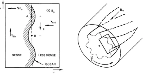
Figure 1.9: illustration of drift wave developing mechanism for adiabatic electrons. Reproduced from [11]

As tokamak plasmas are not isotropic due to the magnetic field 2D description is more natural. Under such conditions Kraichnan-Leith-Batchelor’s (KLB) model was developed [23]. This model predicts direct energy cascade with typical 𝑘−3 dependence towards high wave-number direction from energy injection region (scale where energy is received by turbulence from kinetic instabilities), and energy cascade in the direction of smaller wave-number (inversed cascade) with 𝑘−5/3 (figure 1.8(b)).

1.3.3

Drift wave turbulence

Drift wave instability is a basic linear instability. It could appear in plasmas with homogeneous magnetic field and density gradient. Periodic perturbation of electric field potential 𝛿Φ perpendicular to the direction of density gradient is assumed. Because of the electrons low mass they react fast on these perturbations. This results in charge separation in the direction perpendicular to the density gradient. The electric field appearing during this charge separation together with the magnetic field produces a particle drift. Under the approximation of adiabatic electrons (𝛿𝑛𝑒 = 𝑒𝛿Φ_𝑇𝑒 𝑛𝑒) the phase relation between potential variation phase and density perturbation doesn’t make this perturbation unstable but leads to vertical drift with diamagnetic velocity (see figure 1.9). But in the case of collisions (plasma resistivity) this phase difference changes and the density perturbation becomes unstable and particles from higher density regions moves to smaller density regions.

1.3.4

Core plasma instabilities

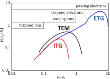
In the plasma core region the density gradient doesn’t reach high values as in the plasma edge region. However temperature profile is peaked closer to the plasma center. In this region ITG (ion temperature gradient), which is believed to be a major reason of anomalous ion temperature transport [24, 25], dominates ETG (electron temperature gradient) [26], trapped electron mode (TEM) [27], and trapped ion mode(TIM) [28,29, 30]. These turbulent modes have different typical scale lengths. The scale is connected to Larmor radius 𝜌 for passing particles and banana orbit width 𝛽 for trapped particles. In the case of typical tokamak setup:

𝛽𝑖 > 𝜌𝑖 ≥ 𝛽𝑒 > 𝜌𝑒 (1.21)

where indexes 𝑒 and 𝑖 mean electrons and ions.

Ion temperature gradient modes: small wave-number turbulence. Usually the most important modes in tokamak in terms of transport. It is driven by ion temperature gradient and can be stabilized by density gradient. They can also be stabilized by increase of impurities concentration. However impurities can have their own ITG instability with different frequencies due to their mass.

Trapped ion modes: the largest scale instabilities. Because of their scale they can induce strong transport. But these instabilities generally make small contribution to total transport. However when ITG are suppressed TIM should be taken into account for good turbulence representation [28].

Electron temperature gradient modes: Large wave-number instabilities. Be-cause of their small scale they don’t contribute much to transport. In the case of electron heating they can give large contribution to electron transport [31].

Trapped electron modes: Rising from temperature or density gradient, from interaction between electromagnetic waves and trapped electrons. They can be damped by collisionality as it vanishes velocity distribution function and decreases the number of trapped electrons. Also the magnetic shear can cause a stabilizing effect [32].

Figure 1.10: Instability growth rate 𝛾 as a function of normalized wave-number 𝑘𝜃𝜌𝑖. Where 𝑘𝜃 is poloidal wave-number. Picture inspired by [33]

1.3.5

Geodesic acoustic mode (GAM)

Geodesic acoustic modes were named after similar phenomena in the planet atmosphere and were first discovered by N. Winsor [35]. Local (zonal) flows oscillate proportionally to the sound velocity 𝑣𝑐 divided by the major radius. These flows are caused by radial potential variations. In the round cross-section toroidal tokamak shape these potential perturbations can be expressed as:

Φ𝐺(𝑟) = 𝐴𝐺(𝑟)𝑒𝑥𝑝(−𝑖𝜔𝑡) (1.22)

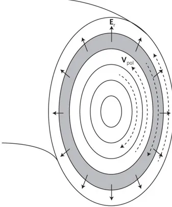
And the electric field which is associated with this potential can be found as 𝐸𝐺 ₌ −𝑑Φ𝐺_{/𝑑𝑟. This electric field leads to a poloidal plasma drift in addition to the main} rotation caused by not perturbed radial field (see figure 1.11).

𝑣𝐺= −𝑐𝐸𝐺/𝐵 (1.23)

Particle flows created by this velocity are called zonal flows. In inhomogeneous mag-netic field divergence of such fluxes does not equal to zero. It should be compensated by particle flows along magnetic field lines. These flows will change their direction with initial potential variations. Amplitude of these flows is proportional to cos(𝜃), where 𝜃 is the poloidal angle. Parallel velocity is equal to:

Figure 1.11: Toroidal tokamak cross-section with zonal GAM flows and radial electric field variation. Picture source - [36]

Parallel velocity also oscillates in time with cycle frequency 𝜔. These fluxes should be created by pressure gradient along the magnetic lines, created by periodic density modulation:

𝑛𝐺 = 𝑛𝐺₀ sin(𝜃) (1.25)

To summarize, radial electric potential fluctuations give birth to poloidal and toroidal zonal flows, which lead to electric field perturbation modes with poloidal wave number 𝑚 = 0, and density perturbation mode with 𝑚 = 1. GAMs correspond to coherent structure which we will try to detect using reflectometry in the next chapters.

1.3.6

Scope of the work

Good understanding of turbulent transport and its prediction possibilities are essen-tial for thermonuclear reactor design and operation. Diagnostic of plasma turbulence demands high temporal and spatial resolution. In the case of thermonuclear reactor there are limited number of diagnostics available. Plasma region situated close to the first wall can be investigated using Langmuir probes which is limited to operation in relatively cold plasmas [37]. Turbulence in the tokamak plasma core can be studied using technique called beam emission spectroscopy (BES) [38]. A very well-established technique that is expected to be the main turbulence diagnostic in ITER [39] is

reflec-tometry [40]. It is very flexible and can measure different turbulent modes as well as MHD instabilities, it has minimal excess requirements and can be used under strong neutron yield from plasma.

In this work applicability of the ultra-fast swept reflectometry (UFSR) will be in-vestigated using 2D full wave code. The plan of the report is as follows:

Chapter 2: Electromagnetic waves in plasma physics basics will be introduced. Prin-ciple of reflectometer work will be explained.

Chapter 3: Numerical methods for reflectometry synthetic diagnostic will be high-lighted.

Chapter 4: Reflectometer signal change by strong edge turbulence layer will be stud-ied.

Chapter 5: Synthetic diagnostic will be applied to gyro-kinetic code data in Tore-Supra tokamak and based on experimental data in ASDEX-Upgrade tokamak.

Chapter 2

Ultra fast sweeping reflectometry

In this chapter I will highlight the theory behind wave propagation in magnetized plasmas. Also reflectometer principles and basic signal analysis will be presented.

2.1

Waves in magnetized plasmas

Next we will highlight basic physics behind reflectometer electromagnetic wave propa-gation into magnetized tokamak plasmas.

2.1.1

Plasma dielectric tensor

Now let us look on plasma particles motion in high frequency electromagnetic waves. Plasmas consist of ions and free electrons. Motion equations for these species look like:

⎧ ⎪ ⎪ ⎪ ⎨ ⎪ ⎪ ⎪ ⎩ 𝑑𝑣(𝛼)𝑥/𝑑𝑡 = 𝑞𝛼𝐸𝑥/𝑚𝛼+ 𝑞𝛼𝑣(𝛼)𝑦𝐵𝑧/𝑚𝛼 𝑑𝑣(𝛼)𝑦/𝑑𝑡 = 𝑞𝛼𝐸𝑦/𝑚𝛼− 𝑞𝛼𝑣𝑥𝐵𝑧/𝑚𝛼 𝑑𝑣(𝛼)𝑧/𝑑𝑡 = 𝑞𝛼𝐸𝑧/𝑚𝛼 (2.1)

This expression is written for strongly magnetized plasmas. This is to say collision frequency 𝜈 < 𝜔𝑐. Magnetic field is directed parallel to z direction. There are no relativistic terms. This approximation is called cold plasma approximation. We will look for oscillating field solution with circular frequency 𝜔 - 𝐸, 𝑣, 𝐵 ∝ 𝑒−𝑖𝜔𝑡. Next in this section by 𝐸, 𝐵, 𝑣 we will mean amplitude of complex fields. Then (2.1) becomes:

⎧ ⎪ ⎪ ⎪ ⎨ ⎪ ⎪ ⎪ ⎩ −𝑖𝜔𝑣(𝛼)𝑥 = 𝑞𝛼𝐸𝑥/𝑚𝛼+ 𝑞𝛼𝑣(𝛼)𝑦𝐵𝑧/𝑚𝛼 −𝑖𝜔𝑣(𝛼)𝑦 = 𝑞𝛼𝐸𝑦/𝑚𝛼− 𝑞𝛼𝑣𝑥𝐵𝑧/𝑚𝛼 −𝑖𝜔𝑣(𝛼)𝑧 = 𝑞𝛼𝐸𝑧/𝑚𝛼 (2.2)

From the first two equations one can express 𝑥 and 𝑦 velocities. ⎧ ⎪ ⎪ ⎪ ⎪ ⎨ ⎪ ⎪ ⎪ ⎪ ⎩ 𝑣(𝛼)𝑥 = −_𝑚𝑞𝛼_𝛼𝑤2_−𝑤𝑤𝑐2 (𝛼)𝑐 𝐸𝑦+ 𝑖_𝑚𝑞𝛼_𝛼𝑤2_−𝑤𝑤2 (𝛼)𝑐 𝐸𝑥 𝑣(𝛼)𝑦 = _𝑚𝑞𝛼_𝛼 𝑤(𝛼)𝑐 𝑤2_−𝑤2 (𝛼)𝑐 𝐸𝑥+ 𝑖_𝑚𝑞𝛼_𝛼𝑤2_−𝑤𝑤2 (𝛼)𝑐 𝐸𝑦 𝑣(𝛼)𝑧 = 𝑖𝑞_𝜔𝑚𝛼𝐸_𝛼𝑧 (2.3)

With cyclotron frequency 𝑤𝑐= 𝑞𝐵/𝑚. Knowing particles velocities the current density can be calculated ⃗𝐽 =∑︀

𝛼𝑞𝛼𝑛𝛼⃗𝑣𝛼, where 𝑛𝛼 is the plasma species density. ⎧ ⎪ ⎪ ⎪ ⎪ ⎨ ⎪ ⎪ ⎪ ⎪ ⎩ 𝐽𝑥 =∑︀ −𝑛𝛼𝑞 2 𝛼 𝑚𝛼 𝑤𝑐 𝑤2_−𝑤2 (𝛼)𝑐 𝐸𝑦 +∑︀ 𝑖𝑛𝛼𝑞 2 𝛼 𝑚𝛼 𝑤 𝑤2_−𝑤2 (𝛼)𝑐 𝐸𝑥 𝐽𝑦 =∑︀𝑛𝛼𝑞 2_𝛼 𝑚𝛼 𝑤(𝛼)𝑐 𝑤2_−𝑤2 (𝛼)𝑐 𝐸𝑥+∑︀ 𝑖𝑛𝛼𝑞 2_𝛼 𝑚𝛼 𝑤 𝑤2_−𝑤2 (𝛼)𝑐 𝐸𝑦 𝑗𝐽𝑧 =∑︀𝑖𝑛𝛼𝑞 2 𝛼𝐸𝑧 𝜔𝑚𝛼 (2.4)

From these expressions using Ohm’s law ⃗𝐽 =𝜎 ⃗∧𝐸 one can calculate the plasma conduc-tivity tensor 𝜎:∧ ∧ 𝜎𝛼 = ⎡ ⎢ ⎢ ⎢ ⎣ 𝜔𝜖0 𝜔2 (𝛼)𝑝 𝜔2_−𝜔2 (𝛼)𝑐 𝑖𝜔2 (𝛼)𝑐𝜖0 𝜔2 (𝛼)𝑝 𝜔2_−𝜔2 (𝛼)𝑐 0 −𝑖𝜔2 (𝛼)𝑐𝜖0 𝜔2 (𝛼)𝑝 𝜔2_−𝜔2 (𝛼)𝑐 𝜔𝜖0 𝜔2 (𝛼)𝑝 𝜔2_−𝜔2 (𝛼)𝑐 0 0 0 𝑖𝜔𝜖0𝜔(𝛼)2 𝑝/𝜔 2 ⎤ ⎥ ⎥ ⎥ ⎦ (2.5) Where 𝜔_𝑝2 = 𝑛𝛼𝑞2𝛼

𝑚𝛼𝜖0, 𝜖0 is the vacuum dielectric permittivity. With the help of conductiv-ity tensor one can calculate the plasma dielectric permittivconductiv-ity tensor given by following expression: 𝜖𝑥𝑦 = 𝛿𝑥𝑦 − ∑︁ 𝛼 𝜎(𝛼)𝑥𝑦 𝑖𝜔𝜖0 (2.6) Where 𝛿𝑥𝑦 is Kronecker delta, 𝛿𝑥𝑦 = 1 if 𝑥 = 𝑦, 𝛿𝑥𝑦 = 0 if 𝑥 ̸= 𝑦. From (2.4) and (2.6) one can express components of the dielectric tensor. As 𝜔𝑝𝑒 >> 𝜔𝑝𝑖 here ion contribution can be neglected.

∧ 𝜖 = ⎡ ⎢ ⎢ ⎣ 1 − 𝜔2𝑝𝑒 𝜔2_−𝜔2 𝑐𝑒 𝑖 𝜔𝑐𝑒 𝜔 𝜔2 𝑝𝑒 𝜔2_−𝜔2 𝑐𝑒 0 −𝑖𝜔𝑐𝑒 𝜔 𝜔𝑝𝑒2 𝜔2_−𝜔2 𝑐𝑒 1 − 𝜔2𝑝𝑒 𝜔2_−𝜔2 𝑐𝑒 0 0 0 1 − 𝜔2𝑝𝑒 𝜔2 ⎤ ⎥ ⎥ ⎦ (2.7)

For tokamak plasmas the probing electromagnetic wave of reflectometer is directed usually perpendicular to magnetic field line direction. There are two polarization op-tions (modes). First is ordinary mode (O-mode) with electric field parallel to the magnetic field direction and extraordinary mode (X-mode) with electric field directed

perpendicular to the magnetic field.

2.1.2

Ordinary mode (O-mode)

Figure 2.1: Ordinary mode wave components orientation, 𝐸 ‖ 𝐵0

In the case of ordinary mode, square of the refractive index is given by expression: 𝑁2 = 1 −(︁𝜔𝑝𝑒

𝜔 )︁2

(2.8) This expression is the same as for plasmas without external magnetic field. It does not depend on magnetic field. This wave is linearly polarized with its electric field parallel to the external magnetic field and its magnetic field perpendicular to the external magnetic field. Such waves propagate inside the plasma when 𝜔 > 𝜔𝑝𝑒. With higher density when 𝜔𝑝𝑒 reaches 𝜔 plasma wave encounters a cut-off and reflects. The density at which it happens is called the critical density or cut-off density:

𝑛𝑐=

𝑚𝑒𝜖0𝜔2

𝑒2 (2.9)

Using this expression, the refraction index formula can be rewritten: 𝑁2 = 1 − 𝑛

𝑛𝑐

(2.10)

2.1.3

Extraordinary mode (X-mode)

Extraordinary mode has elliptical polarization with wave electric field vector ⃗𝐸 directed in perpendicular direction to external magnetic field. Neglecting ion mobility, the

refraction index is given by next expression: 𝑁_𝑥2 = 1 − 𝜔2 𝑝𝑒 𝜔2(1 − 𝜔2 𝑝𝑒 𝜔2) 1 − 𝜔2𝑝𝑒 𝜔2 − 𝜔2 𝑐𝑒 𝜔2 (2.11)

Figure 2.2: Extraordinary mode wave components orientation, ⃗𝐸 ⊥ ⃗𝐵0

As one can see propagation of extraordinary wave depends on both plasma density and magnetic field.

2.1.4

Electromagnetic wave cut-off and resonances

Cut-off positions:

When on the way, the wave refraction index approaches to zero, the wave slows down and reflects or makes a turn. For O-mode the cut-off position is where the wave frequency is equal to the plasma oscillation frequency.

𝜔 = 𝜔𝑝𝑒 (2.12)

There is no energy loss during wave propagation when 𝜔 < 𝜔𝑝𝑒. Reflection or turn of the wave near 𝜔 ≈ 𝜔𝑝𝑒 also occurs with energy conservation. Extraordinary wave has two cut-off frequencies which correspond to solutions of equation 𝑁2 _{= 0.}

𝜔𝐿 = 1 2 [︁√︁ 𝜔2 𝑐𝑒+ 4𝜔2𝑝𝑒− 𝜔𝑐𝑒 ]︁ (2.13) 𝜔𝐻 = 1 2 [︁√︁ 𝜔2 𝑐𝑒+ 4𝜔𝑝𝑒2 + 𝜔𝑐𝑒 ]︁ (2.14)

1.8 1.85 1.9 1.95 2 2.05 2.1 2.15 2.2 2.25 0 1 2 3 4 5 6 7 8 9 10x 10 10 R(m) F(Hz)

low X−mode cut−off high X−mode cut−off O−mode cut−off

electron cyclotron frequency upper hybrid resonance

Figure 2.3: Magenta - low X-mode cut-off frequency; Green - high X-mode cut-off frequency; Blue - O-mode cut-off frequency; Red - electron cyclotron frequency; Yellow - upper hybrid resonance frequency. For ASDEX tokamak profiles (𝐵𝑎𝑥𝑒𝑠 = 2.5𝑇 , 𝑀 𝐴𝑋(𝑛𝑒) = 3 · 1019𝑚−3), discharge number 31287

Resonance positions:

In some special conditions the denominator of the refractive index can become zero and its value can go to infinity. In this case phase velocity of the wave becomes close to zero and wave energy absorption takes place. Ordinary mode does not have resonances. However X-mode refractive index can become infinite and wave can be absorbed by upper hybrid resonance.

𝜔_{𝑈 𝐻}2 = 𝜔2_𝑝𝑒+ 𝜔_𝑐𝑒2 (2.15)

On figure 2.3 one can see an example of cut-off and resonance frequencies. These frequencies were computed for ASDEX tokamak L-mode profiles.

2.1.5

Wave propagation trough inhomogeneous plasmas

In experimental setup such as tokamak, plasma density and magnetic field are not homogeneous along the electromagnetic beam trajectory. Toroidal magnetic field com-ponent is much stronger than the poloidal one. This field is produced by central solenoid and decreases with major radius as 1/𝑅. The plasma density and tempera-ture are peaked in the plasma core and decrease towards the plasma edge [10]. As it is mentioned in section 1.2.3, often the toroidal plasma cross-section is not circular, but has elongation and triangularity. Such a configuration can lead to probing beam

deviation and reflection. As phase velocity of the beam is connected to the magnetic field and the plasma density, phase of the beam changes when it crosses the plasma. In next sections we will have a look on the basic principles of these processes.

2.1.6

Approximation of Wentzel-Kramer-Brillouin

In inhomogeneous plasmas the refraction index 𝑁 depends on the position. 𝑘2 = 𝑤2/𝑐2· 𝑁2 _{= 𝑘}2

0𝑁

2 _(2.16)

If the variation of the refractive index is small over the wavelength Wentzel-Kramer-Brillouin (WKB) approximation can be applied. We will look for solution of the Helmholtz equation (2.18) in form of

𝐸 = 𝐸0(𝑟)𝑒𝑖𝜑(𝑟)𝑒𝑖𝜔𝑡. (2.17)

More details about the Helmholtz equation can be found in further chapter (section 3.1).

∇2_{𝐸 + 𝑘}2_{(𝑟)𝐸 = 0 (2.18)}

Using solution (2.17) equation (2.18) can be expressed as: 𝐸₀′′− 𝑖𝐸0𝜑′′− 2𝑖𝐸0′𝜑

′

+ (𝑘2− 𝜑′2)𝐸0 = 0 (2.19)

Under the assumption (2.17), the phase 𝜑 changes much faster than the amplitude 𝐸0 and we can neglect second derivative of the amplitude 𝐸₀′′. To fulfil equation (2.19) imaginary and real part of left side should be equal to 0.

𝑘2− 𝜑′2 = 0 ⇒ 𝜑 = ± ∫︁ 𝑘(𝑟)𝑑𝑟 (2.20) 𝐸0𝜑′′− 2𝐸0′𝜑 ′ = 0 ⇒ 𝐸0(𝑟) = 𝐸𝑣/ √︀ 𝜑′_{(𝑟) = 𝐸} 𝑣/ √︀ 𝑘(𝑟) (2.21)

Where 𝐸𝑣 is the wave amplitude in the vacuum. Using last results together with expression (2.16) the total electric field can be expressed as

𝐸 = 𝐸𝑣

√︀𝑁(𝑟)𝑒

±𝑖𝑘0∫︀ 𝑁 (𝑟)𝑑𝑟_𝑒𝑖𝜔𝑡 _(2.22)

Such expression is valid when ‖𝐸₀′′‖ is much smaller than other components of equation (2.19). This is the case of geometrical optics approximation where the amplitude of the wave does not change much on the length of one local wave-length.

2.1.7

Wave propagation through a turbulent medium

Tokamak plasmas usually are very turbulent media. Density perturbations along the plasma profile cause wave scattering and change wave properties such as amplitude, phase and propagation direction. Scattering of the probing wave follows conservation low of energy and momentum:

⃗𝑘𝑠𝑐𝑎𝑡= ⃗𝑘𝑖𝑛𝑐+ ⃗𝑘𝑡𝑢𝑟𝑏 (2.23)

⃗

𝜔𝑠𝑐𝑎𝑡= ⃗𝜔𝑖𝑛𝑐+ ⃗𝜔𝑡𝑢𝑟𝑏 (2.24)

Here subscription 𝑠𝑐𝑎𝑡 refers to scattered wave, 𝑖𝑛𝑐 - to incident wave, 𝑡𝑢𝑟𝑏 to tur-bulence wave. 𝑘 is the wave-length and 𝜔 is the wave circular frequency. Relations (2.23,2.24) are called Bragg resonance rule. In stationary case | 𝑘𝑖𝑛𝑐|=| 𝑘𝑠𝑐𝑎𝑡|, we can find a relation for the scattering angle figure 2.4.

k inc

k turb k

scat=kinc+kturb

Figure 2.4: Brag scattering rule illustration. 𝑘𝑠𝑐𝑎𝑡 - wave-number of the scattered wave, 𝑘𝑖𝑛𝑐 - wave-number of the incident wave, 𝑘𝑡𝑢𝑟𝑏 - wave-number of the turbulence

Usually most of the reflectometer signal comes from backscattering when vectors ⃗𝑘𝑠𝑐𝑎𝑡and ⃗𝑘𝑖𝑛𝑐are collinear. In this case expression 2.23 can be simplified as 𝑘𝑠𝑐𝑎𝑡= 1₂𝑘𝑡𝑢𝑟𝑏

2.1.8

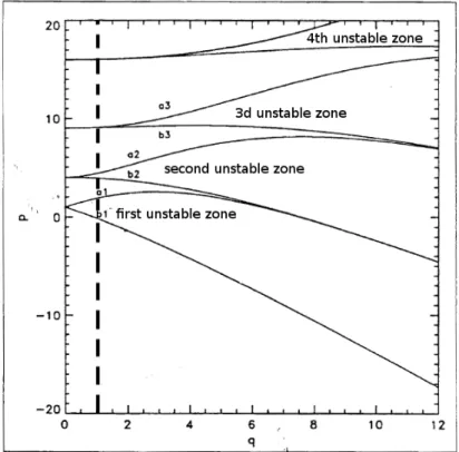
Mathieu equation

To explain the observations done during the simulations presented in next chapters especially second peak in the wave number spectrum, now we will briefly present ba-sics of Mathieu equation formalism. Let us consider one dimensional stationary wave which follows solution of Helmholtz equation (3.4). If fluctuations of plasma density or magnetic field are present, the wave refractive index is also perturbed. To investi-gate how each wave-number of the turbulence interacts with the probing wave, we will