Publisher’s version / Version de l'éditeur:
Proceedings of Combustion Institute, 33, pp. 601-608, 2011
READ THESE TERMS AND CONDITIONS CAREFULLY BEFORE USING THIS WEBSITE. https://nrc-publications.canada.ca/eng/copyright
Vous avez des questions? Nous pouvons vous aider. Pour communiquer directement avec un auteur, consultez la première page de la revue dans laquelle son article a été publié afin de trouver ses coordonnées. Si vous n’arrivez pas à les repérer, communiquez avec nous à [email protected].
Questions? Contact the NRC Publications Archive team at
[email protected]. If you wish to email the authors directly, please see the first page of the publication for their contact information.
NRC Publications Archive
Archives des publications du CNRC
This publication could be one of several versions: author’s original, accepted manuscript or the publisher’s version. / La version de cette publication peut être l’une des suivantes : la version prépublication de l’auteur, la version acceptée du manuscrit ou la version de l’éditeur.
For the publisher’s version, please access the DOI link below./ Pour consulter la version de l’éditeur, utilisez le lien DOI ci-dessous.
https://doi.org/10.1016/j.proci.2010.06.068
Access and use of this website and the material on it are subject to the Terms and Conditions set forth at
A numerical and experimental study of a laminar sooting coflow jet-A1
diffusion flame
Saffaripour, M.; Zabeti, P.; Dworkin, S. B.; Zhang, Q.; Thomson, M. J.; Guo,
H.; Liu, F.; Smallwood, G. J.
https://publications-cnrc.canada.ca/fra/droits
L’accès à ce site Web et l’utilisation de son contenu sont assujettis aux conditions présentées dans le site LISEZ CES CONDITIONS ATTENTIVEMENT AVANT D’UTILISER CE SITE WEB.
NRC Publications Record / Notice d'Archives des publications de CNRC:
https://nrc-publications.canada.ca/eng/view/object/?id=960ffc3c-e2c4-4390-9800-8f6ca520db06 https://publications-cnrc.canada.ca/fra/voir/objet/?id=960ffc3c-e2c4-4390-9800-8f6ca520db06Proceedings of Combustion Institute – Canadian Section Spring Technical Meeting Carleton University, Ottawa May 9-12, 2010
A Numerical and Experimental Study of a Laminar Sooting Coflow
Jet-A1 Diffusion Flame
M. Saffaripour
a, P. Zabeti
a, S. B. Dworkin
a, Q. Zhang
a, M. J. Thomson
a1, H. Guo
b, F. Liu
b,
G. J. Smallwood
ba Department of Mechanical and Industrial Engineering, University of Toronto, 5 King’s College Road, Toronto, Ontario, M5S 3G8, Canada
b Inst. for Chemical Process and Environmental Technology, National Research Council of Canada Building M-9, 1200 Montreal Road, Ottawa, Ontario, K1A 0R6, Canada
1. Introduction
Developing multidimensional flame models for blended liquid fuels, such as jet fuel, is challenging, mainly due to the very large chemical kinetic mechanisms and the associated computational resources required. Numerous researchers use a surrogate mixture to approximate the chemical and thermophysical properties of complex multicomponent blends. Honnet et al. [1] performed detailed calculations of an opposed jet diffusion flame using a surrogate mixture (80% n-decane and 20% 1,2,4-trimethylbenzene, by mass) and measured the soot volume fraction, autoignition, and extinction properties of both aviation kerosene and the surrogate. The results of the experiments for the surrogate and the actual jet fuel were reasonably close. The agreement between the numerical calculations using the detailed chemical kinetic mechanism of the surrogate, and the experiments were also satisfactory. Moss et
al. [2] implemented a flamelet-based two-equation soot model for a simple Jet-A surrogate, comprising 77% n-decane and 23% 1,3,5-trimethylbenzene by liquid volume, in a laminar coflow diffusion flame, and measured soot volume fraction, mixture fraction, and temperature. The radial soot volume fraction profiles and location of the peak concentration were predicted reasonably well. Wen et al. [3] modeled soot formation in a turbulent coflow non-premixed kerosene flame using a kerosene surrogate (20% toluene and 80% decane by liquid volume), a laminar flamelet approach, and the 141-chemical species mechanism of Dagaut et al. [4]. Comparisons were made for soot volume fraction and soot number density. After unsatisfactory initial comparisons, improvements were obtained in the results with a Polyaromatic Hydrocarbon (PAH)-based soot inception model as compared to an acetylene-based model.
Numerically solving multidimensional flames with detailed chemistry and transport proves to be a computationally intensive task, especially when complex fuels, such as jet fuel, are considered. Due to the inherently high computational cost of such models, parallel implementation has seen significant development in the last two decades. In 1991, Smooke and Giovangigli [5] presented a numerical simulation of a laminar coflow methane/air diffusion flame with 6 processors, using strip-domain decomposition. Since that time, numerous researchers have utilized a similar strip-domain decomposition strategy wherein subdomain boundaries are placed perpendicular to the axial flow direction. Zhang et al. [6,7] developed a detailed model for an ethylene/air coflow flame using a semi-implicit scheme and divided the computational domain into 16 subdomains. Flame temperatures, species concentrations, soot volume fraction, and soot number density compared well to experimental data in the literature. Dworkin et al. [8] presented a distributed-memory parallel computation of a time-dependent sooting ethylene/air coflow diffusion flame on 40 CPUs. Unlike most other parallel coflow laminar flame models, that study (like the present work) extended parallel simulation to the solution of a problem that was intractable by serial processing.
Although some common simplifications are used in the modeling component of the present study, such as the use of a surrogate fuel, axisymmetry, and confinement to the laminar regime, the present model seeks to retain a high level of quantitative accuracy including detailed chemistry, transport, soot formation, aerosol dynamics, radiation heat transfer, and fluid dynamics. The model builds upon the algorithms of Zhang et al. [6,7], first by increasing the parallelization/decomposition capabilities to 192 CPUs, and then by applying the model to a non-premixed laminar coflow flame of a Jet-A1 surrogate fuel. The present work then seeks to validate the model using experimental data for species and soot concentrations obtained using GC and laser extinction, respectively.
1
2
2. Burner Geometry and Experimental Techniques
A coannular burner is used in the present experimental study of the laminar coflow Jet-A1 diffusion flame (details available in [9]). Vaporization of heavy multi-component liquid fuels, such as Jet-A1 in the present study, is a significant challenge due to high boiling points (438 K – 538 K). To lower the required temperature for vaporization, the fuel is heavily diluted with nitrogen. Using a W-102A Bronkhorst vapour delivery system, a reproducible flame with reliable long-term stability was obtained. The fuel mixture is vaporized at 463 K and transferred to the burner via heated tubes maintained at 523 K. To prevent condensation of the fuel inside the burner, the coflow air is heated to 423 K and the last two inches of the fuel tube are kept at 473 K by thin flexible Minco heaters. The fuel and carrier gas flow rates are 11.2 g/hr and 710 mL/min (at 273 K), respectively. The volumetric flow rate of the coflow air is 55.0 L/min (at 294 K). Excess oxygen, with a flow rate of 3.0 L/min (at 294 K), is added to the coflow air to enable high dilution of the fuel stream without increasing the flame lift-off height. The mean velocities of the fuel and air streams are 20.34 cm/s and 21.89 cm/s, respectively, at the burner exit. The resulting visible flame height is 65 mm with a lift-off of about 2 mm. The soot concentration in the flame is such that it allows gaseous species sampling without clogging the probes, while providing a high enough extinction of the laser beam for accurate soot volume fraction measurements.
Sampling was conducted by continuously withdrawing gas from the flame using an Agilent deactivated fused silica GC column. The orifice diameter of the microprobe is 250 µm and the outer diameter is 350 µ m. The suction flow rate decreases from approximately 150 cm3/min to 20 cm3/min as the probe tip moves higher in the flame. This is due to the rise in temperature at higher locations in the flame. A diaphragm vacuum pump was used to extract the samples from the microprobe tip, along the heated tubing, through a filter, and propel them to a Varian 3800 series GC with a Flame Ionization Detector (FID), in series with a Varian 450 GC with a Thermal Conductivity Detector (TCD). The GC-FID was used to quantify levels of light hydrocarbons, and the GC-TCD was used to measure CO and CO2 concentrations in the gas samples. At z = 28 mm, the sampling probe would clog due to excessive amounts of soot accumulation at the probe tip. As a result, gas sampling was only conducted below this height. The accuracy of the gas sampling measurements is estimated to be ±15%.
A well-established Laser Extinction Measurement method (see, for example [9] and [10]), is used to determine the local soot volume fraction in the flame. The line integrated transmission is converted to the local extinction coefficient by the Three-Point Abel Inversion method [11]. Light scattering by the particles was assumed to be negligible (as is done for example, in [9] and [12]). Radial profiles of soot volume fraction at six axial locations and with a resolution of 0.2 mm are measured. 3000 readings are averaged over a 15 s period for each datum.
3. Numerical Model
3.1. Model Description
The target flame is the steady, atmospheric pressure, laminar sooting coflow Jet-A1 diffusion flame described in Section 2. The fully-coupled elliptic conservation equations for mass, momentum, energy, species mass fractions, soot aggregate number densities, and primary particle number densities are solved in a two-dimensional axisymmetric cylindrical coordinate system. A detailed description of the governing equations, boundary conditions and solution methodology can be found in [6,7,13].
The soot sectional model considers nucleation based on the collisions of two pyrene molecules in the free-molecular regime, surface growth, PAH surface condensation, coagulation, fragmentation, particle diffusion, and thermophoresis. The model is the same as that used by Zhang et al. [6,7] to model soot formation in an ethylene flame. No adjustments were made to parameters to fit the data as an objective was to evaluate how robust this soot model would be to changes in fuel. Each soot aggregate is assumed to be composed of equally-sized spherical primary particles and to have a constant fractal dimension of 1.8. The mass range of soot aggregates is divided logarithmically into thirty-five discrete sections, each with a prescribed representative mass [14]. The nucleation step connects the gaseous incipient species with the solid soot phase. Surface growth is calculated by the HACA mechanism developed in [15,16,17]. All parameters are kept as in [15] except for , the fraction of the soot surface that is available for surface reactions. Here, the temperature dependent of Xu et al. [18] is used (i.e., = 0.004exp[10800/T]).
The soot model accounts for PAH condensation by considering collisions between pyrene molecules and soot aggregates [15]. The probability of sticking in each collision, [19] is assumed to be 0.55 [13]. The source term in the energy equation due to the nongray radiative heat transfer by soot, H2O, CO2, and CO, is calculated using the discrete-ordinates method and a statistical narrow-band correlated-k-based model developed by Liu et al. [20].
3
3.2. Chemical Kinetic MechanismJet-A1 is a complex mixture of alkanes (50-65% by volume), aromatics (10-20% by volume) and cycloalkanes (20-30% by volume). Dagaut et al. [21] studied experimentally the oxidation kinetics of Jet-A1 in a Jet Stirred Reactor (JSR). A surrogate mixture, consisting of 69% decane, 20% propylbenzene, 11% n-propylcyclohexane (by mole), and a detailed chemical kinetic mechanism, consisting of 2027 reactions and 263 species, was used to model Jet-A1 in [21] and is used in the present study. This mechanism does not contain the reactions describing the growth of PAHs to pyrene, which is the soot precursor species in the present work. The chemical kinetic mechanism developed by Appel et al. [15] for the oxidation of C2 fuels, which includes the growth of PAHs up to pyrene, is thus also used in the present work. Therefore, the full chemical kinetic mechanism used here combines the mechanism from Dagaut et al. [21] for Jet-A1 oxidation with that of Appel et al. [15] for PAH growth and pyrene formation. The resulting combined mechanism considers 304 species and 2265 reactions.
3.3. Numerical Method
The computational domain extends 12.29 cm in the axial direction and 4.75 cm in the radial direction, and is divided into 192 (z) × 88 (r) control volumes. A non-uniform mesh is used to save computational cost while still resolving large spatial gradients. The grid is finest in the flame region with maximum resolutions of 0.02 cm between r = 0.0 cm and r = 0.8 cm in the radial direction, and 0.025 cm between z = 0.0 cm and z = 8.0 cm in the axial direction. Flat velocity profiles are assumed for the inlet fuel and oxidizer streams with values given in Section 2. The inlet temperatures for the fuel and oxidizer are set to 453 K and 373 K, respectively, based on measurements of the heated flow. Symmetry, free-slip, and zero-gradient conditions are enforced at the centerline, the outer radial boundary, and the outflow boundary, respectively.
As in previous works [6,7], the finite volume method is used to discretize the governing equations. A staggered mesh is used with a semi-implicit scheme to handle the pressure and velocity coupling and to solve the discretized equations [22]. The diffusive terms are discretized using a second-order central difference scheme while the convective terms are discretized using a power law scheme [22]. Pseudo-transient continuation is used to aid convergance from an arbitrary starting estimate. At each pseudo-time step, the gaseous species equations are solved in a coupled manner at each control volume to effectively deal with the stiffness of the system and speedup the convergence process [23]. After iteration of the species equations, the soot equations are also solved simultaneously. The thermal properties of the gaseous species and chemical reaction rates are obtained using CHEMKIN subroutines [24,25]. Transport properties which include mixture-averaged quantities for viscosities, conductivities, and diffusion coefficients, as well as thermal diffusion coefficients for H and H2, are evaluated using TPLIB [26,27].
Due to the immense computational intensity of the problem, solution would be intractable with serial processing. Therefore, distributed-memory parallelization with strip-domain decomposition is employed. The computational domain is divided uniformly into 192 subdomains with the boundaries of each subdomain perpendicular to the z-axis. The algorithm uses the Message Passing Interface library to parallelize the code [28,29]. The computations are performed on the Tightly Coupled System of SciNet, on three 64-core power 6 nodes with 4.7 GHz chip speeds. Each iteration takes approximately 73 seconds, and approximately 25000 iterations are required for the solution to converge from an arbitrary starting estimate.
4. Results and Discussion
The left panel of Fig. 1 depicts the computed temperature isotherms and the right panel of Fig. 1 depicts the computed isopleths of soot volume fraction. The maximum flame temperature is computed as 1895 K, and the flame lift-off (defined as the lowest point in the flame hotter than 500 K) is 2 mm above the burner surface. The maximum soot volume fraction is predicted as 5.5 ppm occurring on the wings of the flame at z = 35 mm. The sharp decay in soot volume fraction at z = 55 mm (where T~1800 K) indicates that the calculated visible flame height is fairly close to the experimentally observed flame height of 65 mm.
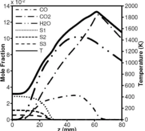
Figure 2 shows the computed centerline mole fraction profiles of CO, CO2, H2O, surrogate components n-decane (S1), n-propylbenzene (S2), n-propylcyclohexane (S3), and temperature (T). It can be seen that along the centerline, at approximately z = 30 mm, all three components of the surrogate are completely consumed. At this point in the flame, the model predicts sharp rises in CO2 and H2O mole fractions, and in temperature. The peak in temperature and the main combustion product CO2 occur at approximately z = 60 mm, which is also consistent with the experimentally observed flame height. The sharp consumption of CO, between z = 50 mm and z = 62 mm, suggests that hydrocarbon species still exist in the flame up to this point.
4
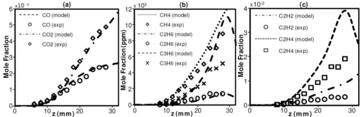
In the present study, computed and measured axial centerline concentration profiles of some major species are compared. The experimental results from GC-FID and TCD show that the major intermediate combustion products were CO, CO2, methane (CH4), acetylene (C2H2), ethylene (C2H4), ethane (C2H6), and propylene (C3H6). The experimental data are averaged over three trials. The plots in Fig. 3(a), 3(b), and 3(c) display the comparisons between model predictions and experimental measurements for these species. As can be seen from Fig. 3(a), the model predicts CO and CO2 concentrations very accurately up to z = 28 mm. Figure 3(b) also demonstrates excellent agreement between the model predictions and experimental data for CH4, C2H6 and C3H6. Figure 3(c) illustrates that the model slightly overpredicts C2H2 and C2H4 concentrations, especially above z = 15 mm, where model predictions start to deviate from experimental data. This may be caused by differences between the surrogate and actual fuel, or by inaccuracies in the gas phase chemistry. It should be noted that the differences between the measurements and the model in the present work, are in line with those observed in [21].
The computed soot volume fraction radial profiles are compared to the measurements at three axial heights above the burner,
z = 31 mm, z = 41 mm, and z = 51 mm, in Figs. 4(a), 4(b), and 4(c), respectively. It can be seen from Fig. 4(a) that the general shape and order of magnitude of the soot profile is well predicted by the model at
z = 31 mm. The model predicts a peak value of 5.33 ppm, which compares well to the peak measured value of 3.72 ppm. The model predicts a peak location somewhat further away from the centerline than was measured. Larger discrepancies, however, arise above this height as seen at z = 41 mm (Fig. 4(b)) and at z = 51 mm (Fig. 4(c)). At z = 41 mm, measured soot volume fraction has increased along the centerline and the peak is moving radially inward. The model fails to predict both of these features although the magnitude of soot volume fraction along the wings is well reproduced. At z = 51 mm, measured soot volume fraction peaks at 7.0 ppm near the centerline and monotonically decreases outward. The model fails to predict this trend, showing almost no soot along the centerline at this height. The significant underprediction of soot concentration on the centerline has been observed previously (see, for example [6,7,30,31]). More insight into this discrepancy can be gained from Fig. 4(d), which shows the maximum soot volume fraction as a function of axial height for the model and the experiment. The model predicts a sharp decrease starting near z = 35 mm, whereas in the experiment, this decrease does not occur until approximately z = 50 mm. Although the model predicts the correct order of magnitude of soot volume fraction, the profile is considerably shorter. The discrepancy is magnified between z = 50 mm and z = 60 mm, at which point the sharp decrease in soot volume fraction has been predicted in the model, but has not yet occurred in the experiment. Above z = 35 mm, the location of peak soot is at the center of the flame and is significantly underpredicted by the model. At z = 51 mm (Fig. 4(c)) this is seen as a significant deviation from the experimental data in centerline soot concentration, however, the model correctly predicts the oxidation of soot along the wings, as evidenced by the agreement between model and experiment at radial locations greater than r = 22 mm.
These results are quite promising given the fact that the PAH growth model was taken from a C2 mechanism and its applicability to jet fuel had not been tested. In addition, the soot model parameters are not adjusted to fit the experimental data and there is considerable room for improvement in the numerical model. One such improvement would be the consideration of higher order transport effects, which are generally thought to be important in mixtures with large molecular weight disparities such as jet fuel/air [32].
Fig. 1 Left panel: Computed isotherms. Right panel: Computed isopleths of soot volume fraction. r (cm) z (c m ) -1 0 1 0 1 2 3 4 5 6 7380 850 1320 1790 1895 K 373 K r (cm) -1 0 1 0 1 2 3 4 5 6 7 0.05 2.3 4.55 5.45 ppm 0.0 ppm
Fig. 2 Computed centerline mole fraction profiles of CO, CO2, H2O, surrogate
components n-decane (S1), n-propylbenzene (S2), n-propylcyclohexane (S3), and temperature (T).
5
Fig. 3 (a) Computational (model) and Experimental (exp) comparison of CO and CO2 mole fractions along the flame
centerline. (b) Computational (model) and Experimental (exp) comparison of CH4, C2H6, and C3H6 mole fractions along the
flame centerline. (c) Computational (model) and Experimental (exp) comparison of C2H2, and C2H4 mole fractions along the
flame centerline.
Fig. 4 Computational end experimental soot volume fraction radial profiles at (a) z = 31 mm, (b) z = 41 mm, and (c) z = 51mm. (d) Computational and experimental maximum soot volume fractions as a function of flame height.
5. Conclusions and Future Work
A laminar sooting coflow Jet-A1 diffusion flame is numerically simulated, using a 3-component surrogate fuel and detailed chemistry and transport, in parallel over 192 CPUs. A detailed PAH-based sectional soot model describes soot formation. All soot model parameters were kept the same as in previous ethylene flame models. Measurements of gaseous species concentrations and soot volume fraction are performed on a coflow flame of vaporized Jet-A1, heavily diluted with nitrogen. A comparison between the measured results and model predictions reveals good agreement for centerline species concentrations. The soot volume fraction along the wings and at the lower radial profiles were well predicted and reproduced within the correct order of magnitude; however, this model, like others underpredicts soot concentration on the centerline.
This work shows that parallelization and substantial computing power enable the solution of a coflow jet fuel diffusion flame with detailed chemistry, transport, and soot formation. The results suggest that the detailed soot model and its model constants may be independent of the specific fuel used. This is encouraging; however, further work is needed to study sooting flames with other fuels. The current study and many others have noted the underprediction of soot along the centerline. This is an area in particular need of progress. Further experimental work is needed to measure flame temperature, radial species profiles including aromatics, and soot morphological properties within the flame. This data would assist in further validating the model and in helping to resolve discrepancies in the soot model.
6. Acknowledgements
The authors acknowledge the Natural Sciences and Engineering Research Council of Canada for financial support, Dr. Philippe Dagaut for providing the jet fuel mechanism, Dr. Mani Sarathy and Dr. Kevin Thomson for help with the experimental setup, the National Research Council of Canada for providing jet fuel samples, and the SciNet Consortium for providing the computational resources.
Reference
[1] S. Honnet, K. Seshadri, U. Niemann, N. Peters, Proc. Combust. Inst., 32 (2009) 485-492. [2] J.B. Moss, I.M. Aksit, Proc. Combust. Inst., 31 (2007) 3139-3149.
6
[4] P. Dagaut, Phys. Chem. Chem. Phys., 4 (2002) 2079-2094.
[5] M.D. Smooke, V. Giovangigli, Int. J. Supercomp. Appl., 5 (1991) 34-49.
[6] Q. Zhang, H. Guo, F. Liu, G.J. Smallwood, M.J. Thomson, Proc. Combust. Inst., 32 (2009) 761-768. [7] Q. Zhang, M.J. Thomson, H. Guo, F. Liu, G.J. Smallwood, Combust. Flame, 156 (3) (2009) 697-705. [8] S.B. Dworkin, J.A. Cooke, B.A.V. Bennett, M.D. Smooke, R. J. Hall, M.B. Colket, Combust. Theor.
Model., 13 (5) (2009) 795-822.
[9] D.R. Snelling, K.A. Thomson, G.J. Smallwood, O.L. Gülder, Appl. Optics, 38 (12) (1999) 2478-2485. [10] K.A. Thomson, O.L. Gülder, E.J. Weckman, R.A. Fraser, G.J. Smallwood, D.R. Snelling, Combust. Flame,
140 (2005) 222-232.
[11] C.J. Dasch, Appl. Optics, 31 (8) (1992) 1146-1152.
[12] P.S. Greenberg, J.C. Ku, Appl. Optics, 36 (22) (1997) 5514-552.
[13] Q. Zhang, Detailed Modeling of Soot Formation/Oxidation in Laminar Coflow Diffusion Flames, PhD Thesis, University of Toronto, Toronto, Canada, 2009.
[14] S.H. Park, S.N. Rogak, W.K. Bushe, J.Z. Wen, M.J. Thomson, Combust. Theor. Model., 9 (2005) 499-513. [15] J. Appel, H. Bockhorn, M. Frenklach, Combust. Flame, 121 (2000) 122-136.
[16] S.J. Harris, A.M. Weiner, Combust. Sci. Technol., 38 (1984) 75-84.
[17] K.G. Neoh, J.B. Howard, A.F. Sarofim, Soot oxidation in flames, in Particulate Carbon: Formation During Combustion, Plenum, New York, 1981.
[18] P.B. Sunderland, G.M. Faeth, F. Xu, Combust. Flame, 108 (1997) 471-493. [19] D.F. Kronholm, J.B. Howard, Proc. Combust. Inst., 28 (2000) 2555-2561.
[20] F. Liu, G.J. Smallwood, O.L. Gülder, J. Thermophys. Heat Transfer, 14 (2) (2000) 278-281. [21] P. Dagaut, S. Gaïl, J. Phys. Chem., 111 (2007) 3992-4000.
[22] S.V. Patanker, Numerical Heat Transfer and Fluid Flow, Hemisphere, New York, 1980.
[23] Z. Liu, C. Liao, C. Liu, S. McCormick, 33rd Aerospace Sciences Meeting and Exhibit, Reno, 1995.
[24] R.J. Kee, J.A. Miller, T.H. Jefferson, Chemkin: A General Purpose, Problem Independent, Transportable, Fortran Chemical Kinetics Code Package, Report SAND80-8003, 1980.
[25] R.J. Kee, F.M. Rupley, J.A. Miller, A Fortran chemical kinetics package for the analysis of gas-phase chemical kinetics, Sandia Report SAND89-8009, 1989.
[26] R.J. Kee, J. Warnatz, J.A. Miller, A Fortran Computer Code Package for the Evaluation of Gas-Phase Viscosities, Conductivities, and Diffusion Coefficients, Report SAND82-8209, 1983.
[27] R.J. Kee, G. Dixon-Lewis, J. Warnatz, M.E. Coltrin, J.A. Miller, A Fortran Computer Code Package for the Evaluation of Gas-Phase Multicomponent Transport Properties, Report SAND86-8246, 1986.
[28] M. Snir, S. Otto, S. Huss-Lederman, D. Walker, J. Dongarra, MPI: The Complete Reference Volume 1, MIT Press, Cambridge, MA, 1998.
[29] W. Gropp, S. Huss-Lederman, A. Lumsdaine, E. Lusk, B. Nitzberg, W. Saphir, M. Snir, MPI: The Complete Reference Volume 2, MIT Press, Cambridge , MA, 1998.
[30] I.M. Kennedy, C. Yam, D.C. Rapp, R.J. Santoro, Combust. Flame, 107 (1996) 368-382.
[31] M.D. Smooke, C.S. McEnally, L.D. Pfefferle, R.J. Hall, M.B. Colket, Combust. Flame, 117 (1999) 117-139. [32] S.B. Dworkin, V. Giovangigli, M.D. Smooke, Proc. Combust. Inst., 32 (1) (2009) 1165-1172.