Measurement of the t$\bar t$ production cross section in $\bar p$p collisions at $\sqrt s$ = 1.96 TeV using secondary vertex b tagging

arXiv:hep-ex/0611002v2 2 Feb 2007

Measurement of the tt production cross section in p¯

p

collisions at

√

s

= 1.96 TeV

using secondary vertex b tagging

V.M. Abazov,35 B. Abbott,75 M. Abolins,65 B.S. Acharya,28 M. Adams,51 T. Adams,49 E. Aguilo,5 S.H. Ahn,30 M. Ahsan,59 _{G.D. Alexeev,}35 _{G. Alkhazov,}39 _{A. Alton,}64 _{G. Alverson,}63 _{G.A. Alves,}2 _{M. Anastasoaie,}34

L.S. Ancu,34 _{T. Andeen,}53 _{S. Anderson,}45_{B. Andrieu,}16 _{M.S. Anzelc,}53 _{Y. Arnoud,}13 _{M. Arov,}52_{A. Askew,}49

B. ˚Asman,40_{A.C.S. Assis Jesus,}3_{O. Atramentov,}49 _{C. Autermann,}20 _{C. Avila,}7_{C. Ay,}23 _{F. Badaud,}12_{A. Baden,}61

L. Bagby,52_{B. Baldin,}50 _{D.V. Bandurin,}59 _{P. Banerjee,}28 _{S. Banerjee,}28 _{E. Barberis,}63 _{P. Bargassa,}80

P. Baringer,58 _{C. Barnes,}43 _{J. Barreto,}2 _{J.F. Bartlett,}50 _{U. Bassler,}16 _{D. Bauer,}43 _{S. Beale,}5 _{A. Bean,}58

M. Begalli,3_{M. Begel,}71 _{C. Belanger-Champagne,}40_{L. Bellantoni,}50 _{A. Bellavance,}67 _{J.A. Benitez,}65 _{S.B. Beri,}26

G. Bernardi,16 _{R. Bernhard,}41_{L. Berntzon,}14 _{I. Bertram,}42_{M. Besan¸con,}17 _{R. Beuselinck,}43 _{V.A. Bezzubov,}38

P.C. Bhat,50 _{V. Bhatnagar,}26 _{M. Binder,}24_{C. Biscarat,}19_{I. Blackler,}43 _{G. Blazey,}52 _{F. Blekman,}43 _{S. Blessing,}49

D. Bloch,18 _{K. Bloom,}67 _{U. Blumenschein,}22 _{A. Boehnlein,}50 _{T.A. Bolton,}59 _{G. Borissov,}42 _{K. Bos,}33 _{T. Bose,}77

A. Brandt,78_{R. Brock,}65 _{G. Brooijmans,}70_{A. Bross,}50_{D. Brown,}78 _{N.J. Buchanan,}49 _{D. Buchholz,}53_{M. Buehler,}81

V. Buescher,22 _{S. Burdin,}50 _{S. Burke,}45 _{T.H. Burnett,}82_{E. Busato,}16_{C.P. Buszello,}43 _{J.M. Butler,}62 _{P. Calfayan,}24

S. Calvet,14 _{J. Cammin,}71 _{S. Caron,}33 _{W. Carvalho,}3 _{B.C.K. Casey,}77_{N.M. Cason,}55 _{H. Castilla-Valdez,}32

S. Chakrabarti,17 _{D. Chakraborty,}52 _{K.M. Chan,}71 _{A. Chandra,}48 _{F. Charles,}18_{E. Cheu,}45 _{F. Chevallier,}13

D.K. Cho,62 _{S. Choi,}31 _{B. Choudhary,}27 _{L. Christofek,}77 _{D. Claes,}67_{B. Cl´ement,}18 _{C. Cl´ement,}40 _{Y. Coadou,}5

M. Cooke,80 _{W.E. Cooper,}50 _{D. Coppage,}58_{M. Corcoran,}80 _{F. Couderc,}17 _{M.-C. Cousinou,}14 _{B. Cox,}44

S. Cr´ep´e-Renaudin,13_{D. Cutts,}77_{M. ´Cwiok,}29_{H. da Motta,}2_{A. Das,}62_{M. Das,}60_{B. Davies,}42_{G. Davies,}43_{K. De,}78

P. de Jong,33 _{S.J. de Jong,}34 _{E. De La Cruz-Burelo,}64_{C. De Oliveira Martins,}3_{J.D. Degenhardt,}64 _{F. D´eliot,}17

M. Demarteau,50_{R. Demina,}71 _{D. Denisov,}50_{S.P. Denisov,}38_{S. Desai,}50 _{H.T. Diehl,}50 _{M. Diesburg,}50_{M. Doidge,}42

A. Dominguez,67 _{H. Dong,}72 _{L.V. Dudko,}37 _{L. Duflot,}15 _{S.R. Dugad,}28 _{D. Duggan,}49 _{A. Duperrin,}14 _{J. Dyer,}65

A. Dyshkant,52 _{M. Eads,}67 _{D. Edmunds,}65 _{J. Ellison,}48_{J. Elmsheuser,}24 _{V.D. Elvira,}50 _{Y. Enari,}77 _{S. Eno,}61

P. Ermolov,37 _{H. Evans,}54 _{A. Evdokimov,}36 _{V.N. Evdokimov,}38 _{L. Feligioni,}62_{A.V. Ferapontov,}59 _{T. Ferbel,}71

F. Fiedler,24 F. Filthaut,34 W. Fisher,50 H.E. Fisk,50 I. Fleck,22 M. Ford,44 M. Fortner,52 H. Fox,22 S. Fu,50 S. Fuess,50 _{T. Gadfort,}82 _{C.F. Galea,}34 _{E. Gallas,}50_{E. Galyaev,}55_{C. Garcia,}71_{A. Garcia-Bellido,}82_{J. Gardner,}58

V. Gavrilov,36_{A. Gay,}18_{P. Gay,}12_{W. Geist,}18 _{D. Gel´e,}18_{R. Gelhaus,}48_{C.E. Gerber,}51_{Y. Gershtein,}49_{D. Gillberg,}5

G. Ginther,71 N. Gollub,40 B. G´omez,7 A. Goussiou,55 P.D. Grannis,72 H. Greenlee,50 Z.D. Greenwood,60 E.M. Gregores,4_{G. Grenier,}19 _{Ph. Gris,}12 _{J.-F. Grivaz,}15_{A. Grohsjean,}24_{S. Gr¨unendahl,}50 _{M.W. Gr¨unewald,}29

F. Guo,72 _{J. Guo,}72 _{G. Gutierrez,}50_{P. Gutierrez,}75 _{A. Haas,}70_{N.J. Hadley,}61_{P. Haefner,}24 _{S. Hagopian,}49

J. Haley,68 I. Hall,75R.E. Hall,47 L. Han,6 K. Hanagaki,50P. Hansson,40 K. Harder,59 A. Harel,71R. Harrington,63 J.M. Hauptman,57 _{R. Hauser,}65_{J. Hays,}43 _{T. Hebbeker,}20 _{D. Hedin,}52 _{J.G. Hegeman,}33 _{J.M. Heinmiller,}51

A.P. Heinson,48 _{U. Heintz,}62 _{C. Hensel,}58_{K. Herner,}72_{G. Hesketh,}63 _{M.D. Hildreth,}55 _{R. Hirosky,}81_{J.D. Hobbs,}72

B. Hoeneisen,11 H. Hoeth,25 M. Hohlfeld,15 S.J. Hong,30 R. Hooper,77 P. Houben,33 Y. Hu,72 Z. Hubacek,9 V. Hynek,8 _{I. Iashvili,}69_{R. Illingworth,}50_{A.S. Ito,}50_{S. Jabeen,}62_{M. Jaffr´e,}15 _{S. Jain,}75 _{K. Jakobs,}22 _{C. Jarvis,}61

A. Jenkins,43_{R. Jesik,}43 _{K. Johns,}45 _{C. Johnson,}70_{M. Johnson,}50 _{A. Jonckheere,}50_{P. Jonsson,}43 _{A. Juste,}50

D. K¨afer,20 _{S. Kahn,}73 _{E. Kajfasz,}14 _{A.M. Kalinin,}35 _{J.M. Kalk,}60_{J.R. Kalk,}65 _{S. Kappler,}20 _{D. Karmanov,}37

J. Kasper,62 _{P. Kasper,}50_{I. Katsanos,}70_{D. Kau,}49 _{R. Kaur,}26_{R. Kehoe,}79 _{S. Kermiche,}14 _{N. Khalatyan,}62

A. Khanov,76_{A. Kharchilava,}69_{Y.M. Kharzheev,}35_{D. Khatidze,}70_{H. Kim,}78 _{T.J. Kim,}30 _{M.H. Kirby,}34_{B. Klima,}50

J.M. Kohli,26 _{J.-P. Konrath,}22 _{M. Kopal,}75 _{V.M. Korablev,}38 _{J. Kotcher,}73 _{B. Kothari,}70 _{A. Koubarovsky,}37

A.V. Kozelov,38 _{D. Krop,}54 _{A. Kryemadhi,}81 _{T. Kuhl,}23 _{A. Kumar,}69 _{S. Kunori,}61_{A. Kupco,}10 _{T. Kurˇca,}19

J. Kvita,8 _{D. Lam,}55_{S. Lammers,}70 _{G. Landsberg,}77 _{J. Lazoflores,}49 _{A.-C. Le Bihan,}18 _{P. Lebrun,}19_{W.M. Lee,}52

A. Leflat,37 _{F. Lehner,}41 _{V. Lesne,}12 _{J. Leveque,}45 _{P. Lewis,}43 _{J. Li,}78 _{L. Li,}48 _{Q.Z. Li,}50 _{J.G.R. Lima,}52

D. Lincoln,50 _{J. Linnemann,}65_{V.V. Lipaev,}38 _{R. Lipton,}50_{Z. Liu,}5 _{L. Lobo,}43_{A. Lobodenko,}39_{M. Lokajicek,}10

A. Lounis,18 _{P. Love,}42_{H.J. Lubatti,}82 _{M. Lynker,}55_{A.L. Lyon,}50 _{A.K.A. Maciel,}2 _{R.J. Madaras,}46_{P. M¨attig,}25

C. Magass,20_{A. Magerkurth,}64_{A.-M. Magnan,}13_{N. Makovec,}15 _{P.K. Mal,}55 _{H.B. Malbouisson,}3 _{S. Malik,}67

V.L. Malyshev,35_{H.S. Mao,}50 _{Y. Maravin,}59_{M. Martens,}50 _{R. McCarthy,}72_{D. Meder,}23 _{A. Melnitchouk,}66

A. Mendes,14_{L. Mendoza,}7_{M. Merkin,}37 _{K.W. Merritt,}50_{A. Meyer,}20_{J. Meyer,}21_{M. Michaut,}17 _{H. Miettinen,}80

T. Millet,19 _{J. Mitrevski,}70 _{J. Molina,}3 _{R.K. Mommsen,}44 _{N.K. Mondal,}28 _{J. Monk,}44 _{R.W. Moore,}5_{T. Moulik,}58

G.S. Muanza,19_{M. Mulders,}50_{M. Mulhearn,}70_{O. Mundal,}22_{L. Mundim,}3 _{E. Nagy,}14_{M. Naimuddin,}27_{M. Narain,}62

T. Nunnemann,24_{V. O’Dell,}50_{D.C. O’Neil,}5 _{G. Obrant,}39_{C. Ochando,}15 _{V. Oguri,}3_{N. Oliveira,}3_{D. Onoprienko,}59

N. Oshima,50_{J. Osta,}55 _{R. Otec,}9 _{G.J. Otero y Garz´on,}51 _{M. Owen,}44 _{P. Padley,}80 _{N. Parashar,}56_{S.-J. Park,}71

S.K. Park,30 _{J. Parsons,}70_{R. Partridge,}77_{N. Parua,}72 _{A. Patwa,}73 _{G. Pawloski,}80_{P.M. Perea,}48 _{K. Peters,}44

P. P´etroff,15 _{M. Petteni,}43 _{R. Piegaia,}1 _{J. Piper,}65 _{M.-A. Pleier,}21 _{P.L.M. Podesta-Lerma,}32_{V.M. Podstavkov,}50

Y. Pogorelov,55_{M.-E. Pol,}2 _{A. Pompoˇs,}75 _{B.G. Pope,}65 _{A.V. Popov,}38 _{C. Potter,}5_{W.L. Prado da Silva,}3

H.B. Prosper,49_{S. Protopopescu,}73 _{J. Qian,}64 _{A. Quadt,}21 _{B. Quinn,}66 _{M.S. Rangel,}2 _{K.J. Rani,}28 _{K. Ranjan,}27

P.N. Ratoff,42 _{P. Renkel,}79_{S. Reucroft,}63 _{M. Rijssenbeek,}72 _{I. Ripp-Baudot,}18_{F. Rizatdinova,}76 _{S. Robinson,}43

R.F. Rodrigues,3 C. Royon,17 P. Rubinov,50 R. Ruchti,55 V.I. Rud,37 G. Sajot,13 A. S´anchez-Hern´andez,32 M.P. Sanders,16 _{A. Santoro,}3 _{G. Savage,}50_{L. Sawyer,}60 _{T. Scanlon,}43 _{D. Schaile,}24 _{R.D. Schamberger,}72

Y. Scheglov,39 _{H. Schellman,}53 _{P. Schieferdecker,}24 _{C. Schmitt,}25 _{C. Schwanenberger,}44 _{A. Schwartzman,}68

R. Schwienhorst,65 _{J. Sekaric,}49 _{S. Sengupta,}49 _{H. Severini,}75 _{E. Shabalina,}51 _{M. Shamim,}59 _{V. Shary,}17

A.A. Shchukin,38 _{R.K. Shivpuri,}27 _{D. Shpakov,}50_{V. Siccardi,}18 _{R.A. Sidwell,}59 _{V. Simak,}9 _{V. Sirotenko,}50

P. Skubic,75 _{P. Slattery,}71 _{R.P. Smith,}50 _{G.R. Snow,}67 _{J. Snow,}74 _{S. Snyder,}73_{S. S¨oldner-Rembold,}44 _{X. Song,}52

L. Sonnenschein,16 _{A. Sopczak,}42_{M. Sosebee,}78_{K. Soustruznik,}8 _{M. Souza,}2 _{B. Spurlock,}78_{J. Stark,}13_{J. Steele,}60

V. Stolin,36 _{A. Stone,}51 _{D.A. Stoyanova,}38_{J. Strandberg,}64 _{S. Strandberg,}40 _{M.A. Strang,}69 _{M. Strauss,}75

R. Str¨ohmer,24 _{D. Strom,}53_{M. Strovink,}46_{L. Stutte,}50 _{S. Sumowidagdo,}49 _{P. Svoisky,}55_{A. Sznajder,}3 _{M. Talby,}14

P. Tamburello,45 _{W. Taylor,}5 _{P. Telford,}44 _{J. Temple,}45 _{B. Tiller,}24 _{M. Titov,}22 _{V.V. Tokmenin,}35_{M. Tomoto,}50

T. Toole,61 _{I. Torchiani,}22 _{T. Trefzger,}23_{S. Trincaz-Duvoid,}16 _{D. Tsybychev,}72 _{B. Tuchming,}17 _{C. Tully,}68

P.M. Tuts,70 _{R. Unalan,}65_{L. Uvarov,}39_{S. Uvarov,}39 _{S. Uzunyan,}52_{B. Vachon,}5 _{P.J. van den Berg,}33_{B. van Eijk,}34

R. Van Kooten,54 _{W.M. van Leeuwen,}33 _{N. Varelas,}51 _{E.W. Varnes,}45 _{A. Vartapetian,}78 _{I.A. Vasilyev,}38

M. Vaupel,25P. Verdier,19 L.S. Vertogradov,35M. Verzocchi,50F. Villeneuve-Seguier,43 P. Vint,43 J.-R. Vlimant,16 E. Von Toerne,59 _{M. Voutilainen,}67,† _{M. Vreeswijk,}33_{H.D. Wahl,}49_{L. Wang,}61_{M.H.L.S Wang,}50 _{J. Warchol,}55

G. Watts,82 _{M. Wayne,}55_{G. Weber,}23 _{M. Weber,}50 _{H. Weerts,}65 _{N. Wermes,}21 _{M. Wetstein,}61 _{A. White,}78

D. Wicke,25 G.W. Wilson,58 S.J. Wimpenny,48 M. Wobisch,50 J. Womersley,50D.R. Wood,63 T.R. Wyatt,44 Y. Xie,77 _{S. Yacoob,}53 _{R. Yamada,}50 _{M. Yan,}61 _{T. Yasuda,}50 _{Y.A. Yatsunenko,}35 _{K. Yip,}73 _{H.D. Yoo,}77

S.W. Youn,53 _{C. Yu,}13 _{J. Yu,}78 _{A. Yurkewicz,}72 _{A. Zatserklyaniy,}52_{C. Zeitnitz,}25 _{D. Zhang,}50 _{T. Zhao,}82

B. Zhou,64 _{J. Zhu,}72 _{M. Zielinski,}71 _{D. Zieminska,}54 _{A. Zieminski,}54 _{V. Zutshi,}52 _{and E.G. Zverev}37

(DØ Collaboration)

1_{Universidad de Buenos Aires, Buenos Aires, Argentina} 2_{LAFEX, Centro Brasileiro de Pesquisas F´ısicas, Rio de Janeiro, Brazil}

3_{Universidade do Estado do Rio de Janeiro, Rio de Janeiro, Brazil} 4_{Instituto de F´ısica Te´orica, Universidade Estadual Paulista, S˜ao Paulo, Brazil}

5_{University of Alberta, Edmonton, Alberta, Canada, Simon Fraser University, Burnaby, British Columbia, Canada,}

York University, Toronto, Ontario, Canada, and McGill University, Montreal, Quebec, Canada

6_{University of Science and Technology of China, Hefei, People’s Republic of China} 7_{Universidad de los Andes, Bogot´a, Colombia}

8_{Center for Particle Physics, Charles University, Prague, Czech Republic} 9_{Czech Technical University, Prague, Czech Republic}

10_{Center for Particle Physics, Institute of Physics, Academy of Sciences of the Czech Republic, Prague, Czech Republic} 11_{Universidad San Francisco de Quito, Quito, Ecuador}

12_{Laboratoire de Physique Corpusculaire, IN2P3-CNRS, Universit´e Blaise Pascal, Clermont-Ferrand, France} 13_{Laboratoire de Physique Subatomique et de Cosmologie, IN2P3-CNRS, Universite de Grenoble 1, Grenoble, France}

14_{CPPM, IN2P3-CNRS, Universit´e de la M´editerran´ee, Marseille, France} 15_{IN2P3-CNRS, Laboratoire de l’Acc´el´erateur Lin´eaire, Orsay, France} 16_{LPNHE, IN2P3-CNRS, Universit´es Paris VI and VII, Paris, France} 17_{DAPNIA/Service de Physique des Particules, CEA, Saclay, France}

18_{IPHC, IN2P3-CNRS, Universit´e Louis Pasteur, Strasbourg, France, and Universit´e de Haute Alsace, Mulhouse, France} 19_{Institut de Physique Nucl´eaire de Lyon, IN2P3-CNRS, Universit´e Claude Bernard, Villeurbanne, France}

20_{III. Physikalisches Institut A, RWTH Aachen, Aachen, Germany} 21_{Physikalisches Institut, Universit¨at Bonn, Bonn, Germany} 22_{Physikalisches Institut, Universit¨at Freiburg, Freiburg, Germany}

23_{Institut f¨ur Physik, Universit¨at Mainz, Mainz, Germany} 24_{Ludwig-Maximilians-Universit¨at M¨unchen, M¨unchen, Germany} 25_{Fachbereich Physik, University of Wuppertal, Wuppertal, Germany}

26_{Panjab University, Chandigarh, India} 27_{Delhi University, Delhi, India}

28_{Tata Institute of Fundamental Research, Mumbai, India} 29_{University College Dublin, Dublin, Ireland} 30_{Korea Detector Laboratory, Korea University, Seoul, Korea}

31_{SungKyunKwan University, Suwon, Korea} 32_{CINVESTAV, Mexico City, Mexico}

33_{FOM-Institute NIKHEF and University of Amsterdam/NIKHEF, Amsterdam, The Netherlands} 34_{Radboud University Nijmegen/NIKHEF, Nijmegen, The Netherlands}

35_{Joint Institute for Nuclear Research, Dubna, Russia} 36_{Institute for Theoretical and Experimental Physics, Moscow, Russia}

37_{Moscow State University, Moscow, Russia} 38_{Institute for High Energy Physics, Protvino, Russia} 39_{Petersburg Nuclear Physics Institute, St. Petersburg, Russia}

40_{Lund University, Lund, Sweden, Royal Institute of Technology and Stockholm University, Stockholm, Sweden, and}

Uppsala University, Uppsala, Sweden

41_{Physik Institut der Universit¨at Z¨urich, Z¨urich, Switzerland} 42_{Lancaster University, Lancaster, United Kingdom}

43_{Imperial College, London, United Kingdom} 44_{University of Manchester, Manchester, United Kingdom}

45_{University of Arizona, Tucson, Arizona 85721, USA}

46_{Lawrence Berkeley National Laboratory and University of California, Berkeley, California 94720, USA} 47_{California State University, Fresno, California 93740, USA}

48_{University of California, Riverside, California 92521, USA} 49_{Florida State University, Tallahassee, Florida 32306, USA} 50_{Fermi National Accelerator Laboratory, Batavia, Illinois 60510, USA}

51_{University of Illinois at Chicago, Chicago, Illinois 60607, USA} 52_{Northern Illinois University, DeKalb, Illinois 60115, USA}

53_{Northwestern University, Evanston, Illinois 60208, USA} 54_{Indiana University, Bloomington, Indiana 47405, USA} 55_{University of Notre Dame, Notre Dame, Indiana 46556, USA}

56_{Purdue University Calumet, Hammond, Indiana 46323, USA} 57_{Iowa State University, Ames, Iowa 50011, USA} 58_{University of Kansas, Lawrence, Kansas 66045, USA} 59_{Kansas State University, Manhattan, Kansas 66506, USA} 60_{Louisiana Tech University, Ruston, Louisiana 71272, USA} 61_{University of Maryland, College Park, Maryland 20742, USA}

62_{Boston University, Boston, Massachusetts 02215, USA} 63_{Northeastern University, Boston, Massachusetts 02115, USA}

64_{University of Michigan, Ann Arbor, Michigan 48109, USA} 65_{Michigan State University, East Lansing, Michigan 48824, USA}

66_{University of Mississippi, University, Mississippi 38677, USA} 67_{University of Nebraska, Lincoln, Nebraska 68588, USA} 68_{Princeton University, Princeton, New Jersey 08544, USA} 69_{State University of New York, Buffalo, New York 14260, USA}

70_{Columbia University, New York, New York 10027, USA} 71_{University of Rochester, Rochester, New York 14627, USA} 72_{State University of New York, Stony Brook, New York 11794, USA}

73_{Brookhaven National Laboratory, Upton, New York 11973, USA} 74_{Langston University, Langston, Oklahoma 73050, USA} 75_{University of Oklahoma, Norman, Oklahoma 73019, USA} 76_{Oklahoma State University, Stillwater, Oklahoma 74078, USA}

77_{Brown University, Providence, Rhode Island 02912, USA} 78_{University of Texas, Arlington, Texas 76019, USA} 79_{Southern Methodist University, Dallas, Texas 75275, USA}

80_{Rice University, Houston, Texas 77005, USA} 81_{University of Virginia, Charlottesville, Virginia 22901, USA}

82_{University of Washington, Seattle, Washington 98195, USA}

(Dated: November 1, 2006)

We report a new measurement of the tt production cross section in p¯p collisions at a center-of-mass energy of 1.96 TeV using events with one charged lepton (electron or muon), missing transverse energy, and jets. Using 425 pb−1 _{of data collected using the D0 detector at the Fermilab Tevatron}

Collider, and enhancing the tt content of the sample by tagging b jets with a secondary vertex tagging algorithm, the tt production cross section is measured to be:

σpp→tt+X= 6.6 ± 0.9 (stat + syst) ± 0.4 (lum) pb.

agreement with standard model expectations.

PACS numbers: 13.85.Lg, 13.85.Ni, 13.85.Qk, 14.65.Ha

I. INTRODUCTION

The top quark was discovered at the Fermilab Tevatron Collider in 1995 [1, 2] and completes the quark sector of the three-generation structure of the standard model (SM). It is the heaviest known elementary particle with a mass approximately 40 times larger than that of the next heaviest quark, the bottom quark. It differs from the other quarks not only by its much larger mass, but also by its lifetime which is too short to build hadronic bound states. The top quark is one of the least-studied components of the SM, and the Tevatron, with a center of mass energy of √s = 1.96 TeV, is at present the only accelerator where it can be produced. The top quark plays an important role in the discovery of new particles, as the Higgs boson coupling to the top quark is stronger than to all other fermions. Understanding the signature and production rate of top quark pairs is a crucial in-gredient in the discovery of new physics beyond the SM. In addition, it lays the ground for measurements of top quark properties at D0.

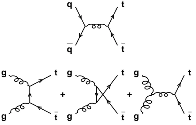
The top quark is pair-produced in pp collisions through quark-antiquark annihilation and gluon-gluon fusion. The Feynman diagrams of the leading order (LO) sub-processes are shown in Fig. 1. At Tevatron energies, the q ¯q → t¯t process dominates, contributing 85% of the cross section. The gg → t¯t process contributes the remaining 15%. q q t t g g t t g g t t g g t t + +

FIG. 1: Leading order Feynman diagrams for the production of tt pairs at the Tevatron.

The total top quark pair production cross section for a hard scattering process initiated by a pp collision at the center of mass energy √s is a function of the top quark mass mtand can be expressed as

σpp→tt+X(s, mt) = X i,j=q,q,g Z dxidxjfi(xi, µ2) (1) ×fj(xj, µ2)ˆσij→tt(ρ, m2t, αs(µ2), µ2).

The summation indices i and j run over the light quarks and gluons, xi and xj are the momentum

frac-tions of the partons involved in the pp collision, and fi(xi, µ2) and fj(xj, µ2) are the parton distribution

func-tions (PDFs) for the proton and the antiproton, respec-tively. ˆσij→tt_{(ρ, m}2

t, αs(µ2), µ2) is the total short

dis-tance cross section at ˆs ≡ xi· xj· s, and is computable as

a perturbative expansion in αs. The renormalization and

factorization scales are chosen to be the same parameter µ, with dimensions of energy, and ρ ≡ 4m2t

ˆ

s . The

the-oretical uncertainties on the tt cross section arise from the choice of µ scale, PDFs, and αs. For the most

re-cent calculations of the top quark pair production cross section, the parton-level cross sections include the full NLO matrix elements [3], and the resummation of lead-ing (LL) [4] and next-to-leadlead-ing (NLL) soft logarithms [5] appearing at all orders of perturbation theory. For a top quark mass of 175 GeV, the predicted SM tt produc-tion cross secproduc-tion is 6.7+0.7_−0.9 pb−1 _{[6]. Deviations of the}

measured cross section from the theoretical prediction could indicate effects beyond QCD perturbation theory. Explanations might include substantial non-perturbative effects, new production mechanisms, or additional top quark decay modes beyond the SM. Previous measure-ments [7, 8, 9, 10] show good agreement with the theo-retical expectation.

Within the SM, the top quark decays via the weak in-teraction to a W boson and a b quark, with a branching fraction Br(t → W b) > 0.998 [11]. The tt pair decay channels are classified as follows: the dilepton channel, where both W bosons decay leptonically into an electron or a muon (ee, µµ, eµ); the l+jets channel, where one of the W bosons decays leptonically and the other hadron-ically (e+jets, µ+jets); and the all-jets channel, where both W bosons decay hadronically. A fraction of the τ leptons decays leptonically to an electron or a muon, and two neutrinos. These events have the same signature as events in which the W boson decays directly to an elec-tron or a muon and are treated as part of the signal in the l+jets channel. In addition, dilepton events in which one of the leptons is not identified are also treated as part of the signal in the l+jets channel. Two b quarks are present in the final state of a tt event which distin-guishes it from most of the background processes. As a consequence, identifying the bottom flavor of the corre-sponding jet can be used as a selection criteria to isolate the tt signal.

This article presents a new measurement [12] of the tt production cross section in the l+jets channel. The events contain one charged lepton (e or µ) from a leptonic W boson decay with high transverse momentum, miss-ing transverse energy (6ET) from the neutrino emitted in

the W boson decay, two b jets from the hadronization of the b quarks, and two non-b jets (u, d, s, or c) from the hadronic W decay; additional jets are possible due to initial (ISR) and final state radiation (FSR). b jets in the event are identified by explicitly reconstructing secondary vertices; the addition of the silicon microstrip tracker to the upgraded detector in Run II made this technique feasible for the first time at D0.

This paper is organized as follows: the Run II D0 de-tector is described in Section II with special emphasis on those aspects that are relevant to this analysis. The trig-ger and event reconstruction/particle identification tech-niques used to select events that contain an electron or muon and jets are discussed in Sec. III and IV. The methods used to simulate tt and background events are explained in Sec. V. A data-based method that is used to estimate the contribution from instrumental and physics backgrounds to the l+jets sample is presented in Sec. VI. The methods used to estimate the efficiency and fake rate of the b tagging algorithm are explained in Sec. VII. The means for estimating all contributions to the l+jets sam-ple after tagging are detailed in Sec. VIII. Finally, the description of the method used to extract the cross sec-tion is presented in Sec. IX. The simulasec-tion of W boson events produced in association with jets is detailed in Ap-pendix A, and the handling of the statistical uncertainty on the cross section extraction procedure is explained in Appendix B.

II. THE D0 DETECTOR

The D0 detector [13] is a multi-purpose apparatus de-signed to study pp collisions at high energies. It consists of three major subsystems. At the core of the detector, a magnetized tracking system precisely records the tra-jectories of charged particles and measures their trans-verse momenta. A hermetic, finely-grained uranium and liquid argon calorimeter measures the energies of electro-magnetic and hadronic showers. A muon spectrometer measures the momenta of muons.

A. Coordinate System

The Cartesian coordinate system used for the D0 de-tector is right-handed with the z axis parallel to the di-rection of the protons, the y axis vertical, and the x axis pointing out from the center of the accelerator ring. A particular reformulation of the polar angle θ is given by the pseudorapidity defined as η ≡ − ln(tan θ/2). In addi-tion, the momentum vector projected onto a plane per-pendicular to the beam axis (transverse momentum) is defined as pT = p · sinθ. Depending on the choice of the

origin of the coordinate system, the coordinates are re-ferred to as physics coordinates (φ, η) when the origin is the reconstructed vertex of the interaction, or as detector

coordinates (φdet, ηdet) when the origin is chosen to be

the center of the D0 detector.

B. Luminosity Monitor

The Tevatron luminosity at the D0 interaction region is measured from the rate of inelastic pp collisions ob-served by the luminosity monitor (LM). The LM consists of two arrays of twenty-four plastic scintillator counters with photomultiplier readout. The arrays are located in front of the forward calorimeters at z = ±140 cm and occupy the region between the beam pipe and the for-ward preshower detector. The counters are 15 cm long and cover the pseudorapidity range 2.7 < |ηdet| < 4.4.

The uncertainty on the luminosity is currently estimated to be 6.1% [14].

C. The Central Tracking System

The purpose of the central tracking system [15] is to measure the momenta, directions, and signs of the elec-tric charges for charged particles produced in a collision. The silicon microstrip tracker (SMT) is located closest to the beam pipe and allows for an accurate determination of impact parameters and identification of secondary ver-tices. The length of the interaction region (σ ≈ 25 cm) led to the design of barrel modules interspersed with disks, and assemblies of disks in the forward and back-ward regions. The barrel detectors measure primarily the r-φ coordinate, and the disk detectors measure r-z as well as r-φ. The detector has six barrels in the central region; each barrel has four silicon readout layers, each composed of two staggered and overlapping sub-layers. Each barrel is capped at high |z| with a disk of twelve double-sided wedge detectors, called an F-disk. In the far forward and backward regions, a unit consisting of three F-disks and two large-diameter H-disks provides tracking at high |ηdet| < 3.0. Ionized charge is collected by p or n

type silicon strips of pitch between 50 and 150 µm that are used to measure the position of the hits. The axial hit resolution is of the order of 10 µm, the z hit resolution is 35 µm for 90◦_{stereo and 450 µm for 2}◦_{stereo detector}

modules.

Surrounding the SMT is the central fiber tracker (CFT), which consists of 835 µm diameter scintillating fibers mounted on eight concentric support cylinders and occupies the radial space from 20 to 52 cm from the center of the beam pipe. The two innermost cylinders are 1.66 m long, and the outer six cylinders are 2.52 m long. Each cylinder supports one doublet layer of fibers oriented along the beam direction and a second doublet layer at a stereo angle of alternating +3◦ _{and −3}◦_{. In}

each doublet the two layers of fibers are offset by half a fiber width to provide improved coverage. The CFT has a cluster resolution of about 100 µm per doublet layer.

The momenta of charged particles are determined from their curvature in the 2 T magnetic field provided by a 2.7 m long superconducting solenoid magnet [16]. The superconducting solenoid, a two layer coil with mean ra-dius 60 cm, has a stored energy of 5 MJ and operates at 10 K. Inside the tracking volume, the magnetic field along the trajectory of any particle reaching the solenoid is uniform within 0.5%. The uniformity is achieved in the absence of a field-shaping iron return yoke by using two grades of conductor. The superconducting solenoid coil plus cryostat wall has a thickness of about 0.9 radiation lengths in the central region of the detector.

Hits from both tracking detectors are combined to reconstruct tracks. The measured momentum resolu-tion of the tracker can be parameterized as σ(1/pT)

1/pT =

q

(0.003pT)2

L4 +

0.0262

L sin θ, with the first term accounting for

the measurement uncertainty of the individual hits in the tracker, and the second term for the multiple scat-tering. In the expression above, pT is the particle’s

transverse momentum (in GeV), and L is the normalized track bending lever arm. L is equal to 1 for tracks with |η| < 1.62 and equal to tan θ

tan θ′ otherwise. θ′represents the

angle at which the track exits the tracker.

D. The Calorimeter System

The uranium/liquid-argon sampling calorimeters con-stitute the primary system used to identify electrons, photons, and jets. The system is subdivided into the central calorimeter (CC) covering roughly |ηdet| < 1

and two end calorimeters (EC) extending the coverage to |ηdet| ≈ 4. Each calorimeter contains an

electromag-netic (EM) section closest to the interaction region, fol-lowed by fine and coarse hadronic sections with modules that increase in size with the distance from the inter-action region. Each of the three calorimeters is located within a cryostat that maintains the temperature at ap-proximately 80 K. The EM sections use thin 3 or 4 mm plates made from nearly pure depleted uranium. The fine hadronic sections are made from 6 mm thick uranium-niobium alloy. The coarse hadronic modules contain rela-tively thick 46.5 mm plates of copper in the CC and stain-less steel in the EC. The intercryostat region, between the CC and the EC calorimeters, contains additional layers of sampling, the scintillator-based intercryostat detector, to improve the energy resolution. The CC and EC con-tain approximately seven and nine interaction lengths of material respectively, ensuring containment of nearly all particles except high pT muons and neutrinos.

The preshower detectors are designed to improve the identification of electrons and photons and to correct for their energy losses in the solenoid during offline event reconstruction. The central preshower detector (CPS) is located in the 5 cm gap between the solenoid and the CC, covering the region |ηdet| < 1.3. The two forward

preshower detectors (FPSs) are attached to the faces of

the ECs and cover the region 1.5 < |ηdet| < 2.5. The

relative momentum resolution for the calorimeter system is measured in data and found to be σ(pT)/pT ≈ 13% for

50 GeV jets in the CC and σ(pT)/pT ≈ 12% for 50 GeV

jets in the ECs. The energy resolution for electrons in the CC is σ(E)/E ≈ 15%√E ⊕ 4%.

E. The Muon System

The muon system [17] is the outermost part of the D0 detector. It surrounds the calorimeters and serves to identify and trigger on muons and to provide crude measurements of momentum and charge. It consists of a system of proportional drift tubes (PDTs) that cover the region of |ηdet| < 1.0 and mini drift tubes (MDTs) that

extend coverage to |ηdet| ≈ 2.0. Scintillation counters are

used for triggering and for cosmic and beam-halo muon rejection. Toroidal magnets and special shielding com-plete the muon system. Each subsystem has three layers, with the innermost layer located between the calorimeter and the iron of the toroid magnet. The two remaining layers are located outside the iron. In the region directly below the CC, only partial coverage by muon detectors is possible to accomodate the support structure for the detector and the readout electronics. The average energy loss of a muon is 1.6 GeV in the calorimeter and 1.7 GeV in the iron; the momentum measurement is corrected for this energy loss. The average momentum resolution for tracks that are matched to the muon and include infor-mation from the SMT and the CFT is measured to be σ(pT) = 0.02 ⊕ 0.002pT (with pT in GeV).

III. TRIGGERS

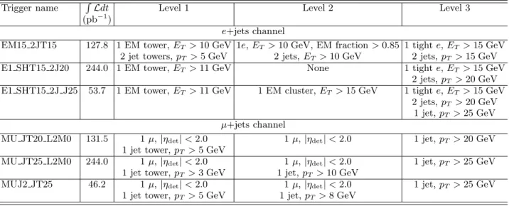
The trigger system is a three-tiered pipelined system. The first stage (Level 1) is a hardware trigger that con-sists of a framework built of field programmable gate arrays (FPGAs) which take inputs from the luminosity monitor, calorimeter, central fiber tracker, and muon sys-tem. It makes a decision within 4.2 µs and results in a trigger accept rate of about 2 kHz. In the second stage (Level 2), hardware processors associated with specific subdetectors process information that is then used by a global processor to determine correlations among differ-ent detectors. Level 2 has an accept rate of 1 kHz at a maximum dead-time of 5% and a maximum latency of 100 µs. The third stage (Level 3) uses a computing farm to perform a limited reconstruction of the event and make a trigger decision using the full event information, further reducing the rate for data recorded to tape to 50 Hz. Throughout this analysis, the data sample was selected at the trigger level by requiring the presence of a lepton and a jet; however, the required quality criteria and thresholds differ between running periods, shown in chronological order in Table I.

Trigger name R Ldt Level 1 Level 2 Level 3 (pb−1₎

e+jets channel

EM15 2JT15 127.8 1 EM tower, ET > 10 GeV 1e, ET > 10 GeV, EM fraction > 0.85 1 tight e, ET> 15 GeV

2 jet towers, pT> 5 GeV 2 jets, ET> 10 GeV 2 jets, pT> 15 GeV

E1 SHT15 2J20 244.0 1 EM tower, ET > 11 GeV None 1 tight e, ET> 15 GeV

2 jets, pT> 20 GeV

E1 SHT15 2J J25 53.7 1 EM tower, ET > 11 GeV 1 EM cluster, ET > 15 GeV 1 tight e, ET> 15 GeV

2 jets, pT> 20 GeV

1 jet, pT> 25 GeV

µ+jets channel

MU JT20 L2M0 131.5 1 µ, |ηdet| < 2.0 1 µ, |ηdet| < 2.0 1 jet, pT> 20 GeV

1 jet tower, pT> 5 GeV

MU JT25 L2M0 244.0 1 µ, |ηdet| < 2.0 1 µ, |ηdet| < 2.0 1 jet, pT> 25 GeV

1 jet tower, pT> 3 GeV 1 jet, pT > 10 GeV

MUJ2 JT25 46.2 1 µ, |ηdet| < 2.0 1 µ, |ηdet| < 2.0 1 jet, pT> 25 GeV

1 jet tower, pT> 5 GeV 1 jet, pT> 8 GeV

TABLE I: Summary of the trigger definitions used for data collection. The trigger names indicate the different running periods that correspond to the same trigger conditions. The integrated luminosity corresponding to each running period is shown in the second column.

used to measure the probability of a single object sat-isfying a particular trigger requirement. Offline recon-structed objects are then identified in the events, and the efficiency is given by the fraction of these objects that satisfy the trigger condition under study. Single ob-ject efficiencies are in general parameterized as functions of the kinematic variables pT, η, and φ of the offline

re-constructed objects. The total probability for an event to satisfy a set of trigger requirements is obtained assuming that the probability for a single object to satisfy a spe-cific trigger condition is independent of the presence of other objects in the event.

The efficiency for a tt event to satisfy a particular trig-ger condition is measured by folding into Monte Carlo (MC) simulated events the per-electron, per-muon, and per-jet efficiencies for individual trigger conditions at Level 1, Level 2, and Level 3. The total event proba-bility P (L1, L2, L3) is then calculated as the product of the probabilities for the event to satisfy the trigger con-ditions at each triggering level:

P (L1, L2, L3) = P (L1) · P (L2|L1) · P (L3|L1, L2),

where P (L2|L1) and P (L3|L1, L2) represent the condi-tional probabilities for an event to satisfy a set of criteria given it has already passed the offline selection and the requirements imposed at the previous triggering level(s). The overall trigger efficiency for tt events correspond-ing to the data samples used in this analysis is calculated as the luminosity-weighted average of the event probabil-ity associated with the trigger requirements correspond-ing to each runncorrespond-ing period. The systematic uncertainty on the trigger efficiency is obtained by varying the trigger efficiency parameterizations by ±1σ.

IV. EVENT RECONSTRUCTION AND

SELECTION

A collection of software algorithms performs the offline reconstruction of each event, identifying physics objects (tracks, primary and secondary vertices, electrons, pho-tons, muons, jets and their flavor, and 6ET) and

determin-ing their kinematic properties. Various data samples are then selected based on the objects present in the event. The following sections describe the offline event recon-struction and sample selection used for this analysis.

A. Tracks and Primary Vertex

Charged particles leave hits in the central tracking sys-tem from which tracks are reconstructed. The track re-construction and primary vertex identification are done in several steps: adjacent SMT or CFT channels above a certain threshold are grouped into clusters; sets of clus-ters which lie along the path of a particle are identified; a road-based algorithm is used for track finding, followed by a Kalman filter [18] algorithm for track fitting. The vertex search procedure [19] consists of three steps: track clustering, track selection, and vertex finding and fitting. First, tracks are clustered along the z coordinate, starting from the track with the highest pT and adding tracks to

the z-cluster if the distance between the position along z of the point of closest approach of the track to the z-cluster and the average z-cluster position is less than 2 cm. The value of this cut is optimized to effectively cluster tracks belonging to the same interaction, while being able to resolve multiple interactions. Next, qual-ity cuts are applied to the reconstructed tracks in every z-cluster requiring that they have at least 2 SMT hits, pT ≥ 0.5 GeV, and that they are within three standard

deviations of the nominal transverse interaction position. Finally, for every z-cluster, a tear-down vertex search al-gorithm fits all selected tracks to a common vertex, ex-cluding individual tracks from the fit until the total ver-tex χ2_{per degree of freedom is less than ten. The result}

of the fit is a list of reconstructed vertices that contains the hard scatter primary vertex (PV) and any additional vertices produced in minimum bias interactions. The PV is identified from this list based on the pT spectrum of the

particles associated with each interaction. The log₁₀pT

distribution of tracks from minimum bias processes is used to define a probability for a track to come from a minimum bias vertex. The probability for a vertex to originate from a minimum bias interaction is obtained from the probabilities for each track and is independent of the number of tracks used in the calculation. The ver-tex with the lowest minimum bias probability is chosen as the PV.

To ensure a high reconstruction quality for the PV, the following additional requirements have to be satis-fied: the position along z of the PV (PVz) has to be

within 60 cm of the center of the detector and at least three tracks have to be fitted to form the PV. The ef-ficiency of the PV reconstruction is about 100% in the central |z| region, but drops quickly outside the SMT fiducial volume (|z| < 36 cm for the barrel) due to the requirement of two SMT hits per track forming the PV. The two tracking detectors locate the PV with a resolu-tion of about 35 µm along the beamline [13].

B. Electrons

Electrons are reconstructed [9] using information from the calorimeter and the central tracker. A simple cone algorithm of radius ∆R = 0.2, where ∆R = (∆φ2 ₊

∆η2₎1/2_{, clusters calorimeter cells around seeds with}

ET >1.5 GeV.

An extra-loose electron is defined as an EM cluster that is almost entirely contained within the EM layers of the calorimeter, is isolated from hadronic energy deposi-tions, and has longitudinal and transverse shapes consis-tent with the expectations from simulated electrons. An extra-loose electron that has been spatially matched to a central track is called a loose electron. A loose elec-tron is considered tight if it passes a 7-variable likelihood test designed to distinguish between electrons and back-ground. The likelihood takes into account both tracking and calorimeter information, and provides more power-ful discrimination than individual cuts on the same vari-ables.

C. Muons

Muons are reconstructed using information from the muon detector and the central tracker. Local muon tracks are required to have hits in all three layers of the

muon system, be consistent with production in the pri-mary collision based on timing information from associ-ated scintillator hits, and be locassoci-ated within |ηdet| < 2.0.

Tracks are then extended to the point of closest approach to the beamline, and a global fit is performed consider-ing all central tracks within one radian in azimuthal and polar angles. The central track with the highest χ2

prob-ability is assigned to the muon candidate. The muon pT,

η, and φ are taken from the matching central track. To reject muons from semileptonic heavy flavor decays, the distance of closest approach of the muon track to the PV is required to be < 3σ; in addition, the muon is required to be isolated. Two different isolation criteria are used in this analysis [9]: the loose muon isolation criterion requires that the muon be separated from jets, ∆R(µ, jet) > 0.5. The tight muon isolation criterion requires, in addition, that the muon not be surrounded by activity in either the calorimeter or the tracker.

D. Jets

Jets are reconstructed in the calorimeter using the im-proved legacy cone algorithm [20] with radius 0.5 and a seed threshold of 0.5 GeV. A cell-selection algorithm keeps cells with energies at least 4σ above the average electronic noise and any adjacent cell with energy at least 2σ above the average electronic noise (T42 algo-rithm). Reconstructed jets are required to be confirmed by the independent trigger readout, have a minimum pT

of 8 GeV, and be separated from extra-loose electrons by ∆R(jet, e) > 0.5.

The pT of each reconstructed jet is corrected for

calorimeter showering effects, overlaps due to multiple interactions and event pileup, calorimeter noise, and the energy response of the calorimeter. The calorimeter re-sponse is measured from the pT imbalance in photon +

jet events. Jets containing a muon (∆R(µ, jet) < 0.5) are considered to originate from a semileptonic b quark decay and are corrected for the momentum carried by the muon and the neutrino. For this correction, it is assumed that the neutrino carries the same momentum as the muon. The relative uncertainty on the jet energy calibration is ≈ 7% for jets with 20 < pT < 250 GeV.

E. Missing ET

The presence of a neutrino in an event is inferred from the imbalance of the energy in the transverse plane. This imbalance is reconstructed from the vector sum of the transverse energies of the cells selected by the T42 algo-rithm; cells of the coarse hadronic calorimeter are only included if they are clustered within jets. The vector op-posite to this total visible energy vector is denoted the missing energy vector and its modulus is the raw miss-ing transverse energy (6ET raw). The calorimeter missing

sub-tracting the electromagnetic and jet response corrections applied to reconstructed objects in the event. Finally, the transverse momenta of all muons present in the event are subtracted (after correcting for the expected energy de-position of the muon in the calorimeter) to obtain the 6ET

of the event.

F. b Jets

The secondary vertex tagging algorithm (SVT) identi-fies jets arising from bottom quark hadronization (b jets) by explicitly reconstructing the decay vertex of long-lived b-flavored hadrons within the jet. The algorithm is tuned to identify b jets with high efficiency, referred to as the b tagging efficiency, while keeping low the probability of tagging a light jet (from a u, d, or s quark or a gluon), referred to as the mistag rate. The efficiency to tag a jet arising from charm quark hadronization (c jets) is re-ferred to as the c tagging efficiency. The algorithm pro-ceeds in three main steps: identification of the PV, recon-struction of displaced secondary vertices (SVs), and the association of SVs with calorimeter jets. The first step is described in Sec. IV A, the last two steps are described below.

On average, two-thirds of the particles within a jet are electrically charged and are therefore detected as tracks in the central tracking system. For each track, the distance of closest approach between the track and the beamline is referred to as dca. The z-position of the projection of the dca on the beamline is referred to as zdca. An algorithm has been developed [19] to cluster tracks into so-called track-jets. Following the procedure described in Sec. IV A tracks are grouped according to their zdca with respect to z = 0. Looping in decreasing order of track pT, tracks are added to this pre-cluster if

the difference between the track zdca and the pre-cluster z position is less than 2 cm. Next, each pre-cluster is associated with the vertex with the highest track mul-tiplicity within 2 cm of the center of the pre-cluster, and tracks satisfying the following criteria are selected: pT > 0.5 GeV, ≥ 1 hits in the SMT barrels or F-disks,

|dca| < 0.2 cm, and |zdca| < 0.4 cm, where dca and zdca are calculated with respect to the reconstructed vertex associated with the cluster. Finally, for each pre-cluster, a track-jet is formed by clustering the selected tracks with a simple cone algorithm of radius ∆R = 0.5 in (η, φ) space. The procedure adds individual tracks to the jet cone in decreasing order of track pT, and re-computes

the jet variables by adding the track 4-momentum. The process is repeated until no more seed tracks are left.

The secondary vertex finder is applied to every track-jet in the event with at least two tracks. As a first step, the algorithm loops over all tracks selecting only those with dca significance |dca/σ(dca)| > 3.5. Next, the algo-rithm uses a build-up method that finds two-track seed vertices by fitting all combinations of pairs of selected tracks within a track-jet. Additional tracks pointing to

the seeds are attached to the vertex if they improve the resulting vertex χ2_{/dof. The process is repeated until no}

additional tracks can be associated with seeds. This pro-cedure results in vertices that might share tracks. The vertices found are required to satisfy the following set of conditions: track multiplicity ≥ 2, vertex transverse decay length |~Lxy| = |~rSV − ~rP V| < 2.6 cm, vertex

transverse decay length significance |Lxy/σ(Lxy)| > 7.0,

χ2

vertex/degrees of freedom < 10, and |colinearity| > 0.9.

The colinearity is defined as ~Lxy · ~pTvtx/|~Lxy|| ~pTvtx|,

where ~pTvtx is computed as the vector sum of the

mo-menta of all attached tracks after the constrained fit to the secondary vertex. The sign of the transverse decay length is given by the sign of the colinearity. Secondary vertices composed of two tracks with opposite sign are required to be inconsistent with a V0 _{hypothesis. The}

hypotheses tested by the algorithm include K0

S → π+π−,

Λ0 _{→ p}+_π−_{, and photon conversions (γ → e}+_e−_).

Sec-ondary vertices are rejected if the invariant di-track mass is consistent with the tested V0 _{mass in a mass window}

defined by ±3σ of the measured V0 _{mass resolution.}

In the final step, a calorimeter jet is identified as a b jet (also called tagged) if it contains a reconstructed SV with Lxy/σ(Lxy) > 7.0 within ∆R < 0.5. Events containing

one or more tagged jets are referred to as tagged events.

G. Data Samples

The result presented in this document is based on data recorded using the D0 detector between August 2002 and March 2004. Several data samples are used at various stages of the analysis and are defined below.

The µ+jets preselected sample is based on 422 pb−1

of data and consists of events containing one tight muon with pT > 20 GeV and |ηdet| < 2.0 that is matched to

a trigger muon, 6ET > 20 GeV separated in φ from the

muon direction, and at least one jet with pT > 20 GeV

and |ηdet| < 2.5.

The e+jets preselected sample is based on 425 pb−1of data and consists of events containing one tight electron with pT > 20 GeV and |ηdet| < 1.1 that is matched to a

trigger electron, 6ET > 20 GeV separated in φ from the

electron direction, and at least one jet with pT > 20 GeV

and |ηdet| < 2.5.

For both the µ+jets and the e+jets preselected sam-ples, events containing a second high-pT isolated lepton

are rejected to ensure orthogonality with the dilepton analysis [10]. In addition, the samples are divided into four subsamples based on their jet multiplicity: 1, 2, or 3 jets, and 4 or more jets. In each case, the leading jet is required to have pT > 40 GeV.

The preselection efficiency is measured in MC tt sam-ples that properly take into account tau leptons that sub-sequently decay leptonically to an electron or a muon. The efficiency measured in MC is corrected by data-to-MC scale factors derived from control samples where the respective efficiency can be measured in both data and

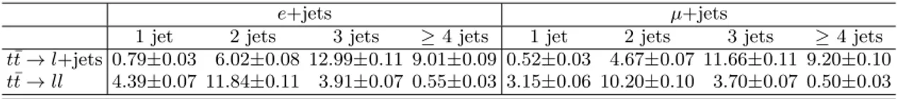
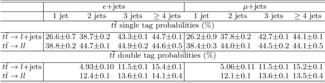
MC [9]. The quoted efficiencies include the trigger ef-ficiency for events that pass the preselection, measured by folding into the MC the per-lepton and per-jet trig-ger efficiencies measured in data, as described in Sec. III. The resulting values for the preselection efficiency for the processes t¯t → l+jets and t¯t → ll are summarized in Ta-ble II.

Systematic uncertainties in the preselection efficiencies arise from the variation of the trigger efficiencies, the data-to-MC scale factors, the jet energy scale and resolu-tion, and the jet reconstruction/identification efficiency.

In addition to the signal samples, the following samples are selected for various studies: The muon-in-jet sample contains two reconstructed jets and a non-isolated muon with ∆R(µ, jet) < 0.5. The muon-in-jet-away-jet-tagged sample is a subset of the muon-in-jet sample, where the jet opposite to the one containing the muon is tagged by SVT. The EMqcd sample contains an extra-loose electron with pT > 20 GeV, at least one reconstructed jet, and

6ET ≤ 10 GeV. The loose-minus-tight sample consists of

events that pass the e+jets preselection, except that the electron passes the loose but fails the tight selection.

V. EVENT SIMULATION

Signal and background samples are produced using the MC event simulation methods described below. In each case, generated events are processed through the geant3-based [21] D0 detector simulation and recon-structed with the same program used for collider data. Small additional corrections are applied to all recon-structed objects to improve the agreement between col-lider data and simulation. In particular, the momentum scales and resolutions for electrons and muons in the MC were tuned to reproduce the corresponding leptonic Z boson invariant mass distribution observed in data, and MC jets were smeared in energy according to a random Gaussian distribution to match the resolutions observed in data for the different regions of the detector. Over-all, good agreement is observed between reconstructed objects in data and MC.

For all MC samples, the jet flavor (b, c, or light) is de-termined by matching the direction of the reconstructed jet to the hadron flavor within the cone ∆R < 0.5 in (η, φ) space. If there is more than one hadron found within the cone, the jet is considered to be a b jet if the cone contains at least one b-flavored hadron. It is called a c jet if there is at least one c-flavored hadron in the cone and no b-flavored hadron. Light jets are required to have no b or c-flavored hadrons within ∆R < 0.5.

Production and decay of the tt signal are simulated us-ing alpgen 1.3 [22], which includes the complete 2 → n partons (2 < n < 6) Born-level matrix elements, followed by pythia 6.2 [23] to simulate the underlying event and the hadronization. The top quark mass is set to 175 GeV. evtgen [24] is used to provide the various branching fractions and lifetimes for heavy-flavor states. The

fac-torization and renormalization scales for the calculation of the tt process are set to Q = mt. MC samples are

generated separately for the dilepton and l+jets signa-tures, according to the decay of the W bosons. Leptons include electrons, muons, and taus, with taus decaying inclusively using tauola [25].

The W +jets boson background is simulated using the same MC programs; the factorization and renormaliza-tion scales are set to Q2_{= M}2

W +P (p jet

T )2. The events

are subdivided into four disjoint samples with 1, 2, or 3 jets, and 4 or more jets in the final state. Details on the generation of these samples can be found in Appendix A. Additional samples are generated for single top quark production (using comphep [26] followed by pythia), diboson production (using alpgen followed by pythia), and Z/γ∗_{→ ττ boson production (using pythia). Since}

the cross sections provided by alpgen correspond to LO calculations, correction factors are applied to scale them up to the NLO cross sections [27]. Table III summarizes the generated processes with the corresponding cross sec-tions and NLO correction factors where applicable. For Z/γ∗ _{→ ττ, the cross section is quoted at NNLO and}

corresponds to the mass range 60 < MZ < 130 GeV.

VI. COMPOSITION OF THE PRESELECTED

SAMPLES

The preselected samples are dominated by events con-taining a high pT isolated lepton originating from the

decay of a W boson accompanied by jets. These events are referred to as W -like events. The samples also in-clude contributions from QCD multijet events in which a jet is misidentified as an electron (e+jets channel), or in which a muon originating from the semileptonic decay of a heavy quark appears isolated (µ+jets channel). In addition, substantial 6ET can arise from fluctuations and

mismeasurements of the jet energies. These instrumental backgrounds are referred to as the QCD multijet back-ground, and their contribution is directly estimated from data, following the matrix method.

The matrix method relies on two data sets: a tight sample that consists of Ntevents that pass the

preselec-tion, and a loose sample that consists of Nℓ events that

pass the preselection but have the tight lepton require-ment removed, i.e., the likelihood cut for electrons and the tight isolation requirement for muons are dropped. The number of events with leptons originating from a W boson decay is denoted by Nsig_{. The number of events}

originating from QCD multijet production is denoted by NQCD_{. N}

ℓ and Ntcan be written as:

Nℓ = Nsig+ NQCD

Nt = εsigNsig+ εQCDNQCD. (2)

εsig is the efficiency for a loose lepton from a W boson

decay to pass the tight criteria; it is measured in W +jets MC events, and corrected by a data-to-MC scale factor

e+jets µ+jets

1 jet 2 jets 3 jets ≥ 4 jets 1 jet 2 jets 3 jets ≥ 4 jets

t¯t → l+jets 0.79±0.03 6.02±0.08 12.99±0.11 9.01±0.09 0.52±0.03 4.67±0.07 11.66±0.11 9.20±0.10 t¯t → ll 4.39±0.07 11.84±0.11 3.91±0.07 0.55±0.03 3.15±0.06 10.20±0.10 3.70±0.07 0.50±0.03

TABLE II: Summary of preselection efficiencies (%) for tt events. Statistical uncertainties only are quoted.

Process σ (pb) NLO correction Branching ratio

e µ tb → lνbb 0.88 – 0.1259 0.1253 tbq → lνbbj 1.98 – 0.1259 0.1253 W W → lνjj 2.04 1.31 0.3928 0.3912 W Z → lνjj 0.61 1.35 0.3928 0.3912 W Z → jjll 0.18 1.35 0.4417 0.4390 ZZ → jjll 0.16 1.28 0.4417 0.4390 Z/γ∗ → τ τ 253 – 0.3250 0.3171

TABLE III: Cross sections for background processes and the corresponding NLO correction factors, where applicable.

derived from Z → ll events. εQCD is the rate at which a

loose lepton in QCD multijet events is selected as being tight; it is measured in a low 6ET data sample which is

dominated by QCD multijet events.

The linear system in Eq. 2 can be solved for NQCD

and Nsig_{; the number of W -like events in the preselected}

samples is obtained as Ntsig = εsigNsig, and the number

of QCD multijet events as NtQCD = εQCDNQCD. The

result is summarized in Table IV. The systematic uncer-tainties on the numbers of events are obtained by varying εsig and εQCD separately by one standard deviation and

adding the results of the two variations in quadrature. As can be observed, W -like events dominate the preselected samples.

1 jet 2 jets 3 jets ≥ 4 jets e+jets Nt 6153 2217 466 119 Ntsig 5806±83 1976±50 395±23 99.8±11.6 NtQCD 347±18 241±11 71±5 19.2±2.3 µ+jets Nt 6827 2267 439 100 Ntsig 6607±85 2155±50 406±22 91.4±10.7 NQCD t 220±12 112±10 33±5 8.6±2.0

TABLE IV: Numbers of preselected events and expected con-tributions from W -like and QCD multijet events as a function of jet multiplicity. Statistical uncertainties only are quoted.

VII. SECONDARY VERTEXb TAGGING

Most of the non-tt processes found in the preselected sample do not contain heavy flavor quarks in the final state. Requiring that one or more of the jets in the event

be tagged removes approximately 95% of the background while keeping 60% of the tt events. The performance of the tagging algorithm and the methods used to de-termine the corresponding efficiencies are described in this section. The efficiencies are in general parameter-ized as functions of jet pT and |η|. For jets that contain

a muon, the jet pT is corrected by subtracting the pTs

of the muon and the neutrino. For this correction the neutrino is assumed to carry the same pT as the muon.

This procedure preserves the relationship between the pT

and the number of tracks in a jet which would otherwise be biased toward lower track multiplicities for jets that contain muons.

A. Jet Tagging Efficiencies

The probability for identifying a b jet using lifetime tagging is conveniently broken down into two compo-nents: the probability for a jet to be taggable, called taggability, and the probability for a taggable jet to be tagged by the SVT algorithm, called tagging efficiency. This breakdown of the probability decouples the tagging efficiency from issues related to detector inefficiencies, which are absorbed into the taggability.

1. Jet Taggability

A calorimeter jet is considered taggable if it is matched within ∆R < 0.5 to a jet. The tracks in the track-jet are required to have at least one hit in the SMT barrel or F-disk, effectively reducing the SMT fiducial volume to ≈ 36 cm from the center of the detector. Since this volume is smaller than the D0 luminous region (≈ 54 cm), the taggability is expected to have a strong dependence on the P Vz of the event. Moreover, the relative sign

between the P Vzand the jet η must also be considered, as

particular combinations of the position of the PV along the beam axis and the η of the jet would enhance or reduce the probability that a track-jet passes through the required region of the SMT.

Taggability is measured from a combined l+jets sam-ple passing the preselection criteria with the tight lepton requirement removed. In addition, the pT requirement on

all the jets is reduced to 15 GeV to increase the statistics of the sample. No statistically significant difference be-tween the taggability measured in this larger sample and directly in the e+jets and µ+jets preselected samples is observed. Figure 2 shows the measured taggability as a

function of P Vz and sign(P Vz× η) × |P Vz|. The

tagga-bility decreases at the edges of the SMT barrel and this effect is much more pronounced when sign(P Vz× η) > 0.

For this analysis, the taggability is parameterized as a function of jet pT and |η| in six bins of sign(P Vz× η) ×

|P Vz|: [−60, −46), [−46, −38), [−38, 0), [0,20), [20,36),

[36,60] (cm). These six regions are labeled I − VI in Fig. 2(b) and indicated by the vertical lines. They were chosen by taking into consideration the edge of the SMT fiducial region, the amount of data available for the fits, and the flatness of the taggability in each region.

(cm) Z PV -50 0 50 Taggability 0 0.2 0.4 0.6 0.8 1 (a) | (cm) Z ) x |PV jet η x Z sign(PV -50 0 50 Taggability 0 0.2 0.4 0.6 0.8 1 I II III IV V VI (b)

FIG. 2: Taggability vs. (a) P Vzand (b) sign(P Vz×η)×|P Vz|

as measured in data. The dashed lines correspond to the boundaries between regions defined in the text.

A two-dimensional parameterization of the taggability vs. jet pT and |η| is derived by assuming that the

de-pendence is factorizable, so that ε(pT, η) = Cε(pT)ε(η).

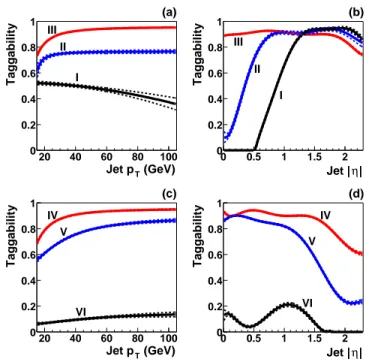
The normalization factor C is such that the total number of observed taggable jets equals the number of predicted taggable jets, calculated as the sum over all reconstructed jets weighted by their corresponding ε(pT, η). Figure 3

shows ε(pT) and ε(η) for the six regions defined above.

The assumption that the taggability can be factorized in terms of jet pT and η is verified through a

valida-tion test [28] that compares the numbers of predicted and observed taggable jets as functions of jet pT, η, P Vz,

and number of jets. For this study, the combined l+jets taggability parameterization is applied separately to the e+jets and µ+jets preselected samples as a weight for each jet. Statistical uncertainties of the fits used to de-rive the parameterizations are assigned as errors to the taggability. Good agreement between predicted and ob-served distributions is obob-served for all variables.

2. Jet Flavor Dependence of Taggability

The taggability measured in data is dominated by the predominant light quark jet contribution to the low jet multiplicity bins. The ratios of b to light and c to light taggabilities as functions of jet pT and η are measured

in a QCD multijet MC sample and shown in Fig. 4. The largest difference in taggability, approximately 5%, is ob-served between b and light quark jets in the low pT region,

(GeV) T Jet p 20 40 60 80 100 Taggability 0 0.2 0.4 0.6 0.8 1 III II I (a) | η Jet | 0 0.5 1 1.5 2 Taggability 0 0.2 0.4 0.6 0.8 1 III II I (b) (GeV) T Jet p 20 40 60 80 100 Taggability 0 0.2 0.4 0.6 0.8 1 IV V VI (c) | η Jet | 0 0.5 1 1.5 2 Taggability 0 0.2 0.4 0.6 0.8 1 IV V VI (d)

FIG. 3: Taggability vs. jet pTand |η| for P Vz×η < 0 [(a) and

(b) respectively] and P Vz× η > 0 [(c) and (d) respectively].

The central value is shown with a solid line, and the ±1σ sta-tistical uncertainty is shown as dotted lines. The labels I−VI correspond to the regions of sign(P Vz× η) × |P Vz| defined in

Fig. 2.

corresponding to jets with low track multiplicity. The fits to the ratios are used as flavor dependent correction fac-tors to the taggability.

The systematic uncertainty on the flavor dependence of the taggability is estimated by substituting the parame-terization for b and c quark jets with the one determined from W b¯b and W c¯c MC, respectively. The default b-flavor (c-b-flavor) parameterization is retained for the cen-tral value and the observed difference between that one and the W b¯b (W c¯c) parameterization is taken as the sys-tematic uncertainty.

In comparison with light quark jets, hadronic tau lep-ton decays have a lower average track multiplicity and are therefore expected to have lower taggability. Fig-ure 5 shows the ratio of τ to light quark jet taggability as functions of jet pT and η as measured in Z/γ∗ → ττ

and Z/γ∗ _{→ q¯q MC samples. The fit to the ratio is}

used as a flavor dependent correction factor to the tag-gability of hadronic tau decays in the estimation of the Z/γ∗_{→ ττ background.}

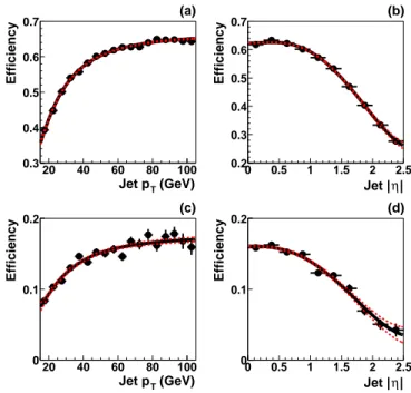
B. Tagging Efficiency

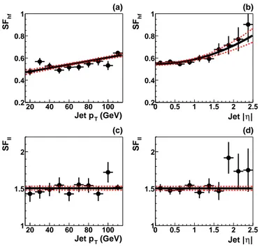
The b and c quark jet tagging efficiencies are measured in a tt MC sample and calibrated to data using a data-to-MC scale factor derived from a sample dominated by semileptonic b¯b decays. The efficiency of tagging a light

(GeV) T Jet p 20 40 60 80 100 Ratio of taggabilities_0.95 1 1.05 (a) | η Jet | 0 0.5 1 1.5 2 2.5 Ratio of taggabilities 0.95 1 1.05 (b)

FIG. 4: Ratio of the b to light (full circles) and c to light (open squares) quark jet taggability, measured in a QCD MC sample as functions of (a) jet pTand (b) jet |η|. The resulting

fits used in the analysis are also shown.

(GeV) T Jet p 20 40 60 80 100 Ratio of taggabilities 0.5 0.6 0.7 (a) | η Jet | 0 0.5 1 1.5 2 2.5 Ratio of taggabilities 0.5 0.6 0.7 (b)

FIG. 5: Ratio of the hadronic τ to light quark jet taggability, measured in Z/γ∗

→ τ τ and Z/γ∗

→ q¯q MC samples as functions of jet pT (a) and jet |η| (b). The resulting fits used

in the analysis are also shown.

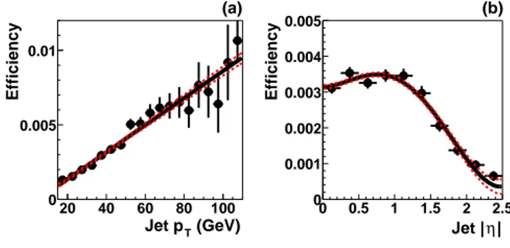
quark jet is measured in a data sample dominated by light quark jets and corrected for contamination of heavy flavor jets and long-lived particles (K0

S, Λ0). The

proce-dures followed to determine each of the tagging efficien-cies and their corresponding uncertainties are summa-rized below.

1. Semileptonic b Tagging Efficiency

The tagging efficiency for b quarks that decay semilep-tonically to muons is referred to as the semileptonic b tagging efficiency. It is measured in data using a system of eight equations (System8 Method) constructed from the total number of events in two samples with different b jet content, before and after tagging with two b tagging algorithms. The two data samples used are the muon-in-jet (n) and the muon-in-muon-in-jet-away-muon-in-jet-tagged sample (p) (see Sec. IV G for the definition of these samples). The two b tagging algorithms are SVT and the soft lepton tag-ger (SLT). The SLT algorithm requires the presence of a muon with ∆R(µ, jet) < 0.5 and prel

T > 0.7 GeV within

the jet, where prel

T refers to the muon momentum

trans-verse to the momentum of the jet-muon system. The jets are divided in two categories: b jets, and c+light (cl) jets, and the following system of eight equations is written:

n = nb+ ncl p = pb+ pcl nSVT = εSVTb nb+ εSVTcl ncl pSVT = β εSVTb pb+ α εSVTcl pcl nSLT _{= ε}SLT b nb+ εSLTcl ncl pSLT = εSLTb pb+ εSLTcl pcl nSVT,SLT = κbεSVTb εSLTb nb+ κclεSVTcl εSLTcl ncl pSVT,SLT _{= κ} bβ εSVTb εSLTb pb+ κclα εSVTcl εSLTcl pcl.

The terms on the left hand side represent the total num-ber of jets in each sample before tagging (n, p) and after tagging with the SVT algorithm (nSVT_{, p}SVT_{), the SLT}

algorithm (nSLT_{, p}SLT_{), and both (n}SVT,SLT_{, p}SVT,SLT_).

The eight unknowns on the right hand side of the equa-tions consist of the number of b and c+light jets in the two samples (nb, ncl, pb, pcl), and the tagging

efficien-cies for b and c+light jets for the two tagging algorithms (εSVT

b , εSLTb , εSVTcl , εSLTcl ). The method assumes that the

efficiency for tagging a jet with both the SVT and the SLT algorithm can be calculated as the product of the individual tagging efficiencies. Four additional parame-ters are needed to solve the system of equations: κb, κcl,

α, and β. The first two parameters represent the correla-tion between the SVT and the SLT tagger for b jets (κb)

and c+light jets (κcl), respectively. They are defined as

κb= εSVT,SLT_b εSVT b εSLTb , and κcl= εSVT,SLT_cl εSVT cl εSLTcl .

β and α represent the ratio of the SVT tagging efficien-cies for b and c+light jets, respectively, corresponding to the two data samples used to solve System8. They are defined as

β = ε

SVT

b from muon-in-jet-away-jet-tagged sample

εSVT

b from muon-in-jet sample

,

and

α = ε

SVT

cl from muon-in-jet-away-jet-tagged sample

εSVT

cl from muon-in-jet sample

.

κb, κcl, and β are measured in a MC sample mixture of

Z/γ∗_{→ b¯b → µ, Z/γ}∗_{→ c¯c, Z/γ}∗_{→ q¯q, QCD multijet,}

and tt, giving κb = 0.978±0.002, κcl= 0.826±0.014, and

β = 0.999 ± 0.006. α is arbitrarily chosen to be 1.0 ± 0.8. The system of equations is solved for each pT and η

bin separately. The resulting semileptonic b tagging effi-ciency for the SVT algorithm is shown in Fig. 6.