Adaptive Sampling of Transient Environmental
Phenomena with Autonomous Mobile Platforms
by
Victoria Lynn Preston
B.S., Olin College of Engineering (2016)
Submitted to the Department of Aeronautics and Astronautics
in partial fulfillment of the requirements for the degree of
Master of Science in Aeronautics and Astronautics
at the
MASSACHUSETTS INSTITUTE OF TECHNOLOGY AND
WOODS HOLE OCEANOGRAPHIC INSTITUTION
September 2019
© 2019 Massachusetts Institute of Technology and
Woods Hole Oceanographic Institution. All rights reserved.
Author . . . . Department of Aeronautics and Astronautics
August 22, 2019 Certified by. . . . Anna Michel Associate Scientist of Applied Ocean Physics and Engineering, WHOI Thesis Supervisor Certified by. . . . Nicholas Roy Professor of Aeronautics and Astronautics, MIT Thesis Supervisor Accepted by . . . .
Sertac Karaman Associate Professor of Aeronautics and Astronautics Chair, Graduate Program Committee Accepted by . . . .
David Ralston Associate Scientist with Tenure of Applied Ocean Physics and Engineering Chair, Joint Committee on Applied Ocean Science and Engineering
Adaptive Sampling of Transient Environmental Phenomena
with Autonomous Mobile Platforms
by
Victoria Lynn Preston
Submitted to the Department of Aeronautics and Astronautics on August 22, 2019, in partial fulfillment of the
requirements for the degree of
Master of Science in Aeronautics and Astronautics
Abstract
In the environmental and earth sciences, hypotheses about transient phenomena have been universally investigated by collecting physical sample materials and performing ex situ analysis. Although the gold standard, logistical challenges limit the overall efficacy: the number of samples are limited to what can be stored and transported, human experts must be able to safely access or directly observe the target site, and time in the field and subsequently the laboratory, increases overall campaign expense. As a result, the temporal detail and spatial diversity in the samples may fail to capture insightful structure of the phenomenon of interest.
The development of in situ instrumentation allows for near real-time analysis of physical phenomenon through observational strategies (e.g., optical), and in combi-nation with unmanned mobile platforms, has considerably impacted field operations in the sciences. In practice, mobile platforms are either remotely operated or per-form guided, supervised autonomous missions specified as navigation between human-selected waypoints. Missions like these are useful for gaining insight about a particular target site, but can be sample-sparse in scientifically valuable regions, particularly in complex or transient distributions. A skilled human expert and pilot can dynamically adjust mission trajectories based on sensor information. Encoding their insight onto a vehicle to enable adaptive sampling behaviors can broadly increase the utility of mobile platforms in the sciences.
This thesis presents three field campaigns conducted with a human-piloted marine surface vehicle, the ChemYak, to study the greenhouse gases methane (CH4) and
car-bon dioxide (CO2) in estuaries, rivers, and the open ocean. These studies illustrate
the utility of mobile surface platforms for environmental research, and highlight key challenges of studying transient phenomenon. This thesis then formalizes the max-imum seek-and-sample (MSS) adaptive sampling problem, which requires a mobile vehicle to efficiently find and densely sample from the most scientifically valuable region in an a priori unknown, dynamic environment. The PLUMES algorithm — Plume Localization under Uncertainty using Maximum-ValuE information and Search — is subsequently presented, which addresses the MSS problem and overcomes
key technical challenges with planning in natural environments. Theoretical perfor-mance guarantees are derived for PLUMES, and empirical perforperfor-mance is demon-strated against canonical uniform search and state-of-the-art baselines in simulation and field trials.
Ultimately, this thesis examines the challenges of autonomous informative sam-pling in the environmental and earth sciences. In order to create useful systems that perform diverse scientific objectives in natural environments, approaches from robotics planning, field design, Bayesian optimization, machine learning, and the sci-ences must be drawn together. PLUMES captures the breadth and depth required to solve a specific objective within adaptive sampling, and this work as a whole high-lights the potential for mobile technologies to perform intelligent autonomous science in the future.
Thesis Supervisor: Anna Michel
Title: Associate Scientist of Applied Ocean Physics and Engineering, WHOI Thesis Supervisor: Nicholas Roy
Acknowledgments
Thanks first goes to my family and friends for their support and willingness to en-tertain hours of conversation about robot boats and marine methane. I especially wish to acknowledge my parents for the freedom they provided me throughout my life to explore my interests, ultimately enabling me to become the independent (and quirky) person I am today. I also sincerely thank my partner, Bill, for his enthusiasm about my work, ability to engage in thoughtful conversations about robotics, and his enduring ability to make me laugh when the going gets tough.
To my advisers, Anna Michel and Nicholas Roy, I extend sincere gratitude for their mentorship and insight throughout my work. I recognize the fortune I have to work with two incredible professionals in two unique fields, and the opportunities for field work and learning this has afforded. Additionally, working with their labs, WHOI DSL Michel Lab and MIT CSAIL RRG, has been a pleasure. Being surrounded by thoughtful and creative minds everyday is a privilege; and I’m especially thank-ful to count these individuals among my friends. I particularly thank my research collaborators Dr.Cara Manning, Dr.David Nicholson, Dr.Yogesh Girdhar, Genevieve Flaspohler, and Kevin Manganini for their insight, patience, support, and positive attitudes throughout our work together. They have taught me so much about how to be a good scientist, engineer, and communicator.
As I hit this milestone on my way towards earning a PhD, I look forward to what the future has in store. I would like to dedicate this thesis to my parents, Matthew and Elizabeth Preston, to whom I owe my intellectual curiosity, confidence, and perseverance.
Contents
1 Introduction 15
1.1 Overview of Field Standards in Environmental and Earth Sciences . . 17
1.1.1 The “Gold Standard” . . . 18
1.1.2 In situ Instrumentation and Unmanned Platforms . . . 19
1.2 Maximum Seek-And-Sample . . . 20
1.2.1 Representing Belief . . . 21
1.2.2 Heuristic Reward . . . 22
1.2.3 Decision-Making and Planning in Continuous Domains . . . . 23
1.3 Thesis Overview . . . 25
2 Technical Background and Related Works 27 2.1 Measuring and Modeling Natural Phenomena . . . 28
2.1.1 Bayesian Inference Techniques . . . 29
2.1.2 Bayesian Representations . . . 32
2.1.3 Gaussian Processes . . . 33
2.2 Environmental Sensing as a Robotics Problem . . . 35
2.2.1 Markov Decision Processes (MDPs) . . . 35
2.2.2 Partially Observable MDPs (POMDPs) . . . 36
2.3 Reward Specification . . . 38
2.3.1 Overview of Information Measures . . . 38
2.3.2 Rewards in Bayesian Optimization . . . 40
2.4 Decision-Making under Uncertainty . . . 43
2.4.2 Online Planning . . . 43
2.5 Robots in the Wild . . . 46
3 Transience in Marine Science: Greenhouse Gas Emissions 49 3.1 Studying Methane and Carbon Dioxide . . . 50
3.1.1 Carbon Dioxide . . . 51
3.1.2 Methane . . . 52
3.1.3 Impacts . . . 52
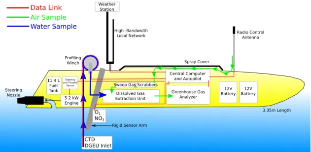
3.2 The ChemYak Mobile Platform . . . 54
3.2.1 Measurement Analysis . . . 57
3.3 Wastewater Effluent in Tidal Estuaries . . . 58
3.3.1 Overview of Field Work and Analysis . . . 59
3.3.2 Results . . . 60
3.3.3 Significance and Role of Transience . . . 66
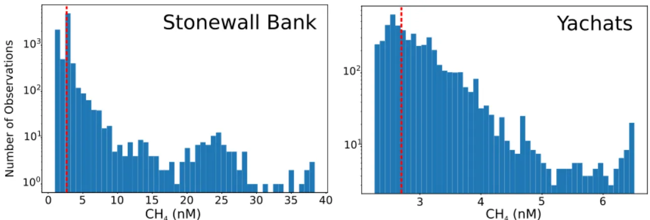
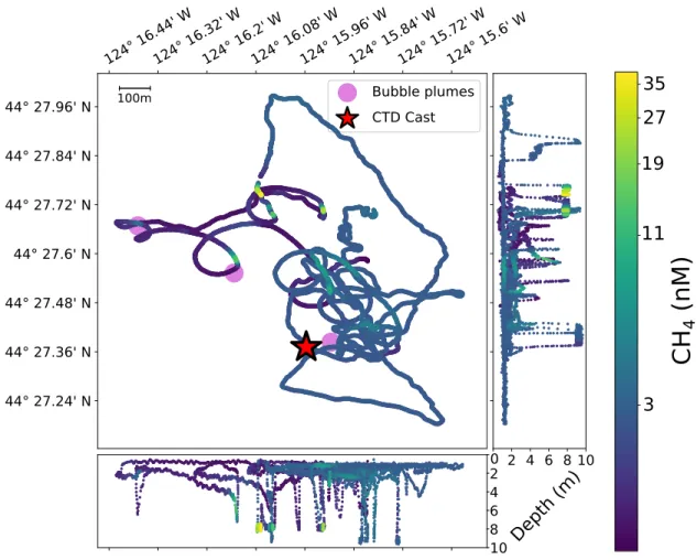
3.4 Methane Bubble Plumes in the Cascadia Margin . . . 66
3.4.1 Overview of Field Work and Analysis . . . 68
3.4.2 Results . . . 69
3.4.3 Significance and Role of Transience . . . 75
3.5 Spring Freshet River Inflow in Arctic Estuary . . . 76
3.5.1 Overview of Field Work and Analysis . . . 78
3.5.2 Results . . . 80
3.5.3 Significance and Role of Transience . . . 88
3.6 Sampling Transient Phenomenon and Motivating Adaptive Regimes . 89 4 Adaptive Sampling for Transient Phenomenon 91 4.1 Maximum Seek-and-Sample POMDP Formalism . . . 94
4.2 Representing Belief with Gaussian Processes . . . 96
4.2.1 Kernels for Natural Phenomenon . . . 96
4.3 Planning in Continuous State, Observation Spaces . . . 100
4.3.1 Analysis of Continuous Observation MCTS . . . 104
4.5 Results in Static Environments . . . 109
4.5.1 Evaluation . . . 110
4.5.2 Bounded Convex Environments . . . 111
4.5.3 Non-Convex Environments . . . 115
4.6 Results in Dynamic Environments . . . 119
4.6.1 Transience Rejection in Maximum-Value Cycling . . . 119
4.6.2 Transience Incorporation . . . 122 4.6.3 Target Tracking . . . 125 4.7 Discussion . . . 128 5 Conclusions 131 5.1 Thesis Contributions . . . 132 5.1.1 Marine Sciences . . . 132
5.1.2 Informative Path Planning and Adaptive Sampling . . . 134
5.2 Future Work . . . 135
5.2.1 Representing Scientific Phenomenon for Planning . . . 135
5.2.2 Multi-Objective Missions . . . 136
5.2.3 Longterm Monitoring . . . 136
5.2.4 Multi-Agent Systems . . . 137
List of Figures
1-1 Simple illustration of myopic and nonmyopic planning . . . 24
3-1 The ChemYak . . . 55
3-2 Wareham River: field site . . . 61
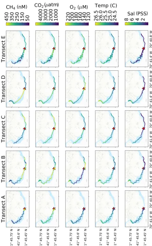
3-3 Wareham River: ChemYak transects . . . 62
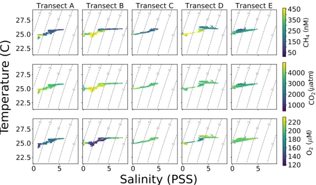
3-4 Wareham River: salinity, temperature, and gas relationships . . . 63
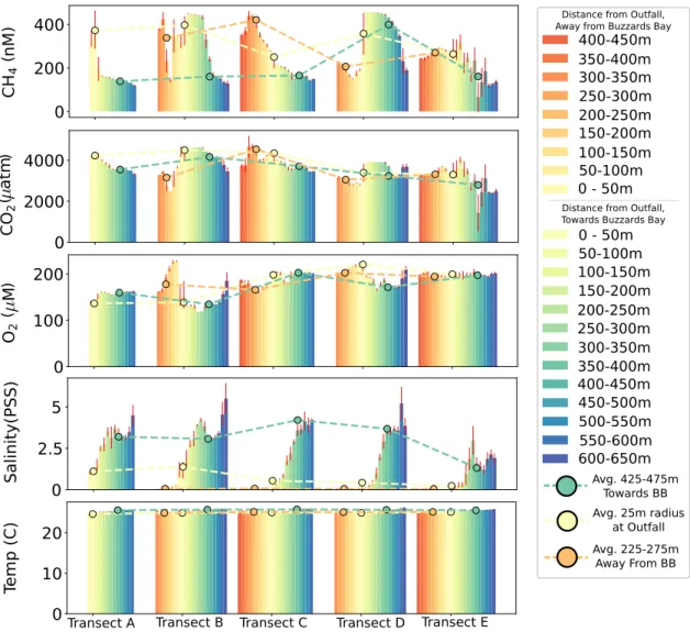
3-5 Wareham River: spatio-temporal trends . . . 65
3-6 Cascadia Margin: distribution of corrected measurements . . . 69
3-7 Cascadia Margin: Stonewall Bank ChemYak tracks . . . 71
3-8 Cascadia Margin: Yachats ChemYak tracks . . . 72
3-9 Cascadia Margin: surface methane and oxygen . . . 73
3-10 Cascadia Margin: methane depth profiles . . . 74
3-11 Cambridge Bay: reference map . . . 77
3-12 Cambridge Bay: field site and summary ChemYak tracks . . . 79
3-13 Cambridge Bay: calibration results for gas analyzer . . . 80
3-14 Cambridge Bay: depth profiles . . . 83
3-15 Cambridge Bay: spatio-temporal surface trends . . . 84
3-16 Cambridge Bay: salinity, temperature, and gas relationships . . . 85
3-17 Cambridge Bay: depth profiles binned by estuary region . . . 86
3-18 Cambridge Bay: spatio-temporal trends of the pycnocline . . . 87
4-1 GP with RBF kernels . . . 97
4-2 GP with time-varying RBF kernel . . . 98
4-4 GP with compositional Periodic-RBF kernel . . . 99 4-5 GP with dynamics model embedded in kernel . . . 100 4-6 Illustration of continuous-observation Monte-Carlo Tree Search . . . . 101 4-7 Convergence of MVI vs UCB heuristic reward . . . 109 4-8 Overview of simulation environments . . . 110 4-9 Distribution of accumulated MSS reward in static convex simulations 112 4-10 Coral head localization mission overview . . . 113 4-11 Coral head map and ASV . . . 115 4-12 Distribution of accumulated MSS reward in static non-convex simulations116 4-13 Snapshot of unknown non-convex map scenario . . . 118 4-14 Robust performance under unknown transience . . . 121 4-15 Emergent monitoring behavior with modeled transience . . . 123 4-16 Comparison of PLUMES and UCB-MCTS in modeled transience . . . 124 4-17 Trivial dynamic tracking case . . . 125 4-18 Tracking an unknown moving source . . . 127
List of Tables
4.1 Summary of metrics over static, convex simulation and field trials of PLUMES and baselines . . . 112 4.2 Summary of metrics over static, non-convex simulation and car trials
Chapter 1
Introduction
Environmental and earth sciences are an undertaking to observe and explain natural planetary processes and attributes. An interdisciplinary combination of physical, biological, chemical, geological, and information sciences, these academic fields have provided considerable insight about the places in which human life and activity are closely intertwined. In order to investigate hypotheses or characterize new discoveries, the vast majority of these disciplines require either physically realized samples (e.g., rock specimens, water samples) or direct measurements of physical attributes (e.g., temperature, gaseous concentration).
Collecting these samples or taking direct physical measurements of environmen-tal phenomena is a considerable logistical and scientific challenge. Sample collection requires that a human expert or technician can physically access the region of in-terest and interact with the phenomenon. However, in many environments, this is infeasible either due to hazards or remoteness of the region. Unmanned mobile plat-forms have increased the number of feasible study sites by explicitly going in place of human-occupied vessels. Contemporaneous development and improvement of in situ instrumentation has further improved the resolution, accuracy, and scope of ob-servations that can be gathered. Mobile “observatories” combine both unmanned vehicles and in situ sensors to gather data at various deployment scales, including: global continuous surveying (e.g., passive marine floats [1]), local monitoring (e.g., wire profilers [2]), and targeted sample retrieval (e.g., ROV [3]).
Canonically, these mobile agents navigate passively, are piloted by a human oper-ator, or autonomously traverse fixed, predetermined paths. This thesis presents three case studies in which a human-piloted marine surface vehicle was used to study the distribution of greenhouse gases in the upper water column of coastal rivers, estu-aries, and near-shore seas. These case studies illustrate the fidelity to which mobile observatories can resolve different chemical events, and highlight a major drawback with canonical methods: data sparsity in regions of interest.
Chemical expressions are transient phenomena, which display dynamic spatio-temporal behavior with spatio-temporal variation on the order of hours to days. When the robotic mission is relatively short compared to the temporal variation of the phenomenon, recovering the spatial distribution of the phenomenon dominates. In human-piloted missions, either uniform-coverage of the region is performed or reactive trajectories are executed. In both strategies, the number of samples of a target phenomenon (e.g., high concentrations of a gas species), may be relatively low if the volume of the expression is small relative to the target region, or time is spent following misleading chemical signals. When the robotic mission is on a similar timescale to the temporal variation of the phenomenon, then both spatial and temporal aspects must be recovered, further complicating these missions.
In order to densely sample interesting, dynamic phenomena in a natural environ-ment, intelligent, adaptive strategies are necessary to respond to stimulus. Adaptive sampling is an autonomy technique which uses a history of observations to inform navigation goals and mobile agent behavior to optimize a high-level scientific objec-tive. For principled sampling in spatio-temporal systems, adaptive sampling regimes can perform inference over a robot’s belief of a phenomenon based on historical ob-servations, and strategically navigate to intercept interesting events. Key questions with respect to the design and performance of an adaptive algorithm for the study of transient phenomena are:
How can scientific objectives be encoded as an adaptive sampling problem for robotic systems?
How can transient phenomena at multiple temporal scales be modeled in order to inform robotic decisions?
How should scientific value be quantified in an unknown environment?
In the face of uncountably infinite possible states of an unknown environment, what performance guarantees can an autonomous framework provide with re-spect to valuable sample collection?
This thesis presents the PLUMES algorithm, which addresses these questions and overcomes core technical challenges to allow a mobile agent to intelligently seek and densely sample from the most scientifically valuable region in an unknown natural en-vironment. The rest of this chapter is structured as follows: Section 1.1 discusses the practical challenges of sampling and collecting observations in natural environments, further motivating autonomous unmanned vehicles and introducing key vocabulary. Section 1.2 presents the motivating adaptive sampling problem of this thesis, the max-imum seek-and-sample (MSS) problem, and its core technical challenges. Section 1.3 summarizes the contributions of this thesis and previews the remaining chapters.
1.1 Overview of Field Standards in Environmental
and Earth Sciences
Within the environmental and earth sciences, sample collection and physical mea-surements are largely taken on field campaigns, which are dedicated trips to a target region. Specialized equipment to observe, measure, or capture a phenomenon of in-terest is carried on a campaign. Alternatives to field campaigns include stationary observatories, passive drifters, or remote technologies (i.e., satellites), most of which are calibrated using reference curves generated from physical samples collected and processed by human experts. Human-staffed field campaigns can target specific ge-ographic locations which may not have long-term infrastructure present, or may not be accessible by other means (e.g., satellite optical instrumentation cannot penetrate
water). Even in regions which can be observed by other means, data collected on field campaigns serve to re-calibrate instrumentation, supplement a dataset with special-ized measurements, or dynamically target a particular phenomenon.
1.1.1 The “Gold Standard”
Physically collecting (i.e., removing) singular, discrete samples of a target environ-mental phenomenon is widely considered the “gold standard” in many disciplines [4]. In order to physically collect samples of an environment, it requires that a human expert or mobile system is able to safely navigate to and from the target region and be able to appropriately store the specimen for ex situ analysis in a laboratory. In ma-rine campaigns, sample collection could involve pumping water samples from depth to a ship, or sending a Remotely Operated Vehicle (ROV) to the seafloor to retrieve sediment cores. In biological or chemical sciences, sample storage may involve us-ing a poisonus-ing chemical to terminate biological processes or addus-ing preservatives for long-term storage. Physical specimen collection and subsequent laboratory analysis provides insurance that the target phenomenon of interest is directly observed and measured. Generally, replicates are made (either by collecting multiple samples at the same location or dividing a large specimen into separate samples) and independently processed to constrain procedural error and noise.
Although the gold standard, there are notable drawbacks to relying on physical sample collection alone. The first is logistical cost: due to the monetary expense and time associated with finding, collecting, transporting, storing, and processing specimen, the total number of samples that may be realized for a region may be rel-atively few compared to the geographic extent, spatial volume, or transience of the phenomenon. This is known as “data sparsity,” and makes characterizing distribu-tions of a phenomenon in space or time challenging. In the worst case, these samples may not be representative of the true underlying distribution of a phenomenon, lead-ing to incorrect interpretations or misleadlead-ing conclusions. The second drawback is related to data analysis comparability across independent studies of similar phenom-ena. Based upon recent inter-laboratory studies in environmental chemistry, it is
unclear whether laboratories can draw consistent [5] or inconsistent [6] conclusions from equivalent samples. In general, these contradictory results inspire caution with respect to comparing published datasets or relying too closely on physical samples alone to draw conclusions.
1.1.2 In situ Instrumentation and Unmanned Platforms
Given the drawbacks of solely using collected samples, it is necessary to supplement samples with other direct observational data. In situ instrumentation records mea-surements of observations in near-real time of physical attributes that either could be confirmed by subsequent laboratory analysis, or simply may be difficult to extract in a laboratory environment at all (i.e., local temperature). Generally, this equipment is powered electrically, and the actual measurement that is observed is expressed as a voltage, which can be converted to a physical quantity by applying a calibration curve. In situ instrumentation is generally calibrated with a set of accepted labora-tory measurements, so raw observations by this equipment can be directly compared with simultaneously collected physical samples that are processed ex situ.
With the ability to take a hundred-fold more observations than traditional sample collection, surveying strategies have emerged in which a mobile platform carrying an instrument or suite of instruments is used to collect observations across a specified target region. Generally, it is desirable to perform a one-shot mission, or a single deployment of a mobile platform to collect data in a target region. Cost, time limit, and vehicle safety all play a role in this preference. Among the most common strate-gies in the environmental and earth sciences used to perform one-shot missions is uniform coverage which is also known as lawnmowing or boustrophedonic* search [7],
e.g., [8–11]. In uniform coverage, a target region is traversed by making long sweeping motions across one dimension of the region while incrementally moving in the other dimension; much like how one may methodically mow a field. Although this method enjoys simplicity in execution and guarantees with regards to spatial resolution, it
*from boustrophedon, which is a form of writing such that the lines alternate directions (right
can suffer from data sparsity in interesting regions due to its non-adaptivity.
“Autonomy” in environmental and earth sciences has generally been in the ser-vice of automating simple, predefined navigation tasks. However, with smaller and more powerful computers, improved performance of in situ sensors, and continued development in robust control and planning algorithms, intelligent autonomy is fully realizable in practice. With intelligent autonomy comes the ability to specify more complicated adaptive missions, to coordinate multi-vehicle fleets, and to create theo-retically sound guarantees about the overall quality of samples that can be collected.
1.2 Maximum Seek-And-Sample
In many environmental and earth science applications, experts want to collect scien-tifically valuable samples of a maximum (e.g., an oil spill source). This maximum could correspond with collecting the most pristine sample in an environment, the most productive source in an environment, the highest concentration area, or simi-lar attributes. The maximum seek-and-sample (MSS) problem is pervasive in many disciplines, however, natural environments are difficult to examine because they are typically unknown a priori, are continuously distributed, partially observable, and dis-play transience. This thesis presents the PLUMES adaptive sampling framework to overcome these challenges to efficiently find and sample from the global maximum of a natural environment.
Informative path planning (IPP) is a broad field which develops adaptive sampling frameworks. To encode the challenging aspects of the MSS problem, a partially-observable Markov decision process (POMDP) [12] is defined. A POMDP is a gen-eral model for decision-making under uncertainty, and is composed of a state space, observation space, action set, transition function, and reward function. In the MSS POMDP, the state and observation space are continuous functions, where the state represents the partially-observable underlying phenomenon. The action set defines the behaviors that an agent can select from, and the transition function defines how the robot’s internal model of the world, known as belief, will update according to
observations collected during an action. The reward function encodes the scientific objective of the MSS problem, giving value only to samples sufficiently close to the global maximum. Solving a POMDP exactly is generally intractable [13], and the MSS POMDP is additionally complicated by both continuous state and observation spaces, and the sparse MSS reward function. This presents the three core challenges that PLUMES addresses: compactly representing the robot’s belief of the state of the transient phenomenon, overcoming reward function sparsity, and performing online search in a belief-space over continuous functions.
1.2.1 Representing Belief
Every observation that a mobile agent collects provides partial information about the underlying state of the world. In order to plan actions, the robot must consider what it believes the complete, true state of the environment is based upon these observa-tions. A belief representation functionally stores historical observations, incorporates new observations, and can be queried while the vehicle plans what the next best ac-tion is to take. Generally, this requires that the belief representaac-tion take the form of a probability distribution over possible states, where a sample drawn from the distri-bution is one possible realization of the environmental phenomenon. This allows the robot to query the belief representation for a possible world model, evaluate actions with respect to the phenomenon distribution within that model, and consider the uncertainty associated with that model. In the MSS problem, the underlying distri-bution is a continuous function, and observations which may update the belief state are also continuous, thereby requiring that the belief representation be a probability distribution over an uncountably infinite number of possible environments.
In order to compactly represent and plan with continuous states and observa-tions, it is common in literature to discretize the state space [14, 15]. In the MSS problem, discretization over space and time is complicated by the reward function, which requires precision about the location of the global maximum. Poor choices for discretization parameters will yield poor estimates of the maximum, and subsequently poor performance for any planner. Thus, to represent the robot’s belief over
continu-ous states conditioned on a history of observations without discretization, PLUMES uses Gaussian Processes (GPs) [16]. The GP is parameterized by a mean function and a covariance kernel function. Since the environment is unknown a priori, the mean function is assumed to be uniform (e.g., uninformative). The kernel function can be used to encode both spatial and temporal relationships in an environment based upon human knowledge; for example the dispersion characteristic of a gas species in the atmosphere, or the dynamics of an oil-leaking ship. This thesis provides insight about designing kernel functions for transient phenomena, and properties of kernel functions which allow for efficient inference about natural environments.
1.2.2 Heuristic Reward
In the MSS problem, the reward function is sparse; the single non-zero reward is placed at the maximum of the world. This presents challenges for selecting useful actions, especially at the beginning of a mission when few observations are available to build a useful belief model of the target phenomenon and the location of the maximum. Planning with sparse rewards requires long-horizon information gathering and is an open problem in robotics [17]. To alleviate this difficulty, less sparse heuristic reward functions are often used in place of the true reward function, to elicit an explore-exploit behavior in the planner. In the explore phase, actions that drive down uncertainty about the world are valued, and in the exploit phase the gathered knowledge is used to target actions which more directly satisfy the scientific objective. Selecting an appropriate heuristic reward for the MSS problem requires design-ing an information-theoretic measure which elicits explore-exploit behavior, and effi-ciently converges to good estimates of the global maximum. In the field of Bayesian optimization (BO), black-box functions are typically used to optimize over an un-known function or distribution. The most commonly used heuristic reward in IPP is the Upper confidence Bound (UCB) reward [18, 19], which sums the predicted mean and variance of a proposed sample to assign a reward value. This thesis shows that for the MSS problem, UCB can lead to suboptimal behavior, and draws on work from the BO community to propose the maximum value information reward (MVI) [20]
for robotic systems. In contrast with UCB, MVI uses samples from the belief repre-sentation of the robot to distribute reward according to the possibility of finding the maximum at a particular location. As the robot examines promising regions and takes more observations, the belief representation and the location of the inferred maximum converges, and MVI places reward solely at this point, entering into the exploit phase. For the MSS problem, this reward convergence is attractive as it encourages efficient identification of and dense sample collection at the maximum.
1.2.3 Decision-Making and Planning in Continuous Domains
A planner searches over possible actions and environmental states (drawn from the belief representation) in order to find the most rewarding action or action sequence for the vehicle to take. Generally taking the form of a search tree, planners can be classified as either myopic or nonmyopic. As the name implies, myopic agents are short-sighted: they greedily take the best action based on local information. In contrast, a nonmyopic agent will choose the best action based on global information. The difference between these planners is highlighted in a demonstrative scenario shown in Fig. 1-1, in which there are two modes in the distribution of the phenomenon of interest; mode A is greater than mode B in value. The robot is given the objective to collect as many high-valued samples as possible, knows the full distribution, is initialized in a random location, and can move 1 unit in any cardinal direction. If using a myopic planner, the robot will perform gradient ascent to the nearest mode and remain there (as any other action will locally collect less reward). In this bi-modal world, if the robot is initialized near mode B, it will converge to this lower mode and fail to collect the globally optimal amount of reward, although the loca-tion of mode A is known. However, if using a nonmyopic planner, the robot may move away from mode B and towards mode A as it has the “foresight” to go to the globally optimal location, even if it requires locally suboptimal choices. Although in some environments a myopic planner may be suitable, PLUMES implements a nonmyopic planner to optimize the MVI heuristic for the attractive convergence and global planning properties.
Agent takes several locally suboptimal steps
Converges to global maximum Agent takes locally optimal steps
to quickly converge to local maxima
Ground Truth
Myopic
Nonmyopic
A
B
S S
Figure 1-1: Simple illustration of myopic and nonmyopic planning A robot tasked with collecting high-valued samples is placed in a world with two modes, A and B. Mode A is greater (more valuable) than Mode B; the global maximum is marked with a star. The robot has full knowledge of the world. When the robot is initialized close to Mode B (at the marker labeled “S”), a myopic planner (center) will take a series of locally optimal decisions and converge on Mode B. A nonmyopic planner (right) will initially take several suboptimal actions in order to converge on Mode A because it optimizes over the globally optimal action sequence.
Generally, nonmyopic search is most successful when state representations, which are nodes in the search tree, can be revisited during multiple action sequence simu-lations. By revisiting a state multiple times, the estimate of the reward that may be accumulated by reaching or traveling through that state can be better constrained. Due to the continuous observation space in the MSS problem, an uncountable set of possible belief states arises (since each observation will be unique with probability 1), creating a degenerate tree. Practically, tree degeneracy leads to inefficient deci-sions and theoretically prevents any formal guarantees regarding planner performance. Given the importance of establishing confidence for an autonomy system in the envi-ronmental and earth sciences, the key challenge to overcome is related to addressing tree degeneracy in continuous, partially-observable domains and formulating perfor-mance guarantees of the framework. This thesis extends planners for fully-observable continuous-domains [21, 22] to partially-observable domains, and demonstrates that theoretical performance guarantees are preserved.
1.3 Thesis Overview
The contributions of this thesis are:
1. Presentation of three field campaigns which analyze transient chemical phenom-ena in near-shore seas and coastal estuaries and rivers:
(a) The effect of wastewater effluent on the Wareham River, MA, USA (b) Surface expression of methane from bubble plumes in the Cascadia Margin
(c) Arctic outgassing driven by spring-time river inflow in Cambridge Bay, Nunavut, Canada
2. Formulation of the MSS problem as a POMDP
3. Presentation of the PLUMES adaptive sampling framework:
(a) Analysis of GP kernel functions to model spatio-temporal phenomena
(b) Identification, adaptation, and implementation of a BO black-box information-theoretic reward function for the MSS problem
(c) Novel analysis of a nonmyopic planner demonstrating guarantees in con-tinuous, partially-observable environments
(d) Demonstration of improved performance over baseline techniques in simu-lated and field trials
The remainder of this thesis is organized as follows: Chapter 2 presents technical background and related work on the foundations of adaptive sampling. Chapter 3 presents the three field campaigns and scientific discoveries, and discusses the role of transience in those environments. In Chapter 4, the MSS problem is formalized and the PLUMES algorithm is described in detail, including core sections on the belief representation of transient phenomena, heuristic reward function, and nonmyopic planner. Comparisons with baseline planners from literature are also presented. A summary of results and brief discussion concludes in Chapter 5.
Chapter 2
Technical Background and Related
Works
This thesis builds upon foundational work in probabilistic modeling, planning under uncertainty, and information measures in order to examine the development and use of intelligent robotic systems for environmental field campaigns. Central to this work is the concept of adaptive sampling, which is a technique that informs future behaviors of an agent or system by incorporating a history of observations. Within the fields of robotics and sensing, adaptive sampling techniques have been broadly applied in applications including:
1. Direct observation and study of environmental domains (e.g., [23–27])
2. Within localization frameworks to improve state estimates (e.g., [28–31])
3. Image processing (e.g., [32,33])
4. Distributed sensor networks (e.g., [34–36])
This chapter will primarily frame the technical discussion of core adaptive sam-pling concepts within the context of environmental samsam-pling with mobile robotic agents. Problem- and content-specific related work will be provided in each of Chap-ters 3 and 4 in technical discussions of the thesis contributions.
2.1 Measuring and Modeling Natural Phenomena
The intent of using robotic platforms in environmental and earth science campaigns is to collect “useful data” about target phenomena, which allow scientists to gain insight about an underlying process and address hypotheses. This insight is gener-ally driven by comparing data to scientific models, which encode well-characterized physical relationships between phenomenon (e.g., relationship between hypoxic zones and high methane content in deep ocean waters). Numerical models based on first principles dominate much of the sciences [37–40]. These models are incredibly expres-sive and comprehenexpres-sive. Collected data are generally used to tune free parameters or define new relationships to be incorporated into these models in order to match input conditions with realized physical observations [41].
Although the standard, numerical models are generally brittle to noisy or unex-pected measurements and do not generalize well to new datasets, largely because they rely on an assumption of determinism. This brittleness has motivated the use of statistical or probabilistic models, which can capture uncertainty in measurements and physical relationships (e.g., [42–44]). Innovation in environmental probabilistic modeling complements innovations made in robotics; kriging is perhaps the most clear example of a probabilistic model that was developed originally for characterizing geo-static phenomenon [44] and has since been widely adopted in the form of Gaussian process regression [16] in robotics and machine learning communities.
Probabilistic models are particularly attractive for robotic applications because they allow for decision-making to be informed by measures of certainty (or uncer-tainty). For example, one of the most ubiquitous probabilistic models in robotic navigation is an occupancy grid [45] which is used to model occupied, free, and un-known physical space based on observations of obstacles by an agent. The state of a grid cell is a probabilistic measure based upon the history of noisy observations collected by a robot platform and a model of the noise characteristic of the sensor. When space is uncertain, then the robot has the ability to collect more measure-ments to increase certainty, or choose alternate paths which may be believed to be
safer. However, unlike metric obstacles, environmental phenomenon are generally as-sumed to be complex, multimodal, dynamic, and stochastic. To suitably model such phenomena, this thesis primarily makes use of Gaussian processes (GPs) [16], which are a Bayesian nonparametric model from machine learning. Section 2.1.1 provides background on Bayesian inference, Section 2.1.2 describes Bayesian model representa-tions, and Section 2.1.3 specifically presents GPs and discusses work in environmental sampling which has leveraged GPs for studying phenomena.
2.1.1 Bayesian Inference Techniques
Bayesian models, as the name implies, leverage Bayes Theorem as a basis for per-forming inference over a set of unknown parameters:
𝑝(𝜃|𝑦) = 𝑝(𝑦|𝜃)𝑝(𝜃)
𝑝(𝑦) (2.1)
where Bayes Theorem states that the posterior distribution of a set of parameters 𝜃 given a dataset 𝑦 is proportional to the likelihood of the data given the set of parame-ters, and a prior distribution on the parameters. In environmental domains, the prior distribution is a way to encode knowledge about scientific principles or relationships. It has been observed that Bayesian techniques have become increasingly used in the environmental sciences [46] due to the flexibility of various Bayesian frameworks, un-certainty characterization, and robustness to variability and nondeterministic factors. A Bayesian inference problem takes the following form: let 𝒳 = {𝑋0, ..., 𝑋𝑁 −1}
be a set of 𝑁 random variables with a relationship described by joint distribution Pr(𝑋0, ...𝑋𝑁 −1). Some subset of these random variables are observed, 𝒳𝑜𝑏𝑠. Bayesian
inference allows for these observations to inform what values the unobserved, latent variables 𝒳𝑙𝑎𝑡 = 𝒳 ∖𝒳𝑜𝑏𝑠 are likely to take. A direct application of Bayes Theorem
and probability theory yields:
Pr(𝒳𝑙𝑎𝑡|𝒳𝑜𝑏𝑠) = Pr(𝒳𝑙𝑎𝑡, 𝒳𝑜𝑏𝑠) Pr(𝒳𝑜𝑏𝑠) = ∫︀ Pr(𝒳𝑙𝑎𝑡, 𝒳𝑜𝑏𝑠) 𝒳𝑙𝑎𝑡Pr(𝒳𝑙𝑎𝑡, 𝒳𝑜𝑏𝑠) (2.2) where the denominator is the marginal likelihood of the observations. In practice,
performing exact inference with Eq. 2.2 is computationally expensive to the point of being intractable: calculating the marginal likelihood is exponential in the number of latent variables. To overcome this challenge, approximation techniques are employed.
Variational Bayesian Inference One common approximate inference technique is variational Bayesian inference [47,48], which approximates a posterior distribution with a well-behaved function class, 𝑞*(𝜃) ≈ 𝑝(𝜃|𝑦). In order to identify 𝑞*(𝜃) from
class 𝑄, an optimization procedure over some distance measure 𝑓 is performed:
𝑞*(𝜃) = arg min
𝑞∈𝑄
𝑓 (𝑞(·), 𝑝(·|𝑦)) (2.3) The Kullback-Leibler (KL) divergence, KL(·||·) is a common choice for the distance metric because of good empirical performance and adaptability to fast, streaming, and distributed systems [48]. By using KL divergence, a convenient simplification for the optimization problem arises:
KL(𝑞||𝑝(·|𝑦)) = log 𝑝(𝑦) −∫︁ Θ 𝑞(𝜃) log𝑝(𝜃)𝑝(𝑦|𝜃) 𝑞(𝜃) 𝑑𝜃 (2.4) 𝑞*(𝜃) = arg max 𝑞∈𝑄 ∫︁ Θ 𝑞(𝜃) log𝑝(𝜃)𝑝(𝑦|𝜃) 𝑞(𝜃) 𝑑𝜃 (2.5)
where the ELBO (evidence lower bound) of the KL divergence is the second term in Eq. 2.4 and the optimization can primarily occur with respect the ELBO as it only contains well-defined aspects of the model.
This only leaves selecting distributions 𝑄 that are well-behaved. A common choice is to apply the mean-field approximation:
𝑄 = {𝑞 : 𝑞(𝜃) =
𝑛
∏︁
𝑖=1
𝑞𝑖(𝜃𝑖)} (2.6)
which provides that the set of distributions over the latent parameters factorizes and allows low-dimensional representations to be considered. With this family of distributions, Eq. 2.5 can be solved using simple coordinate ascent approaches [47].
[49] and automatic differentiation variational inference (ADVI) [50], have been demon-strated to improve standard variational techniques under assumptions of conjugacy or differentiable properties.
Monte Carlo Inference Methods An alternative to variational techniques to estimate the form of the true posterior 𝑝(𝜃|𝑦) are Monte Carlo (MC) methods [51]. Rather than perform an optimization over analytic functions to get a closed form for the posterior, MC methods approximate estimators (Φ) of a function 𝜑(·) with respect to the true density 𝑝(𝑦) by drawing samples from a proposal density 𝑞(𝑦). This work generally assumes that the form of 𝑝(𝑦) is known and can be evaluated to within a multiplicative constant, 𝑝(𝑦) = 𝑝*(𝑦)/𝑍, but is generally difficult to draw samples
from directly (especially in high-dimensional domains). Monte Carlo sampling instead draws samples from a more tractable, known proposal distribution 𝑞(𝑦) = 𝑞*(𝑦)/𝑍
𝑞
and evaluates those samples with respect to 𝑝*(𝑦)in order to approximate Φ. One of
the most straightforward MC samplers is importance sampling:
1. Draw 𝑥1, ...𝑥𝑁 i.i.d. samples from 𝑞(·).
2. Calculate weight 𝑤𝑖 = 𝑝*(𝑥𝑖)/𝑞*(𝑥𝑖).
3. Calculate estimate Φ = ∑︀
𝑁𝑤𝑖𝜑(𝑥𝑖)
∑︀
𝑁𝑤𝑖
Rejection sampling is another MC sampler, and leverages the intuition that some samples generated from 𝑞(𝑦) may not align well with 𝑝(𝑦). An acceptance criteria for adding a sample 𝑥𝑖 to the dataset is defined through the rule 𝑝*(𝑥𝑖) > 𝑢 where 𝑢 is a
draw from a uniform distribution with bounds [0, 𝑞*(𝑥 𝑖)].
MC methods generally require that the form of 𝑞(𝑦) lie near the form of 𝑝(𝑦). In large, complex systems, it is difficult to define a single density that captures these characteristics. Markov chain MC (MCMC) algorithms address this by drawing new samples 𝑥′ using a proposal density which relies on the state of the previous
sam-ple 𝑥(𝑡); 𝑞(𝑥′, 𝑥(𝑡)). In Metropolis-Hasting MCMC, an acceptance ratio is used to
𝑎 = 𝑝
*(𝑥′)𝑞(𝑥(𝑡); 𝑥′)
𝑝*(𝑥(𝑡))𝑞(𝑥′; 𝑥(𝑡)) (2.7)
where if 𝑎 ≥ 1 the new state 𝑥′ is accepted and 𝑥(𝑡+1) = 𝑥′; otherwise a new sample
𝑥′ is drawn from 𝑞(𝑥′, 𝑥(𝑡))and 𝑥(𝑡+1)= 𝑥(𝑡). Other MCMC samplers, like Gibbs [51],
Reversible-Jump [52], and Hamiltonian [53] use other acceptance ratios or special forms of 𝑞(𝑦) in order to improve the convergence characteristics, flexibility, and speed of Metropolis-Hastings. In all MCMC samplers, because each new state relies on a density informed by the previous state, a “burn-in” period, in which a potentially large number of samples are drawn, must be used before virtually independent samples are generated. It has been shown that for a large number of samples, the estimator generated with MC methods will converge to the true estimator of the posterior [51].
2.1.2 Bayesian Representations
In order to perform inference, a model is necessary to describe (i.e., the likelihood, prior, or other relationships between latent parameters). This section briefly describes several ways within the scope of Bayesian inference that phenomena may be modeled.
Graphical Models Probabilistic graphical models (PGMs) exploit the conditional independence structure of the latent parameters. Bayesian networks [54] are one particular form of graphical model which has enjoyed adoption in both the environ-mental sciences [55] and in robotic environenviron-mental sensing missions [15] as they allow for specific relationships between latent parameters to be encoded.
Let a Bayesian network be defined as an acyclic graph 𝒢 = (𝑉, 𝐸) where vertices 𝑉 represent random variables, and directed edges represent dependencies between two variables indexed (𝑖, 𝑗) ∈ 𝐸 where 𝑖 in this example is a parent to 𝑗. The joint probability of 𝑉 in the graph can be expressed as the product of all conditional probabilities Pr(𝑋𝑖|parents(𝑋𝑖))where the parents 𝑋𝑗 of node 𝑋𝑖 are the connected
edges (𝑗, 𝑖). In complex networks, exact inference may be intractable. Variational and MCMC techniques can be used to approximately solve a Bayesian network.
Parametric and Nonparametric Models An alternative to Bayesian networks that allow for exact inference with respect to encoded or learned relationships are parametric models. In a parametric model, a fixed number of parameters are fit to a portion of data, known as the training set. The model’s accuracy is then assessed using an unseen test set of data in a process known as cross-validation. By assessing model accuracy, different numbers or types of parameters can be designed for desired performance. Finite mixture models (e.g., [56]) are one form of parametric model.
Although typically seen as a computational advantage, in the environmental sci-ences a drawback of parametric models is that model complexity remains the same no matter the size of data available. Selecting a “good” number of parameters, or even which parameters to use a priori may be difficult for processing real observa-tions, as many phenomenon have complicated structure that may be entirely con-text dependent. In general, it would be useful if the data could directly inform the parameter-space, rather than have the parameter-space predefined. Nonparametric models were designed specifically to allow model complexity to grow with more data, and can handle a potentially infinite number of parameters.
To do this, nonparametric models capture the notion of representing probability over a collection of distribution functions. The Dirichlet process [57], the Chinese restaurant process [58], and other methods have all been proposed for generating and representing infinite-mixture models for inference. In the environmental sciences and for robotic applications within the environmental sciences, Gaussian Processes (GPs) [16] have received considerable attention [19,35,59–61].
2.1.3 Gaussian Processes
Informally, a GP is used to represent a distribution over functions. Formally, Ras-mussen and Williams define a GP in [16] as:
Definition 2.1.1. A Gaussian process is a collection of random variables, any finite number of which have a joint Gaussian distribution.
target be represented as a 𝑑-dimensional compact set X ⊂ R𝑑. The unknown
under-lying, 𝑚-dimensional continuous function is 𝑓 : X → R𝑚. For notational simplicity,
𝑚 = 1 in the following discussion. Samples of 𝑓 can be drawn in a location x with a noisy sensor: 𝑦 = 𝑓(x) + 𝜖 where 𝜖 ∼ 𝒩 (0, 𝜎2
𝑛) is normally distributed sensor noise.
A GP is fully parameterized by a mean 𝜇(x) and covariance function 𝜅(x, x′)(also
known as a kernel), which take the form:
𝜇(x) = E[𝑓 (x)] (2.8)
𝜅(x, x′) = E[(𝑓 (x) − 𝜇(x))(𝑓 (x′) − 𝜇(x′))] (2.9) so that 𝑓(x) ∼ 𝒢𝒫(𝜇(x), 𝜅(x, x′)). Given a history 𝒟
𝑡= {x𝑖, 𝑦𝑖}𝐷𝑖=0of 𝐷 observations
and observation locations at time 𝑡, the posterior belief at a new location x′
∈ X is: 𝑔𝑡(x′) | 𝒟𝑡∼ 𝒩 (𝜇𝑡(x′), 𝜎2𝑡(x ′ )),where (2.10) 𝜇𝑡(x′) = 𝜅𝑡(x′)⊤(K𝑡+ 𝜎𝑛2I) −1 y𝑡, (2.11) 𝜎𝑡2(x′) = 𝜅(x′, x′) − 𝜅𝑡(x′)⊤(K𝑡+ 𝜎𝑛2I) −1 𝜅𝑡(x′), (2.12)
where y𝑡 = [𝑦0, . . . , 𝑦𝐷−1]⊤, K𝑡 is the positive definite kernel matrix with K𝑡[𝑖, 𝑗] =
𝜅(x𝑖, x𝑗)for all x𝑖, x𝑗 ∈ 𝒟𝑡, and 𝜅𝑡(x′) = [𝜅(x0, x′), . . . , 𝜅(x𝐷−1, x′)]⊤.
In practice, 𝜇(x) is typically set to 0, and the kernel function is primarily used to encode the relationship between features in the environment. Kernel functions con-tain hyperparameters, which specify properties like smoothness, correlation strength, periodicity, and scale. Hyperparameters can be set directly through prior knowledge about a phenomenon of interest, or through online optimization techniques (e.g., [62]). The popularity of GPs for environmental modeling and robotic planning is rooted in the relative ease of training and performing inference with the representation, in addition to the simple but expressive way in which kernel hyperparameters can be utilized to enforce structure over data. In large datasets, GPs can be computationally expensive, as the training and inference time is cubic with respect to number of observations. Sparse GPs [63] can be employed to address scalability concerns.
2.2 Environmental Sensing as a Robotics Problem
Environmental sensing with a robotic platform can be considered an information-gathering mission. In such applications, the environmental model is useful for repre-senting the robot’s belief about the state of the target phenomenon with respect to a history of observations, but decision-making requires more information; a planning model is necessary. A planning model specifies the vehicle dynamics, available ac-tions, belief about the physical state of the vehicle, the precise mission objective, and a method for evaluating an action with respect to the mission objective. Information-gathering is most generally modeled as sequential decision-making in which actions are evaluated, selected, and executed at each planning iteration. Sequential decision-making processes are considered Markovian when an action selection is conditionally independent of previous actions and observations given the current belief state of the vehicle (with respect to both environmental and state model). Markov decision processes (MDPs) [64,65] are a useful model for a robotic planning problem, and are described in Sec. 2.2.1. An extension of MDPs to domains in which the state of the world is only partially observable, POMDPs [12], is presented in Sec. 2.2.2.
2.2.1 Markov Decision Processes (MDPs)
A Markov decision process (MDP) is represented as a tuple (𝒮, 𝒜, 𝑇, 𝑅, 𝛾, 𝑠0)where:
𝒮 is the set of finite or infinite (in the case of continuous functions) decision states
𝒜 is the set of finite or infinite (in the case of continuous actions) actions that are available to the vehicle, 𝒜𝑠 is the set of actions available from state 𝑠.
𝑇 : 𝒮 × 𝒜 → 𝒫(𝒮) is the transition function which represents the probability density of being in state 𝑠 ∈ 𝒮, taking action 𝑎 ∈ 𝒜, and arriving in state 𝑠′ ∈ 𝒮; 𝑇 (𝑠, 𝑎, 𝑠′) = Pr(𝒮
𝑡+1 = 𝑠′|𝒮𝑡 = 𝑠, 𝒜𝑡 = 𝑎). This allows for imperfect
𝑅 : 𝒮 × 𝒜 → R is the reward function, which represents the value of performing some action 𝑎 ∈ 𝒜 when in state 𝑠 ∈ 𝒮. Can alternatively be 𝑅 : 𝒮 ×𝒜×𝒮 → R if value is awarded by arriving into a state 𝑠′ ∈ 𝒮 from state 𝑠 ∈ 𝒮 after taking
an action 𝑎 ∈ 𝒜.
𝛾 is the discount factor which is applied in infinite-horizon missions.
𝑠𝑜 is the initial decision state.
A policy 𝜋 : 𝒮 → 𝒜 which maps decision states to actions is a solution to an MDP. An optimal policy 𝜋* describes the set of actions to take from any given state
that maximize the total (potentially discounted) reward for a ℎ-horizon mission (in which ℎ can be infinity):
𝜋* = arg max 𝜋 E [︂ inf ∑︁ 𝑡=0 𝛾𝑡𝑅(𝑠𝑡, 𝑎𝑡)|𝑠0, 𝜋 ]︂ (2.13)
The optimal policy from state 𝑠 ∈ 𝒮 can be determined using value iteration, which iteratively estimates the value of the optimal policy using the Bellman equation [65]:
𝑉𝑡+1* (𝑠) ← max 𝑎∈𝒜 [︂ ∑︁ 𝑠′∈𝒮 𝑇 (𝑠, 𝑎, 𝑠′)(𝑅(𝑠, 𝑎, 𝑠′) + 𝛾𝑉𝑡(𝑠′)) ]︂ 𝜋*(𝑠) = arg max 𝑎∈𝒜 [︂ ∑︁ 𝑠′∈𝒮 𝑇 (𝑠, 𝑎, 𝑠′)(𝑅(𝑠, 𝑎, 𝑠′) + 𝛾𝑉*(𝑠′)) ]︂ . (2.14)
For a threshold 𝜖, such that value iteration is terminated when |𝑉𝑡+1(𝑠)−𝑉𝑡(𝑠)|< 𝜖,
then max𝑠∈𝒮|𝑉𝑡+1(𝑠) − 𝑉*(𝑠)|< 2𝜖𝛾/(1 − 𝛾). Value iteration converges in polynomial
time.
2.2.2 Partially Observable MDPs (POMDPs)
At their core, MDPs assume that the state at any time is fully-observable, however, in the case of environmental sensing, a collected observation generally does not reveal the full state of the phenomenon. Thus, the underlying function 𝑓 is partially-observable.
Partially-observable Markov decision processes (POMDPs) [12] extends MDPs to par-tially observable domains, defined as the tuple (𝒮, 𝒜, 𝒵, 𝑇, 𝑂, 𝑅, 𝛾, 𝑏0)where 𝒮, 𝒜, 𝑅,
and 𝛾 are defined as in Sec. 2.2.1 with:
𝒵 is the space of all possible observations. May be finite or infinite (in the case of continuous functions).
𝑂 : 𝒮 × 𝒜 → 𝒫(𝒵) is the observation model, which represents the probability density of observation 𝑧 ∈ 𝒵 after executing action 𝑎 ∈ 𝒜 from state 𝑠 ∈ 𝒮; Pr(𝑂𝑡= 𝑧|𝒮𝑡= 𝑠, 𝒜𝑡 = 𝑎). This function can model imperfect sensing.
𝑏0 is the prior distribution over the initial state 𝒮0; 𝑏0 =Pr(𝒮0 = 𝑠)
In partially-observable domains, the state of the world is uncertain. In general, this means that the decision process is no longer Markov, as the optimal policy would no longer be dependent on the state. However, by making decisions based on the belief over states rather than making decisions based on the current best estimate of the state, the Markov property can be restored, since the belief state summarizes all the historical observation and action history relevant for policy calculation. Just as in MDPs, the Bellman equation can be used to recursively quantify the value of belief 𝑏𝑡 = 𝒫(𝑆𝑡) over horizon-ℎ under policy 𝜋 : 𝑏𝑡→ 𝑎𝑡 as:
𝑉ℎ𝜋(𝑏𝑡) = E[𝑅(𝑠𝑡, 𝜋(𝑏𝑡))] + 𝛾
∑︁
𝑧∈𝒵
𝑉ℎ−1𝜋 (𝑏𝜋(𝑏𝑡),𝑧
𝑡+1 ) Pr(𝑧 | 𝑏𝑡, 𝜋(𝑏𝑡)), (2.15)
where the expectation is taken over the current belief and 𝑏𝜋(𝑏𝑡),𝑧
𝑡+1 is the updated
belief after taking action 𝜋(𝑏𝑡) and observing 𝑧 ∈ 𝒵. The optimal policy 𝜋*ℎ over
horizon-ℎ is the maximizer of the value function over the space of possible policies Π: 𝜋ℎ* = arg max𝜋∈Π𝑉𝜋
ℎ(𝑏𝑡).
In general, Eq. 2.15 is difficult or intractable to compute in large or continuous state and observation spaces. The same holds for large or continuous-valued MDPs. Thus, approximate solvers are necessary in order to extract the optimal policy for a robotic agent to execute. Sec. 2.3 and Sec. 2.4 discuss in detail the formulation of the reward function and methods for approximately solving MDPs and POMDPs.
2.3 Reward Specification
In an MDP or POMDP formulation, the reward function serves to encode the scientific objective of a mission. For example, if the objective was to drive the vehicle to the maximizer of some distribution, then the reward function may deliver reward only to actions that directly lead to states in the proximity of the maximizer. Some objectives may be easy to encode as a heuristic reward, however in environmental domains, objectives may be less obvious to encode, e.g., “map” a phenomenon, “learn” a distribution, etc. Even with relatively straightforward objectives, like the illustrative maximizer objective above, rewards that take on a “sparse” form (i.e., the reward signal itself is only provided in very few states) are generally hard for a robot agent to optimize well [17]. In either of these cases, it is useful to consider reward functions that can quantify the value of information content of a potential observation in order to elicit explore-exploit behaviors.
Explore-exploit describes decision sequences which initially allow the agent to ex-plore the unknown state space in order to characterize the distribution and build a sophisticated belief over the domain, then exploit that knowledge in service of some objective (e.g., converging to a maximizer). Reward functions which encode this trade-off may use hyperparameters to tune the balance in the explore-exploit behav-ior, whereas other functions may naturally enforce these behaviors. Information mea-sures have been studied as suitable reward signals to encode explore-exploit behavior in several fields, including optimal experimental design, optimal sensor placement, reinforcement learning, and Bayesian optimization. This section provides a brief overview of these fields and core concepts in information measures, with particular focus on information-theoretic measures from Bayesian optimization in Sec. 2.3.2.
2.3.1 Overview of Information Measures
Information measures provide a way to assess the utility of a measurement with respect to the history of observations and ultimate objective. Several widely used information measures have been proposed in multiple fields; for details on information
measures in general, MacKay [66] provides a comprehensive overview.
Optimal Experimental Design In optimal experimental design [67], a typical experiment requires estimating a vector z ∈ R𝑑 from a set of measurements x and
observations y such that 𝑦𝑖 = 𝑥𝑇𝑖 z + 𝑤𝑖 for 𝑖 = 1...𝑁 observations, where 𝑤𝑖 is
zero-mean Gaussian noise. An estimator is then calculated for z given the experimental set-up. Commonly, the maximum likelihood estimate (MLE), ˆz, is used because it is an unbiased estimator. The estimation error between the ˆz and ˆz is 𝐸 = ˆz − z. The covariance matrix of 𝐸 is ultimately used to characterize informativeness of a measurement by inspecting how the measurements reduce overall error variance.
Several types of optimal design arise based upon different criteria for inspecting variance reduction. Some optimal design regimes used in robotics, learning, and sensing applications are listed:
𝐴-optimal: Minimizes the trace of the inverse covariance matrix, e.g., [68–70] 𝐷-optimal: Minimizes the determinant of the covariance matrix, e.g., [69–71,71] 𝐸-optimal: Maximizes the smallest eigenvalue of the covariance matrix, e.g., [70] 𝑉 -optimal: Minimize the average prediction variance, e.g., [72]
Soft Measures of Information In optimal experimental design, “hard” estimates of a target variable (i.e., explicit estimators) are used to quantify the informativeness of a measurement. In contrast, “soft” estimates use the probability distribution over a target variable. Shannon’s entropy [73] was defined with respect to four key design principles for an information measure, 𝐼(·), with respect to probability 𝑝:
1. Information measures are continuous, monotonic functions of probability; 𝐼(𝑝) 2. Information is non-negative; 𝐼(𝑝) ≥ 0
3. If an event has probability 1 (it is certain to occur), then no information is gained; 𝐼(1) = 0
4. The information gained from observing two independent events is the sum over information gained from each individual event; 𝐼(𝑝1𝑝2) = 𝐼(𝑝1) + 𝐼(𝑝2).
From these principles, entropy was defined as:
𝐻(𝑋) = −
𝑛
∑︁
𝑖=1
𝒫(𝑥𝑖) log𝑏𝒫(𝑥𝑖) (2.16)
where 𝒫(·) is a probability density over random variable 𝑋 with values 𝑥1, ....𝑥𝑛 and
𝑏 is a selected logarithm base. Entropy quantifies the expected log-loss of the distri-bution over a random variable. In robotic information-gathering missions, it is useful to be able to compare how informative one observation is with respect to another. Relative or conditional entropy follows from Eq. 2.16 to quantify the informativeness of observing a random variable 𝑍 after observing another random variable 𝑌 :
𝐻(𝑍|𝑌 ) = −∑︁
𝑎,𝑏
Pr(𝑍 = 𝑎, 𝑌 = 𝑏) log Pr(𝑍 = 𝑎|𝑌 = 𝑏) (2.17) This is equivalently interpreted as the expected log-loss of the conditional distri-bution Pr(𝑍|𝑌 ) with respect to 𝑍. In kind, mutual information quantifies how much 𝑌 reveals about 𝑍, or the average change in log-loss when observing 𝑌 :
𝐼(𝑍; 𝑌 ) = 𝐻(𝑍) − 𝐻(𝑍|𝑌 ) =∑︁ 𝑎,𝑏 Pr(𝑍 = 𝑎, 𝑌 = 𝑏) log Pr(𝑍 = 𝑎, 𝑌 = 𝑏) Pr(𝑍 = 𝑎)Pr(𝑌 = 𝑏) (2.18)
Entropy, conditional entropy, and mutual information have been used extensively in SLAM techniques [74–77], sensor placement [35, 78, 79], optimal navigation [80], and robotic sampling [15,81].
2.3.2 Rewards in Bayesian Optimization
This thesis particularly draws inspiration from information-theoretic rewards designed in the field of Bayesian optimization (BO). Several quintessential reward measures are
presented in this section; Chapter 4 discusses in detail a state of the art BO reward measure that is incorporated into an adaptive sampling algorithm.
Upper-Confidence Bound The upper-confidence bound (UCB) [82–84] is among the most commonly used reward functions for robotic environmental sampling/sensing missions (e.g., [19,85–88]). The reward function takes the form:
𝑅UCB = 𝜇(x) +√︀𝛽𝑡𝜎(x) (2.19)
where for a set of queries x, the UCB reward is the sum of the predictive mean 𝜇 and variance 𝜎 at the queries, where variance is scaled by a time-dependent hyperparam-eter. UCB is a submodular function, which is defined by Nemhauser et al. [89]:
Definition 2.3.1. Given a finite set 𝐸, a real-valued function 𝑓 on the set of subsets of 𝐸 is submodular if 𝑓(𝐴) + 𝑓(𝐵) ≥ 𝑓(𝐴 ∪ 𝐵) + 𝑓(𝐴 ∩ 𝐵), ∀𝐴, 𝐵 ⊆ 𝐸.
Intuitively, this definition encodes the notion of diminishing returns. In the con-text of environmental sensing, submodularity can be interpreted: “as a robot agent learns more about an environment, new measurements tend to yield less information.” Submodularity is used in the analysis of UCB-guided algorithms to place bounds and guarantees on overall performance. Srinivas et al. [19] provide detailed analysis of UCB-based reward functions for use in environments represented by GPs, ulti-mately demonstrating a bound on regret for some selection of 𝛽𝑡. Regret is a general
performance metric used to quantify the loss in reward from sub-optimal decisions made because the underlying function 𝑓 is unknown. For robotic and sensor-selection missions, no-regret performance implies that as time approaches infinity the accumu-lated regret goes to 0, and is a popular way of proving useful convergence properties of an algorithm. UCB reward, and UCB variants have been shown to elicit no-regret properties in robotics and sensor selection problem [19,86,90].
Probability of Improvement A different measure of sample quality with respect to information is probability of improvement (PI) [84, 91], which is intuitively the
probability measure of whether a proposed query x will be better than the current best measurement x*. For a GP, PI can be written:
𝛾(x) = 𝑓 (x
*) − 𝜇(x)
𝜎(x) (2.20)
𝑅𝑃 𝐼 =Pr(𝑓(x) ≥ 𝑓(x*)) = Φ(𝛾x) (2.21)
where Φ is the cumulative density function of a standard normal distribution, 𝑓 is the unknown function, and 𝜇(·), 𝜎(·) are the predictive mean and variance of 𝑓 over the queries.
Expected Improvement Expected improvement (EI) [84,92] is a measure of how much better a proposed measurement will be over the current best measurement. For a GP, EI can be written:
𝑅𝐸𝐼 = 𝜎(x)(𝛾(x)Φ(𝛾(x)) + 𝜖) (2.22)
where 𝛾(x) is the same form as in Eq. 2.20, and 𝜖 is normally distributed noise.
Predictive Entropy Search Predictive entropy search (PES) [93] is a relatively recent reward function in BO derived specifically for GPs, and specifically aims to find an optimum in some function 𝑓. PES is an extension of Entropy Search, which is derived by Hennig et al. [94]. The intuition of PES is that by using predictive mean and variance of the GP belief state, the conditional entropy between a proposed measurement x and the predicted optimizer of the GP x* can be used to guide useful
queries. The reward function takes the form:
𝑅𝑃 𝐸𝑆 = 𝐻(Pr(x*|𝐷)) − EPr(𝑦|𝐷,x)[𝐻(Pr(x*|𝐷 ∪ x, 𝑦))]
= 𝐻(Pr(𝑦|𝐷, x)) − EPr(x*|𝐷)[𝐻(Pr(𝑦|𝐷, x, x*))]
(2.23)
the value of 𝑓 at measurement locations). The second term in Eq. 2.23 arises from noticing that the first term is equivalently the mutual information between x* and
𝑦 given a history 𝐷, and that mutual information is a symmetric function. In order to compute the reward function, it is necessary to draw estimates of x*. For certain
forms of the GP, these samples can be drawn using a spectral density function; details are provided in [93] and briefly described in Chapter 4.
2.4 Decision-Making under Uncertainty
As explained in Sec. 2.2, solving a POMDP or large MDP requires an approximate planning strategy. In the most broad sense, a planner can be characterized as either being online or offline, which describes at what point in a mission a plan may be gen-erated. This thesis primarily focuses on online planning regimes, which can be further characterized as either myopic or nonmyopic, referring to how many actions ahead an agent considers when making a decision. In this section, a brief overview of different planners used in robotic environmental sampling and exploration are presented.
2.4.1 Offline Planning
Offline planning approaches specify an execution pattern for an agent prior to a mis-sion, which the agent then executes in open-loop control. Simplistic offline planners perform coverage or monitoring tasks [95,96] in a priori known metric environments. Reward functions like “shortest path length” or “minimal energy expenditure” are typical. Offline planning also refers to a system in which many potential plans or contingencies are computed prior to a mission, and during execution one of these plans is selected on-the-fly based on robot state [97].
2.4.2 Online Planning
In contrast to offline planners, online planners are used “in the loop” for vehicle con-trol during mission execution. Online planners may be fully closed-loop, wherein
streaming measurements and observations have direct consequence on robot behav-ior. Generally, closed-loop planners are used for motion-control, in which obstacle avoidance, perturbation rejection, and navigation are core tasks [98,99].
To optimize over an information measure, open-loop feedback control (also referred to as partially closed-loop control) can be used [14,15,100], in which a planner designs a trajectory to a finite horizon ℎ, the plan is executed using open-loop control, and a subsequent trajectory from the robot’s new state is planned based upon observations gathered. Horizon length further classifies open-loop feedback controllers into myopic or nonmyopic regimes, in which the former refers to short-horizon (typically ℎ = 1) planning, and the latter refers to long-horizon planning.
Myopic Planners
As the name implies, myopic planners are “short-sighted” — the single best action to take at some planning iteration 𝑡 is selected according to some reward function. Selecting the locally best option at a planning iteration is often referred to as greedy planning.
The simplest interpretation of a greedy-myopic planner is:
𝑎* = arg max
𝑎∈𝒜
𝑅(𝑠, 𝑎) (2.24)
where the most rewarding action 𝑎* is selected from all actions 𝒜 such that the reward
function 𝑅 is maximized with respect to the robot’s current state 𝑠. Another form of greedy plan with respect to set notation can be written as in Alg. 5 [101].
Algorithm 1: Greedy Algorithm: An illustrative format for a myopic-greedy planner [101].
Data: reward function 𝑅, possible measurements 𝒳 = 𝑥𝑖, sampling capacity 𝐾
Result: sample set 𝒜 ⊆ 𝒳
1 𝒜 ← ∅ ;
2 while |𝒜|≤ 𝐾 do
3 x* = arg max𝑥∈𝒳𝑅𝒜(x) ; 4 𝒜 ← 𝒜 ∪ x* ;