Analysis of geologic parameters on recirculating well technology, using 3-D numerical modeling : Massachusetts Military Reservation, Cape Cod

Analysis of Geologic Parameters on Recirculating Well Technology, Using 3-D

Numerical Modeling: Massachusetts Military Reservation, Cape Cod

by

Tina L. Lin

S.B., Environmental Engineering Massachusetts Institute of Technology, 1996

Submitted to the Department of Civil and Environmental Engineering In Partial Fulfillment of the Requirements for the Degree of

MASTER OF ENGINEERING

IN CIVIL AND ENVIRONMENTAL ENGINEERING at the

MASSACHUSETTS INSTITUTE OF TECHNOLOGY June 1997

@ 1997 Tina Lin All rights reserved

The author hereby grants to MI T permission to reproduce and distribute publicly paper and electronic copies of this thesis document in whole or in part

Signature of the Author

Department of Civiland Environmental Engineering May 9, 1997

Certified by

Dr. Peter Shanahan Lecturer of Civil and Environmental Engineering Thesis Supervisor

Accepted by

MASSACHUSETTS INST ITUTE OF TECHNOLOGY

- Protessor Joseph Sussman Chairman, Department Committee on Graduate Studies

JUN 2 4 1997

Analysis of Geologic Parameters on Recirculating Well Technology, Using 3-D Numerical Modeling: Massachusetts Military Reservation, Cape Cod

by Tina L. Lin

Submitted to the Department of Civil and Environmental Engineering On May 9, 1997

In Partial Fulfillment of the Requirements for the Degree of Master Of Engineering in Civil and Environmental Engineering

ABSTRACT

Recirculating Well Technology is an in-situ groundwater and soil treatment system that remediates volatile organic compounds (VOCs) and petroleum hydrocarbons. By using a combination of physical and biological processes, recirculating wells can effectively strip VOCs from the groundwater while enhancing aerobic bioremediation as well. This study focused on the effect of geological conditions on Recirculating Well performance, using the Chemical Spill-10 (CS-Spill-10) groundwater contaminant plume located at the Massachusetts Military Reservation (MMR) as the base case.

According to past studies, anisotropy ratios seem to be the largest limiting hydrogeological parameter in recirculating well efficiency; therefore, a range of anisotropy ratios were considered in this study. By using the DYNSYSTEM software, developed by Camp Dresser & McKee, the hydraulics of the recirculating well technology as well as the hydrogeological and geological conditions of the CS-10 area were simulated. Currently, there are two recirculating well designs that are being considered for use at CS-10; therefore, two corresponding 3-D finite element groundwater flow models were developed: one to represent a design by IEG Technologies, Inc. and the other to simulate a design by EG&G Environmental. Once the base case models were established, hydraulic conductivity parameters were varied to represent different anisotropy ratios while various performance measures were evaluated. More specifically, various particle tracking investigations were conducted to determine general trends concerning the effects of anisotropy ratios on capture width, cross-sectional capture zone area, radius of influence, and percent recirculation.

The overall trends revealed a direct relationship between anisotropy ratios and corresponding capture widths, capture areas, and radius of influences, while an inverse relationship exists between anisotropy and percent recirculation. Consequently, Recirculating Well Technology can be more effective at some sites than others due to favorable hydrogeological conditions.

Thesis Supervisor: Dr. Peter Shanahan

ACKNOWLEDGMENTS

I would first like to thank my family and friends for all their support and encouragement. I would not have been able to make it through these past 5 years at MIT without them. Secondly, I would like to thank my thesis advisor, Dr. Peter Shanahan, for all his guidance and advice. His expertise coupled with his good-nature made him really enjoyable to work with. I would also like to thank my fellow Recirculating Well Technology group members for making our project a successful and fulfilling experience. In addition, my thanks go out to Bruce Jacobs and Enrique Lopez-Calva for all their support with my modeling efforts. Their help certainly spared me from countless hours of computational grief. Finally, Dr. David Marks and Shawn Morrissey have been extremely supportive both in and out of the classroom. I cannot thank them enough for all their academic and career-related advice.

TABLE OF CONTENTS A B S T R A C T ... 2 A CKN OW LED GM EN TS ... 3 LIST OF FIGURES ... ... 6 LIST OF TABLES ... ... 7 INTRODUCTION... ... 8 1.1 PROBLEM D EFINITION ... ... ... 8

1.2 OBJECTIVES AND M ETHODOLOGY ... 2. BACKGROUND AND SITE DESCRIPTION ... 10

2.1 M MR BACKGROUND AND SITE DESCRIPTION ... ... 10

2.1.1 Location _{... 10}

2 1 2 History of Operation ... 13

2.1 3 Surrounding Land Use . ... . . 13

2 1 4 Climate ... ... .... 14

2.1 5 Geology and Geography .. .. ... 14

2 1.6 Hydrogeology ... . ... ... ... ... 16

2.2 CS-10 BACKGROUND AND SITE DESCRIPTION ... ... 18

2 2 1 Location and Land Use . .... 18

2.2 2 History of Operation. . ... ... . 18

2.2.3 Nature and Extent of the CS-10 Plume . 21 3. RECIRCULATING WELL TECHNOLOGY ... 24

3.1 ADVANTAGES OF RECIRCULATING W ELLS ... ... 26

3 1 1 Advantage over Pump and Treat Systems .. ... .. .26

3 1 2 Advantage over Air Sparging ... ... ... .. ... 27

3 1 3 Lack of Case History . ... ... ... ... 27

3 1 4 Performance Limitations .. ... 29

3.2 D ESIGN AND U SE AT M M R ... ... 30

3 2 1 IEG Technologies Corporation .... .30

3 2 2 EG&G Environmental ... .. ... ... .. .. 33

4. NUMERICAL MODELING APPROACH ... ... 36

4.1 IN TROD U CTION ... ... 36

4.2 DESCRIPTION OF M ODELING SYSTEM ... 36

4.2.1 DYNFLOW . ... . .... ... . .37

4.2.2 DYNPLOT... ... ... . . ... . ... 37

4 2.3 DYNTRACK ... ... ... .. ... .37

5. GEOLOGICAL PARAMETER MODEL ... 39

5.1 CON CEPTU A L M O D EL... ... 39

5 1.1 Geometric Boundaries .... . 39

5.1 3 Grid Generation and Discretization ... . .. ... . . . 41

5.2 D ESIGN PARAM ETERS ... ... ... ... ... 46

5.2 1 Pumping Rates ... . .. ... ... ... 46

5.2.2 Screened Intervals . ... . 46

5.3 A QUIFER PARA M ETERS ... 47

5 3 1 Aquifer Thickness ... 47

5 3 2 Hydraulic Conductivity ... . ... ... ... 47

5 3 3 Hydraulic Gradient. ... .. ... ... .. 47

5 3 4 Recharge... .. ... ... ... ... . 48

5.3 5 Other Parameters ... .. ... ... ... ... 48

5.4 CONTAMINANT TRANSPORT M ODEL...49

5.4.1 CS-IO Plume Dimension and Location ... ... 49

5.4 2 Capture Width ... ... . ... ... ..49

5 4 3 Capture Width at Various Anisotropy Ratios ... .. ... . 49

5.5 PARTICLE TRACKING SIMULATIONS ... 54

5 5 1 Cross-Sectional Area of Capture Zone.... . ... ... . . 54

5 5 2 Cross-Sectional Area of Capture Zone at Various Anisotropy Ratios ... 57

5.5.3 Radius ofInfluence . .... ... ... .. 60

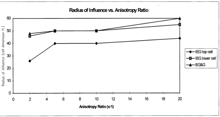
5.5.4 Radius of lnfluence at Various Anisotropy Ratios ... . ..64

5 5 5 Percent Recirculation .. . ... 65

5.5.6 Percent Recirculation at Various Anisotropy Ratios .. ... 65

5.6 D ISCU SSIO N ... ... 68 6. CO N CLU SIO N ... ... 69 REFEREN CES ... ... 70 APPENDIX A: APPENDIX Al: APPENDIX A2: APPENDIX A3: APPENDIX A4: APPENDIX A5: APPENDIX A6: APPENDIX A7: APPENDIX B: APPENDIX B 1: APPENDIX B2: APPENDIX B3: APPENDIX B4: APPENDIX B5: APPENDIX B6: APPENDIX B7: APPENDIX C: COMMAND FILES FOR IEG MODEL SIMULATIONS...73

SAMPLE DYNFLOW COMMAND FILE ... ... 73

CAPTURE WIDTH AT VARIOUS ANISOTROPIES- VELOCITY VECTOR PROFILES ... 75

SAMPLE DYNTRACK COMMAND FILE- CAPTURE AREA ... 78

CAPTURE AREA AT VARIOUS ANISOTROPIES- PARTICLE PLACEMENTS ... 88

SAMPLE DYNTRACK COMMAND FILE- RADIUS OF INFLUENCE/RECIRCULATION ...91

RADIUS OF INFLUENCE AT VARIOUS ANISOTROPIES- PARTICLE TRACKS ... 98

PERCENT RECIRCULATION AT VARIOUS ANISOTROPIES- PARTICLE TRACKS ... 101

COMMAND FILES FOR EG&G MODEL SIMULATIONS ... 104

SAMPLE DYNFLOW COMMAND FILE ... ... 104

CAPTURE WIDTH AT VARIOUS ANISOTROPIES- VELOCITY VECTOR PROFILES...106

SAMPLE DYNTRACK COMMAND FILE- CAPTURE AREA ... 109

CAPTURE AREA AT VARIOUS ANISOTROPIES- PARTICLE PLACEMENTS ...119

SAMPLE DYNTRACK COMMAND FILE- RADIUS OF INFLUENCE/RECIRCULATION.. 122

RADIUS OF INFLUENCE AT VARIOUS ANISOTROPIES- PARTICLE TRACKS... 127

PERCENT RECIRCULATION AT VARIOUS ANISOTROPIES- PARTICLE TRACKS ... 130

LIST OF FIGURES

Figure 2-1: Site Location M ap ... 11

Figure 2-2: M M R Site M ap ... 12

Figure 2-3: Upper Cape Cod Geologic Map... 15

Figure 2-4: Upper Cape Cod Water Table Contour Map... .. ... 17

Figure 2-5: MMR Groundwater Plumes Map... ... 19

Figure 2-6: Extent of C S-10 Plum e ... ... 23

Figure 3-1: Recirculating Well Technology Conceptual Flow Diagram ... ... 25

Figure 3-2: IEG Recirculating Well Technology Conceptual Flow Diagram ... 31

Figure 3-3: EG&G Recirculating Well Technology Conceptual Flow Diagram...34

Figure 5-1: Half-Space Grid Configuration ... 40

Figure 5-2: Vertical Extent of CS-10 Model ... 42

Figure 5-3: IEG V ertical D iscretization ... 44

Figure 5-4: EG&G Vertical Discretization ... 45

Figure 5-5: IEG C apture W idth ... ... 50

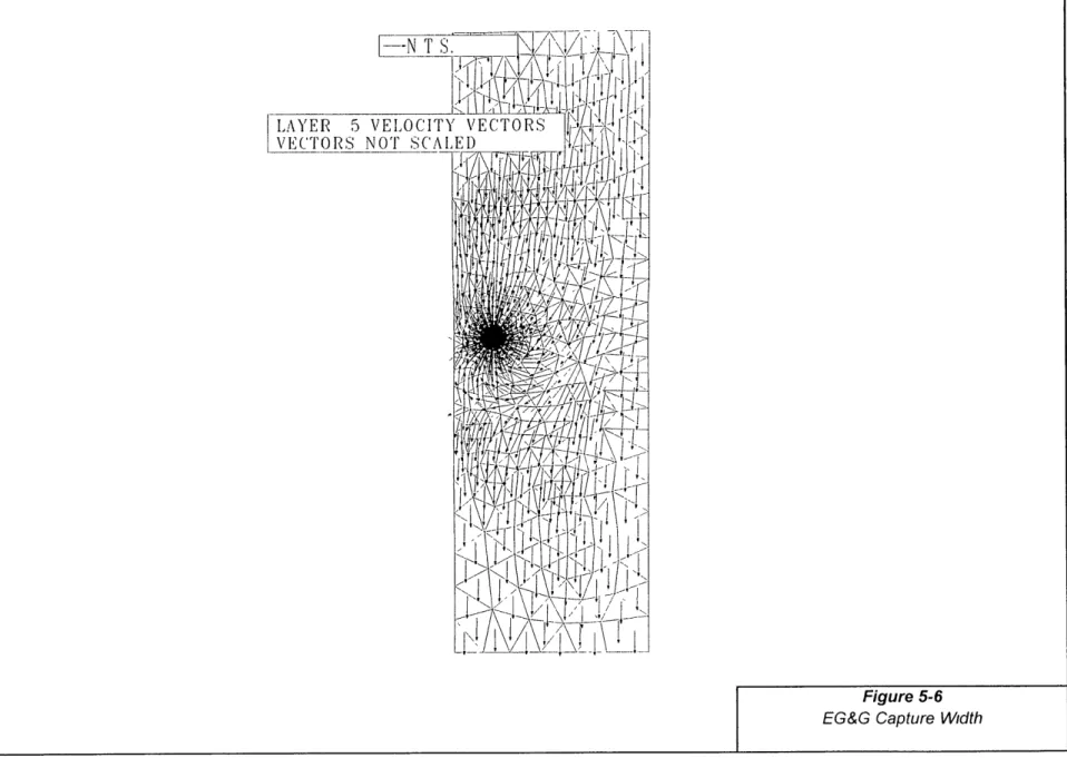
Figure 5-6: EG & G C apture W idth... ... 51

Figure 5-7: Capture Width vs. Anisotropy Ratio... ... ... 52

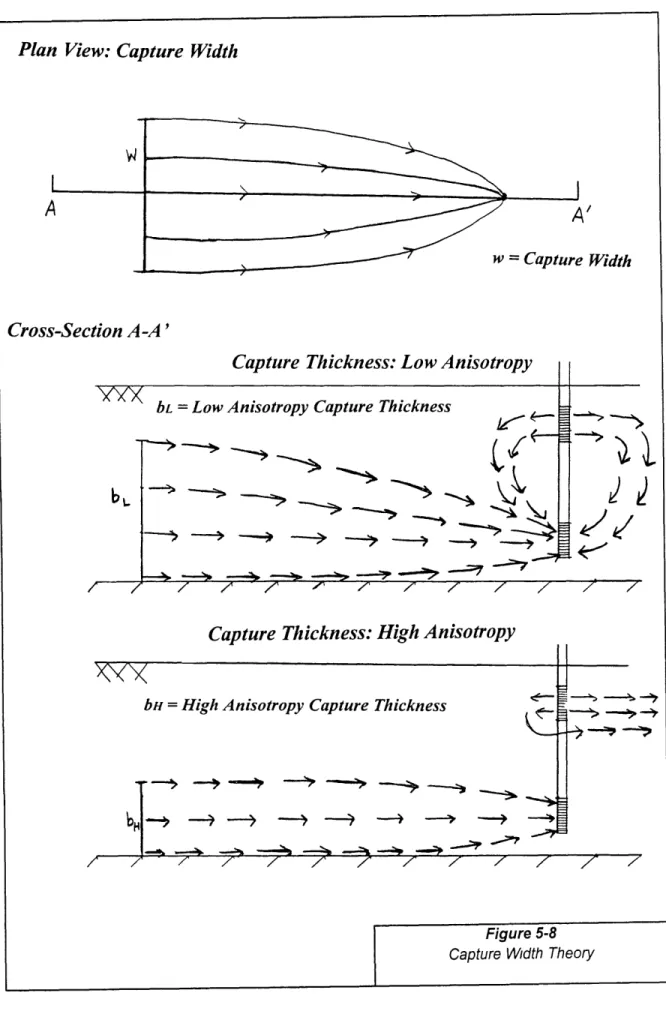
Figure 5-8: Capture W idth Theory ... ... 53

Figure 5-9: IEG Starting and Captured Points ... 55

Figure 5-10: EG&G Starting and Captured Points ... 56

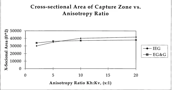
Figure 5-11: Cross-Sectional Area of Capture Zone vs. Anisotropy Ratio ... 58

Figure 5-12: Capture A rea Theory... ... 59

Figure 5-13: Plan View -Radial Placement of Particles ... ... 61

Figure 5-14: IEG Particle Tracks -Horizontal Cross-Section ... .... 62

Figure 5-15: EG&G Particle Tracks -Horizontal Cross-Section ... 63

Figure 5-16: Radius of Influence vs. Anisotropy Ratio ... 64

Figure 5-17: Percent Recirculation vs. Anisotropy Ratio ... 65

Figure 5-18: IEG Particle Tracks -Vertical Cross-Section ... 66

LIST OF TABLES

Table 3-1: IEG Installation Sum m ary... ... 28

Table 3-2: EG&G Installation Summary ... 28

Table 3-3: IEG Circulation Cell Dimensions...32

Table 3-4: EG&G Circulation Cell Dimensions ... 35

Table 5-1: Thickness Distributions ... ... 43

INTRODUCTION

1.1

Problem Definition

The Massachusetts Military Reservation (MMR), located in Cape Cod, Massachusetts, was placed on the National Priorities List (NPL) in 1989 under the Comprehensive Environmental Response, Compensation, and Liability Act (CERCLA). CERCLA, created in 1980, provides guidelines for the remediation of hazardous constituents released from federal facilities. The Installation Restoration Program (IRP) at the MMR includes a number of remediation investigations and has initiated treatment of several of the groundwater plumes on site.

Although in January 1996 Operational Technologies (OpTech) prepared a 60 percent design of a pump and treat containment system for the MMR, residents of Cape Cod feared that the resulting drawdown of the groundwater table would cause ecological damage to the nearby Ashumet Pond (OpTech 1996b). As a result, an investigation began to re-evaluate the pump and treat option and to investigate other containment strategies.

The Technical Review and Evaluation Team (TRET) concurred with the residents and deemed pump and treat technology unacceptable for the MMR due to the potential ecological damage. As an alternative, TRET recommended the evaluation of recirculating well technology. Consequently, a pilot test was initiated at Chemical Spill Area-10 (CS-10) with the purpose of evaluating the potential use of this technology. TRET has acknowledged the advantages of recirculating wells as being capable of in-situ remediation by stripping volatile organic compounds (VOCs) from the groundwater without the need and expense of pumping the groundwater to the surface for treatment. Also, the environmental impact associated with drawdown is eliminated since recirculating wells operate without the need to withdrawal large amounts of groundwater.

1.2

Objectives and Methodology

Recirculating well technology is a new method of in-situ remediation of VOCs in groundwater. Although this technology shows much promise, as cited by TRET, it is still not clearly understood nor is it very predictable. Therefore, it is meaningful to evaluate the many factors that could affect the overall performance and feasibility of recirculating wells. This study focused on the effect that geological characteristics of a particular site have on this technology. Given that the effectiveness of recirculating wells rests on the ability to create large circulation cells within the saturated zone of an aquifer, the anisotropy of a particular site can clearly enhance or limit this capability. Therefore, in order to better understand the relationship between anisotropy ratios and recirculating well performance, various computer simulations were conducted using the DYNSYSTEM groundwater flow software. More specifically, two finite element models were developed to portray the recirculating well designs of IEG Technologies and EG&G Environmental. Once accomplished, particle tracking simulations were executed at various anisotropy ratios to analyze performance criteria such as capture width, capture zone area, radius of influence, and percent recirculation.

In general, velocity vector profiles were generated by simulated heads in DYNFLOW and were used to determine capture widths. In order to conduct particle tracking simulations, efforts were shifted toward DYNTRACK applications. First, a "gate" of contaminant particles were seeded upstream of the recirculating well in order to track which of the particles were ultimately captured by the system. After determining the placement of these particles, the associated areas surrounding these particles were totaled to determine the cross-sectional capture zone area. Secondly, particles were seeded radially about the injection screened intervals of the wells to track the recirculating path of the captured particles. These particle tracks were not only used to estimate the radius of influence that a well could achieve, but they were also utilized to determine the percent of particles that were actually recirculated. From these simulations, performance trends were established to display the effects that anisotropy has on recirculating well technology.

2. BACKGROUND AND SITE DESCRIPTION

This chapter includes background information and site descriptions of the MMR and CS-10

specifically. Before investigating recirculating well technology for use at the MMR, it is essential to have an understanding of the location, history, and physical and environmental conditions of the area of concern.

2.1 MMR Background and Site Description

This section describes the physical and environmental conditions of the MMR. The focus of this section includes location, history of operation, surrounding land use, climate, geography, geology, and hydrogeology of the MMR site.

2.1.1 Location

The MMR lies in the upper western portion of Cape Cod, Massachusetts. It occupies approximately 22,000 acres (35 square miles) within the towns of Bourne, Sandwich, Mashpee, and Falmouth in Barnstable County (see Figure 2-1).

The MMR is divided into four principal areas (see Figure 2-2):

1. Maneuver Range and Impact Area - 14,000-acre site occupying the northern 70 percent of

the MMR. This area is used for training and maneuvers.

2. Cantonment Area - 5,000-acre area located in the southern portion of the MMR. This area

includes administration, operation, maintenance, housing, and support facilities for the base. 3. Airfield - 4,000-acre area located along the southeastern edge of the MMR. This area

contains runways and support facilities for aircraft.

4. Massachusetts National Cemetery - 750-acre area located along the western edge of the MMR. This area contains the Veterans Administration (VA) cemetery and support facilities.

Inset

Cape Cod

Bay

Nantucket Sound

I

-~-~-/

.

CAM=CO

S-BAY

r%-0"W

MASSACHUSETTS

AREARESERATO

BOURNE

_LLS

cos

/r

JuRFM

COW

1

i

4i

®

W

2.1.2 History of Operation

Although military activity at the MMR began in 1911, most of the military operations occurred after 1935 by the U.S. Army, U.S. Navy (USN), U.S. Coast Guard (USCG), U.S. Air Force (USAF), Massachusetts Army National Guard (ARNG), U.S. Air National Guard (ANG), and the Veterans Administration (VA). The level of activity at the MMR has varied over its history. The most intensive U.S. Army activity occurred during World War II (WWII) and the demobilization period after WWII. During this period, the Cantonment Area housed thousands of troops and operated a large motor pool. The USN carried on advances in naval aviation flight training during the last two years of WWII. Also, the USAF maintained an intensive airborne surveillance operation from 1955 to 1970 (CDM Federal, 1993).

Currently, the ARNG and U.S. Army Reserve are conducting a variety of training activities at the MMR. The USCG air station at the MMR provides medium-range search and recovery support of the 1st Coast Guard District and Atlantic Area. The ANG air station at MMR operates and

maintains a squadron of F-15 fighter aircraft to protect the northeastern United States from armed attack. The USAF operates the Precision Acquisition Vehicle Entry - Phase Array Warning System (PAVE-PAWS) for missile and space vehicle tracking. The Veterans Administration also maintains the Massachusetts National Cemetery at the MMR (CDM Federal, 1993).

2.1.3 Surrounding Land Use

Land uses in the area surrounding the MMR include a variety of recreational activities ranging from golfing to hunting. Two adjacent ponds, John's Pond and Ashumet Pond, support swimming, fishing, boating and water skiing. The Shawme Crowell State Forest and Crane Wildlife Management Area support camping, fishing, hiking and mountain biking. Camp Good News, a summer camp for children, is located on Snake Pond.

Besides recreational usage, the land surrounding MMR is also used for agricultural purposes. Most of the agricultural land is used for the cultivation of cranberries. The remaining land is used for the residential, commercial and industrial sector (CDM Federal, 1993).

2.1.4 Climate

The climate at MMR is classified as humid continental. The Atlantic Ocean moderates the temperature; therefore, Cape Cod undergoes warmer winters and cooler summers than inland areas in Massachusetts (CDM Federal, 1993). Also, precipitation is fairly evenly distributed throughout the year, with an average annual rainfall of 46 inches (NCDC, 1990).

2.1.5 Geology and Geography

Western Cape Cod is composed of glacial sediments deposited during the retreat of the Wisconsinan glacier 7,000 and 85,000 years ago. The geology is dominated by three sedimentary units: Buzzards Bay moraine, Sandwich moraine, and Mashpee pitted plain. The Buzzards Bay and Sandwich moraines are located along the north and western edge of Cape Cod, with the Mashpee pitted plain located to the south-east (see Figure 2-3). The Buzzards Bay and Sandwich moraines are composed of ablation glacial till, which is unsorted material ranging from clay to boulder-size rocks, deposited at the leading edge of two lobes of the Wisconsinan glacier. The Mashpee pitted plain is a glacial outwash plain composed of poorly sorted fine to coarse-grained sands. This plain is underlain by fine-coarse-grained glaciolacustrine sediments and base till (CDM Federal, 1993).

The MMR is located on two types of geographic terrain. The Cantonment Area lies on a southward sloping outwash plain with elevations ranging from 100 to 140 feet above sea level. The area north and west of the Cantonment Area lies in the southern portion of the Wisconsinan Age terminal moraines. The presence of irregular hills within this area causes the elevation to range from 100 to 250 feet above sea level, while kettle hole ponds and depressions are found over the entire site (CDM Federal, 1993).

~CAPE

C •~

COD

>.

. •:::::~:::::·::::·:

)II

N

'~~

VIEAD

ON

2.1.6 Hydrogeology

The aquifer system in western Cape Cod is unconfined and recharged by infiltration from precipitation. The high point of the water table occurs as a groundwater mound beneath the northern portion of MMR with groundwater flowing radially outward from the mound peak (see Figure 2-4). The aquifer is bounded by the ocean on three sides, with groundwater discharging into Cape Cod Bay on the north, Buzzards Bay on the west, and Nantucket Sound on the south. Groundwater also discharges into the Bass River in Yarmouth, which forms the eastern lateral aquifer boundary (CDM Federal, 1995).

Surface water at the MMR includes streams and kettle hole ponds in the Mashpee pitted plain. A kettle hole pond is created when buried glacial ice melts and thus creates a local depression. Kettle ponds intersect the water table but cause only local impact on the slope and direction of groundwater flow (CDM Federal, 1995).

The major geology of western Cape Cod is Mashpee pitted plain, which consists of coarse-grained sand and gravel outwash sediment underlain by finer-coarse-grained sediments. The hydraulic conductivity of the outwash sediment measures up to 380 ft/day with a hydraulic gradient range of 0.0014 to 0.0018 ft/ft (E.C. Jordan, 1989) and a net annual recharge of 21 inches (LeBlanc, 1982). The hydraulic conductivity of the underlying fine grained sediment is only 10 percent of the outwash; therefore, the bulk of the regional groundwater is transmitted through the upper outwash layer where the horizontal flow velocities range from 1 to 3.4 ft/day (CDM Federal, 1995).

SCAPE COD BAY " I /4 . A. .. % I *i.*I*.*. \ / I '*.* \ % I, *·. ' \ 111 1 ./... .. 42 4RDS BAY .. _/... •...._{.. •} . "" " . I \- / I \ ,,.N

KEY OBSERVED AVERAGE WATER TABLE CONTOUR IN FEET. DATUM IS SEA LEVEL CONTOUR

INTERVAL 10 FEET. BUZZ N NANTUCXET SOUND SCALE I"= IMILE 0 05 1 Figure 2-4

Upper Cape Cod Water Table Contour Map

I

!

2.2

CS-10 Background and Site Description

This chapter describes the physical and environmental conditions of Chemical Spill-10. Location and site history are also detailed in this section.

2.2.1 Location and Land Use

The CS-10 area of contamination is located adjacent to the northeastern boundary of MMR (see Figure 2-5), within the town of Sandwich, Massachusetts. This plume occupies approximately 38 acres and is currently used for maintenance and storage of vehicles for the ARNG. Approximately 25 ARNG personnel currently work at CS-10 as part of the Unit Training Equipment Site (UTES) operations (CDM Federal, 1993).

The nearest MMR housing is located approximately 19,000 ft southwest of CS-10. The nearest housing area outside of the MMR boundary is located in the Town of Sandwich, with the closest home approximately 650 ft from the eastern fence line. Approximately 75 households are located within a half mile of the CS-10 site in Sandwich. The residences to the east of CS-10 are all served by private wells (CDM Federal, 1993). Residents with drinking water wells in the immediate path of the plume have been placed on public water supply, while other owners of private wells have the option to have their wells tested by the IRP for contamination.

2.2.2 History of Operation

Before 1956, the CS-10 location was occupied by a rifle range. In 1958, the Army Corps of Engineers began constructing the Boeing Michigan Aerospace Research Center (BOMARC) missile facility for the USAF. The BOMARC facility was operated by the USAF from 1960 until it was decommissioned in 1973. In 1973, the facility was transferred from the USAF to the ARNG. In 1978, UTES began their activities at the site (CDM Federal, 1993). The following passages briefly describe the activities that occurred under the two operational periods.

Primary Road

olvent Groundwater Plume

77-- Greater Than MCL Pond

- River/Stream - -- - MMR Boundar 0 5000 10,000 SCALE IN FEET 2.000 4,000 y SCALE IN METERS S n 1 I L . I r r - · - · · -· {%

BOMARC Activities:

In December 1960, the 2 6th USAF Air Defense Missile Squadron began operating the BOMARC

site at the MMR under Strategic Air Command control. Between 1960 and 1973, the USAF maintained 56 BOMARC ground-to-air missile and launcher systems on site (CDM Federal,

1993).

Two models of BOMARC missiles were maintained at the MMR. The BOMARC-A missile, a nuclear-warhead-capable missile, was powered by both a liquid-fuel rocket booster and a ramjet engine. This missile was stationed at MMR beginning in 1960 and then phased out and replaced by BOMARC-B. The BOMARC-B was also a nuclear-warhead-capable missile but used a solid-fuel rocket booster. The BOMARC-B model was operational from 1962 to 1972. Because of the classified nature of the site activities, little public information exists regarding system operations and maintenance activities, but existing building design plans provide good indication of past actions. The operations that seemed to generate the most hazardous waste at the BOMARC facility were missile guidance system maintenance, engine maintenance, and fueling and defueling operations (CDM Federal, 1993).

The maintenance of the guidance system would have required the use of halogenated solvents. Common solvents used by the military during this time period would most likely have been methylene chloride, 1,1,1-trichloroethane (TCA), trichloroethene (TCE), and tetrachloroethene (PCE). It is possible that the military switched to a freon-type solvent like chlorofluoromethane in the last few years of the BOMARC facility activities (CDM Federal, 1993).

The BOMARC-A missile ramjet engine used JP-4 jet fuel. JP-4 contains benzene, toluene, ethylbenzene, xylene, naphthalene, 2-methylnaphthalene and other hydrocarbons. JP-4 waste was generated as a result of refueling and maintenance and was disposed of by means of a leaching field. The BOMARC-A missile also used liquid fuel to boost the missile to its cruising speed before the ramjet engine would take over and propel the missile to its target. This liquid fuel, Aerozine 50, reacted with a strong oxidizing agent, red-fuming nitric acid (RFNA), to produce the force needed to propel the rocket. Aerozine 50 consists of a 50:50 mixture of

hydrazine and unsymmetrical dimethylhydrazine (UDMH). Waste RFNA was disposed in a neutralization pit containing crushed limestone. Waste hydrazine and UDMH were pumped into a waste fuel tank and released at a slow rate into a spill pit to allow complete auto-oxidation to occur (CDM Federal, 1993).

Other potential sources of site contamination at CS-10 from BOMARC activities include vehicle fueling, vehicle maintenance and power plant operation. While these activities are likely sources of contamination, no documents exist to indicate the amount of waste produced or if any fuel spills occurred (CDM Federal, 1993).

UTES Activities:

The UTES maintenance shop began operating at the BOMARC site in 1978. UTES is responsible for the maintenance of 300 to 350 armored and wheeled vehicles used for the ARNG training activities at MMR. Waste generated by UTES activities include waste oil, halogenated solvents, petroleum distillate solvents, battery electrodes, paints, and paint removal solvents. Over the years the stored waste has been transferred and transported many times and has consequently caused the contamination of approximately 25 cubic feet of soil. After the decommissioning of the main 500 gallon storage trailer in 1985, the contaminated soil was removed. Currently, UTES collects its waste in 55 gallon drums and stores them at the Camp Edwards Temporary Hazardous Waste Storage Facility before they are shipped to an off-site disposal area (CDM Federal, 1993).

2.2.3 Nature and Extent of the CS-10 Plume

The current understanding of the overall nature of the CS-10 groundwater plume is documented in the Remedial Investigation (RI) report for the UTES/BOMARC and BOMARC Area Fuel Spill AOC CS-10 Groundwater Operable Unit (CDM Federal, 1995). TCE, PCE, and 1,2-DCE were the primary chlorinated organic contaminants detected in the field work that was conducted in 1993. Other organic contaminants detected included 1,1-DCE, trans-1,2,-DCE, and trimethylbenzene. When the RI was conducted, total contaminant concentrations were detected,

with TCE being the main contaminant having a maximum concentration of 3,200 ug/L. The maximum concentration of the next single contaminant was PCE at 500 ug/L.

The TCE "hot spot" was tracked downgradient of the well that measured 3,200 ug/L, but screened auger sampling did not detect TCE or any other chlorinated VOCs at those wells. Deep TCE contamination, however, was encountered during drilling at depths in excess of 105 feet below the water table (-55 feet mean sea level (MSL)). The extent of the deeper portions of the plume are still being defined through data gap field efforts.

The CS-10 plume is migrating primarily through the unconfined Mashpee Pitted Plain glacial outwash sand and gravel aquifer. The top of the plume is approximately at sea level and the base of the plume is at or within the underlying fine-grained glaciolacustrine sediments that form the base of the Mashpee Pitted Plain. Based upon TCE concentrations greater than 5 ug/L, the plume is currently estimated to be approximately 16,500 feet long, with a maximum width of 4,200 feet, and a thickness of about 120 feet (see Figure 2-6). The CS-10 plume includes an eastern lobe, whose leading edge has migrated underneath Ashumet Pond, and a western lobe that appears to be migrating in a south-southwesterly direction.

Solvent Groundwater Plume I- Greater Than MCL ~ Prtmary Road

O

3.

RECIRCULATING WELL TECHNOLOGY

Recirculating well technology is a new method for in-situ remediation of volatile organic compounds (VOCs). The treatment system primarily removes VOCs from groundwater by the physical process of air stripping. The basic recirculating well relies on pressurized air to lift water through the well and promote the transfer of VOCs from the liquid phase to the vapor phase (see Figure 3-1). Groundwater enters the well through the extraction screened opening and is lifted upward by the pressurized air. The diffused air bubbles strip the VOCs from the groundwater. The vapor phase is then collected and treated aboveground while the groundwater is returned to the aquifer through the injection screened opening. In addition to air stripping, the aeration of groundwater stimulates aerobic biodegradation (Jacobs Engineering, 1996).

The following sections discuss the advantages of this technology, the history, and the specific designs of the two recirculating wells being considered for the MMR: IEG Technologies and EG&G Environmental.

Air Inlection CO, Addition for Scaling Control (If require Recharge A from Blowe Vadose Zone Clean Saturated Zone VOC Contaminated Water -

I' 1

Lower Recirculating Well Technology

Extraction Screen I Conceptual Flow Diagram

L-IUl 93" I '1 risen ~lr

3.1

Advantages of Recirculating Wells

Recirculating wells have many advantages over the traditional pump and treat systems and air sparging systems. The advantage derives from the means in which VOCs are treated. As stated in the previous section, the recirculating well technology is an in-situ method of treating VOCs whereby contaminated groundwater is extracted from one screened interval, treated within the well, and re-injected at another screened interval in the same well. However, unlike recirculating well technology, pump and treat systems extract contaminated groundwater, bring the groundwater to the surface, treat it, then re-inject the treated groundwater at another location at the site. In addition, air sparging is dissimilar in that it treats contaminants without physically capturing any groundwater. The following sections detail more specifically the advantages of recirculating wells.

3.1.1 Advantage over Pump and Treat Systems

Recirculating wells have numerous physical and cost advantages over pump and treat systems. First of all, since recirculating wells strip VOCs without extracting large amounts of groundwater, the environmental impact associated with drawdown is eliminated. This is quite favorable since water table drawdown can impact wetlands, water resources, saltwater intrusion and foundation settlement. Secondly, creating local groundwater recirculation is another key advantage of recirculating wells. The induced vertical flow effectively flushes out larger areas since it can overcome horizontal heterogeneities. As a result, time and cost of remediation may be reduced. In addition, biodegradation is enhanced because the groundwater that is recirculated in the aquifer is saturated with dissolved oxygen. Consequently, biodegradation can reduce the time and cost associated with remediation. Also, recirculating well technology does not require groundwater to be pumped to the surface; therefore, the cost associated with permitting and monitoring of groundwater extraction and reinjection is reduced. Finally, because recirculating wells extract and inject within the same well, the capital cost is greatly reduced compared to a standard pump and treat system that requires separate extraction and injection wells (Metcalf and Eddy, 1996).

3.1.2 Advantage over Air Sparging

Recirculating wells have many physical and cost advantages over air sparging systems as well. Because recirculating wells remove groundwater from the surrounding media, the air is able to contact the groundwater without the interference caused by the soil particles. The greatest limitation of an air sparging system is the phenomenon know as air channeling. When air travels through soil, it chooses the path of least resistance. Once the path is established, air will tend to travel though this channel. By removing groundwater from the soil media, air channeling is reduced; therefore, recirculating wells are more reliable than air sparging systems (Metcalf and Eddy, 1996).

Another advantage of recirculating wells is its ability to induce groundwater to travel horizontally and vertically; therefore, contaminant plumes can be contained. Air sparging systems cannot accomplish this type of containment. Also, the horizontal component of the flow gradient is effective in flushing a greater horizontal extent than air sparging. As a result, time and cost of remediation may be reduced. In addition, recirculating wells are cheaper to install since extraction and injection are performed in one well, compared to a two-well air sparging system. Air sparging requires an air injection well and a soil vapor extraction well, thus resulting in a larger capital cost (Metcalf and Eddy, 1996).

Finally, recirculating wells can be installed in deep aquifers, whereas sir sparging systems cannot. Air sparging systems are limited to the vadose zone or to plumes near the phreatic surface of an aquifer. Recirculating wells, on the other hand, can be installed to remediate the vadose zone as well as deep plumes in both phreatic and confined aquifers (Metcalf and Eddy,

1996).

3.1.3 Lack of Case History

Currently, only two companies in the world, IEG Technologies Corporation and EG&G Environmental, hold patents on recirculating well designs. Recirculating wells have been used in Germany for ten years, whereas in the United States use is still very limited (see Tables 3-1 and 3-2 for list of installations and dates if available). Due to the lack of pilot test studies conducted

in the U.S., MMR is proceeding with this technology with caution and thereby conducting a pilot test of both IEG and EG&G's equipment to allow the best design for CS-10 to emerge.

Table 3-1: IEG Installation Summary

Date Location Type of Geology Contaminant Horizontal Total

System - Hydraulic Depth

Conductivity

(cm/See) > (Feet) 1992 Gas Station UVB 400 Saprolite Gasoline 1 0 x 10-4 41

Troutman, NC Single Pump Clayey Silt with Sand

1993 USAF UVB 400 Alluvial Fan Chlorinated 7 5 x 10-3 81 7 Riverside, CA Single Pump Silty Sand Hydrocarbons

1993 Confidential UVB 400 Saprolite Chlorinated 1 8 x 10-3 133 5

Charlotte, NC 3-Screens Silty Sand with Hydrocarbons Single Pump Clay

1994 W R Grace UVB 400 Saprolite Gasoline 1 0 x 10-4 49 Chester, SC Single Pump Silty Clay with

Clay

1995 U S Navy UVB 400 Fine to Medium Creosote 1 0 x 10-3 25 Gainesville, FL Single Pump Sand

1995 New York State UVB 400 Fine to Med Sand BTEX 8 8 x 10-3 30 Yonkers, NY Single Pump to Sandy Gravel

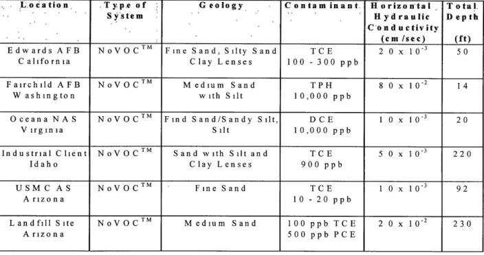
Table 3-2: EG&G Installation Summary

L)Location ,Type of G eology Contam inant Horizon'tal Total. S

System Hydraulic Depth

C'on d uctivity

_ __ (cm fsee) (ft)

TM 3

Edwards AFB NoVOC Fine Sand, Silty Sand TCE 2 0 x 10- 50

California Clay Lenses 100 - 300 ppb

Fairchild AFB NoVOC T M

Medium Sand TPH 8 0 x 10-2 14

W ashington with Silt 10,000 ppb

Oceana NAS NoVOC T M

Find Sand/Sandy Silt, DCE 1 0 x 10-3 20

Virginia Silt 10,000 ppb

Industrial Client NoVOC Sand with Silt and TCE 5 0 x 10-3 220

Idaho Clay Lenses 900 ppb

USMC AS NoVOCTM Fine Sand TCE 1 0 x 10- 3 92

Arizona 10 - 20 ppb

Landfill Site NoVOCTM Medium Sand 100 ppb TCE 2 0 x 10-2 230

3.1.4 Performance Limitations

Physical and chemical properties of contaminants, as well as site characteristics, may enhance or limit the performance of recirculating well technology.

Contaminant Properties:

Air stripping is the dominant process by which the recirculating well system removes organic contaminants from the groundwater. Therefore, it is important for the contaminants of concern to be sufficiently volatile so that they may partition into the air stream and be removed by the vacuum extraction to achieve successful remediation. Since BTEX compounds are relatively volatile, this technology works well for gasoline and other hydrocarbon contaminants. The recirculating well system also removes non-volatile contaminants that undergo biologically mediated transformations under aerobic conditions. Overall, the volatility and the biodegradation of the individual compounds must be considered as part of the recirculating well design to ensure that appropriate remediation is achieved (Jacobs Engineering, 1996).

Hydrogeologic Setting:

Successful operation of the recirculating well depends on the hydrogeologic conditions of the site. Site-specific properties, such as contaminated aquifer thickness, stratigraphic uniformity, hydraulic conductivities, and groundwater velocity, will influence the performance of the recirculating well.

The thickness of the contaminated plume will affect the size and placement of many of the design features. The recirculating well is designed to draw water from the base of the plume and discharge it at the surface of the plume. Circulation is most effective when the soil beneath the recirculating cell is relatively impermeable. Also, flow rates through the well must be sufficient to ensure that a portion of the discharged water from the upper screen recirculates back through the lower screen. In addition, the recirculating well system is designed to operate through relatively homogeneous aquifer layers. Therefore, the presence of stratigraphic heterogeneities between the upper and lower screened intervals may restrict the recirculation pattern.

3.2 Design and Use at MMR

The following sections describe IEG Technologies' recirculating well design features, then detail the aspects of EG&G Environmental's design.

3.2.1 IEG Technologies Corporation

SPB Technology, Inc., a licensed representative of IEG Technologies Corporation, has installed two UVB (German acronym for vacuum-vaporized well) systems for the CS-10 groundwater contaminated plume at the MMR site. The UVB system used at the MMR incorporates a specially adapted groundwater well that utilizes three screened casing sections, a groundwater stripping reactor, an aboveground blower, and a contaminant vapor collection system (see Figure 3-2). The centrifugal blower at the ground level provides negative pressure for the system and is used to remove the contaminated air from the well vault. The negative pressure causes atmospheric air to enter the well through the air pipe. The fresh air pipe is connected to a stripping reactor which forms air bubbles as it jets through the pin hole plate and mixes with influent groundwater. There is a mass transfer of contaminants from the water phase to the air phase as bubbles expand and release the VOCs in "the upper portion of the well. The contaminated vapor is then transported by air flow to an aboveground carbon absorption treatment system (Jacobs Engineering, 1996).

Because of the three-screen casing design, two types of circulation cells are developed: a standard (clockwise) circulation cell on top of a reverse (counter-clockwise) circulation cell. The middle screen is installed in the vertical center of the plume. A pump is positioned in the center of the six-foot screen and packed off from the remaining well casing to create a reduced hydraulic head zone. The water is pumped to the UVB air stripping system, located near the ground surface within the well vault, where VOCs are removed from the groundwater. After air stripping, the water is split into two streams and each stream falls back down to either the upper or lower well screen. Because there are two areas of increased head and one area of reduced head, water flows horizontally and vertically into the center of the well and creates two circulation cells (Jacobs Engineering, 1996).

UVB

Figure 3-2

lEG Recirculating Well Technology Conceptual Flow Diagram

LAND SURFACE

UVB

LABYRINTH-PUMPS

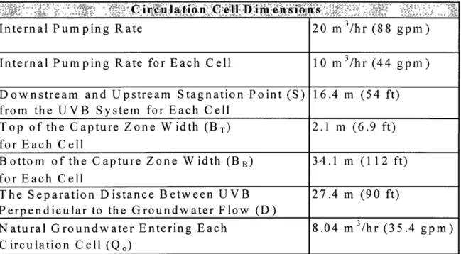
IEG Technologies estimated the circulation cell dimensions using the well design and the aquifer parameters. The capture zone bottom width BB, and top width BT, are estimated at an upstream distance from the UVB system of five times the height of the plume. The distance, S, is the stagnation point upstream and downstream of the UVB system and is used as the maximum expansion of the sphere of influence of the UVB system. Models developed by Herrling are used to estimate the size of the capture, treatment, and release zones, the stagnation point, and time of particle travel (Herrling, 1991). The calculations for the CS-10 pilot study were performed using a proprietary software program. The estimated cell dimensions for the two IEG wells installed at MMR are shown in Table 3-3 (Jacobs Engineering, 1996).

Table 3-3: IEG Circulation Cell Dimensions

Internal Pumping Rate 20 m 3/hr (88 gpm)

Internal Pumping Rate for Each Cell 10 m3/hr (44 gpm) Downstream and Upstream Stagnation Point (S) 16.4 m (54 ft) from the UVB System for Each Cell

Top of the Capture Zone Width (BT) 2.1 m (6.9 ft) for Each Cell

Bottom of the Capture Zone Width (BB) 34.1 m (112 ft) for Each Cell

The Separation Distance Between UVB 27.4 m (90 ft) Perpendicular to the Groundwater Flow (D)

Natural Groundwater Entering Each 8.04 m 3/hr (35.4 gpm) Circulation Cell (Qo)

3.2.2 EG&G Environmental

Metcalf and Eddy, a licensed representative of EG&G Environmental, has installed two EG&G NoVOCsTM systems for the CS-10 groundwater contaminated plume at the MMR site. The NoVOCsTM system used at the MMR incorporates a dual casing design with two screened intervals, a diffuser, an aboveground blower, and a contaminant vapor collection and treatment system (see Figure 3-3). The aboveground blower is used to remove the contaminated air from the recirculating well so the air can be treated by a carbon absorption system. Once the air is treated, it is then injected back into the NoVOCsTM system. It is this treated air that is used to strip the VOCs from the groundwater. The treated air pipe is connected to a diffuser which forms air bubbles and mixes with influent groundwater. There is a mass transfer of contaminants from the water phase to the air phase as bubbles expand and release the VOCs in the upper portion of the NoVOCsTM well (Jacobs Engineering, 1996).

Because of the two-screened-interval design, a clockwise circulation cell develops. The bottom screen is installed near the bottom of the plume. A pump is positioned in the center of the bottom screen to create a reduced hydraulic head zone. The water is then pumped through the inner 6-inch casing, to the top of the NoVOCsTM well, where VOCs are removed from the groundwater. After air stripping, the treated groundwater falls out of the inner 6-inch casing into the outer 10-inch casing where it travels down to the upper screen. This significant hydraulic pressure forces the water horizontally into the aquifer through the upper screen, and owing to areas of increased and reduced head, water flows horizontally and vertically into the bottom screen and creates the circulation cell (Jacobs Engineering, 1996).

CLEAN AIR FROM 8LO•R

VOC-CONTAMINATED AIR

TREATED WATER

STRIPPING ZONE. AIR-WATER MIXTURE

~~ UNCONTAMINATE~D_{AIR OR WATER}

A OR WATER

-- ~-- AIR-WATER MIXTURE

Figure 3-3

EG&G Recirculating Well Technology Conceptual Flow Diagram

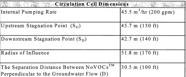
EG&G Environmental calculated the circulation cell dimensions based on the aquifer parameters. The radius of influence is the maximum horizontal distance the recirculating well affects the groundwater flow. The distance Su is the stagnation point upstream, and the distance SD is the stagnation point downstream of the NoVOCsTM system. The determination of the size of the radius of influence is based on dimensionless curves developed by MODFLOW, a numerical groundwater flow model. Table 3-4 shows the estimated circulation cell dimensions for each of the EG&G Environmental NoVOCsTM systems installed at the MMR (Jacobs Engineering,

1996).

Table 3-4: EG&G Circulation Cell Dimensions

Circulation Cell Dimen;sons

Internal Pumping Rate 45.5 m3/hr (200 gpm)

Upstream Stagnation Point (Su) 45.7 m (150 ft)

Downstream Stagnation Point (SD) 42.7 m (140 ft)

Radius of Influence 51.8 m (170 ft)

The Separation Distance Between NoVOCsTM _{30.5 m (100 ft)}

Perpendicular to the Groundwater Flow (D)

4.

NUMERICAL MODELING APPROACH

4.1

Introduction

In order to predict the effectiveness of recirculating well technology at CS-10, groundwater flow modeling was performed. Computer modeling is an effective and cost-efficient means to anticipate the performance as well as determine the conditions in which this technology would most efficiently perform. Hydrogeological conditions can enhance or limit a recirculating well's capability; therefore, by coupling numerical models with particle tracking simulations, favorable hydrogeologic parameters can be determined for recirculating well use at a particular contaminated site.

The interaction of hydrogeologic conditions affecting the hydraulics of the recirculating well technology was investigated in this study. Since two recirculating well designs are being considered for use at CS-10, two corresponding 3-D finite element groundwater flow models were developed: one to represent IEG Technologies, Inc. and the other to simulate EG&G Environmental.

4.2

Description of Modeling System

Groundwater flow in the Chemical Spill-10 vicinity of the MMR was simulated using the three-dimensional, finite element DYNSYSTEM software. Camp, Dresser & McKee developed this dynamic groundwater flow simulation model as a tool for analyzing a variety of groundwater flow applications, such as coal strip mine dewatering projects, regional groundwater supply studies, pump test evaluations, vertical consolidation estimates, analyses of flow in fractured rock, and hazardous waste remediation studies (CDM Inc., 1994). For the case of CS-10, DYNSYSTEM was used to simulate the hydraulics of recirculating well technology to determine the effectiveness of contaminant particle capture and recirculation.

The DYNSYSTEM is composed of three sets of code, DYNFLOW, DYNPLOT, and DYNTRACK, as discussed in the following sections.

4.2.1 DYNFLOW

DYNFLOW is a computer program coded in the FORTRAN language that uses the Galerkin finite element formulation to simulate three-dimensional groundwater flow. Based on conventional flow equations in porous media, DYNFLOW can simulate equilibrium or transient responses of groundwater flow systems to various types of stresses. These stresses include induced infiltration from streams, artificial and natural recharge or discharge, pumping and evapotranspiration. This program uses linear finite elements and solves both linear (confined) and non-linear (unconfined) aquifer flow equations. DYNFLOW uses a trapezoidal time stepping scheme with both lumped and distributed storage term options. The program handles multi-level pumpage using one-dimensional elements, and can treat general anisotropy in terms of hydraulic conductivity (CDM Inc., 1994).

4.2.2 DYNPLOT

DYNPLOT serves as a graphic interface and geographic information system for the DYNSYSTEM groundwater models. It is a graphical pre- and post-processor that supports the groundwater flow and contaminant transport models DYNFLOW and DYNTRACK (CDM Inc., 1994). DYNPLOT creates displays in plan and cross-sectional views of various forms of data, such as measured field data, model input data, and results from previous simulations.

In building the numerical model for CS-10, DYNPLOT was first used to generate a grid by utilizing its automated grid generation and grid editing capabilities. Also, after each DYNFLOW and DYNTRACK simulation was conducted, DYNPLOT was used to graphically present the output of the run.

4.2.3 DYNTRACK

DYNTRACK is a companion mass transport program that simulates the spread of contaminants in the saturated zone using flow fields generated by DYNFLOW. DYNTRACK utilizes the same three-dimensional finite element grid representation of aquifer geometry, flow field, and stratigraphy used for the DYNFLOW model (CDM Inc., 1984). The particle tracking function is

used in this model to follow the path of the conservative constituents. This enables DYNTRACK to determine an expected location of the contamination as well as an estimated time of travel.

5. GEOLOGICAL PARAMETER MODEL

5.1

CONCEPTUAL MODEL

Since the conceptual model dictates the shape that the DYNFLOW data and commands must follow, it is essential that it is clearly defined. The main motivation behind the grid design for the geologic parameter model was to simulate and predict the CS-10 pilot test results. However, the pilot test data were not available, so only initial head values were incorporated into the model, while more sophisticated model calibrations were unable to be conducted. Nevertheless, running the model with the pilot test configuration still provided significant understanding of recirculating well operations. More specifically, it generated general trends concerning capture widths, cross-sectional areas of capture zones, radius of influences, and recirculation efficiencies under various anisotropy ratio schemes.

The following parameters were specified in the conceptual model.

5.1.1 Geometric Boundaries

Horizontal limits of a grid must be set at points sufficiently far from the area of interest or at boundaries where the head or flux conditions are known. This is to ensure that the boundary conditions do not affect or limit the activity range within the region of interest. Currently at the CS-10 pilot test site, two different recirculating well technologies are being tested side by side (IEG and EG&G) with two wells of each design being tested. Since each vendor's proposal differs significantly from the other, the vertical discretization was modified for each design. In order to simplify each model, a "half-space" grid was generated. In other words, only half the area of interest was specifically modeled taking advantage of the symmetry created by a two-well system (see Figure 5-1). The first horizontal limit was chosen at the no flow boundary that lies directly between the two wells. IEG and EG&G each installed their two wells approximately 90 feet apart; therefore, a lateral no-flow boundary of the model was set at 45 feet from the well. Next, since it is anticipated that the circulation cell radius, or radius of influence, of each

____ 1 I - 0I - 20 10 -F0O( -'100 -:100 -0(0 - IOU0 0 Groundwater Flow

4,

operating well, subjected to the natural conditions of the site, will be between 50 and 100 feet, the opposite lateral limit was set at 200 feet from the well to allow sufficient room for the well activity. Finally, the horizontal boundaries upgradient and downgradient from the well were set 400 feet away from the recirculating well to allow for ample transitional space from uniform regional to local radial groundwater flow to occur in the modeled region.

Vertical limits of a grid depend both on the horizontal limits as well as on the site stratigraphy. The upper vertical limit was set at ground surface elevation, while the lower boundary was specified at the impervious bedrock (see Figure 5-2). The thickness of the modeled region is 270 vertical feet, which includes the 120 ft. thick contaminant CS-10 plume as well as the remaining sediments overlying it. Overall, the dimensions of the model are 800 feet long by 245 feet wide by 270 feet high, resulting in a total bulk volume of 53 million cubic feet.

5.1.2 Hydraulic Boundaries

The ground surface in the model is represented by a "rising" boundary condition. Setting a rising head condition at the surface stops the head from rising above this elevation and effectively allows surface discharge at that node (CDM Inc., 1994). Also, as noted in Figure 5-1, the boundaries parallel to the groundwater flow are designated as no flow, while the boundaries perpendicular to the regional flow are assigned fixed heads, which are based on the natural hydraulic gradient of the area.

5.1.3 Grid Generation and Discretization

The finite element grid for the numerical model consists of radially spaced nodes about the recirculating well. The grid spacing ranges from tens of feet at the boundaries of the model to fractions of feet near the well to allow for greater detail about the area of interest. In all models, areas of interest require more discretization to account for the rapidly changing conditions that occur at these areas, both in the horizontal and vertical directions. Figure 5-1 graphically displays the plan view of the grid created.

Modeled Thickness

Plume Thickness

r

The model consists of 18 layers and 19 levels. The defined levels extend from bedrock to the ground surface. Again, more detail is desired in the areas of interest, which are the screened sections of the vertical well. Therefore, a range between 5 and 15 foot intervals was initially defined along the well, where screened sections were discretized into 5 foot intervals and areas between the screens up to 15 foot intervals. Not much activity was anticipated in the saturated area between the top of the well and the water table level, so much thicker layers were defined in that section of the vertical extent. However, once the DYNFLOW command files were executed, the head values were checked along the well node and the level elevations were adjusted in the areas of rapidly changing head. A cross-sectional view of the IEG and EG&G model grids displaying the discretization is shown in Figures 5-3 and 5-4, respectively.

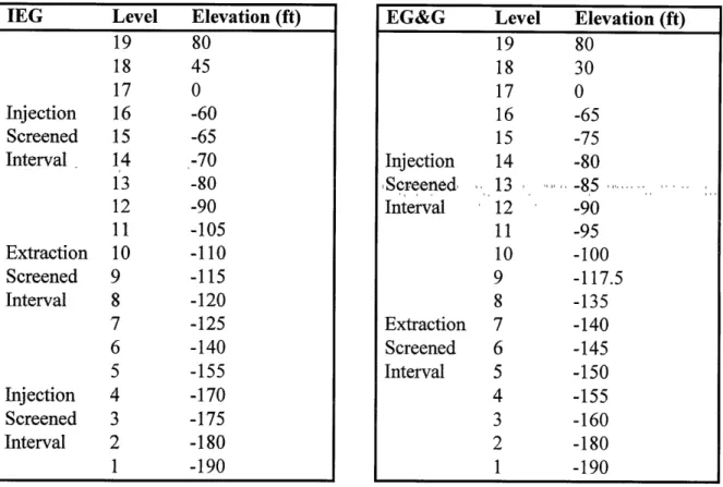
The specific thickness distributions of the two recirculating well designs are detailed in Table 5-1. Note that levels start at bedrock up to the ground surface, and all elevations are relative to mean sea level.

Table 5-1: Thickness Distributions IEG Level Elevation (ft)

19 80 18 45 17 0 Injection 16 -60 Screened 15 -65 Interval 14 -70 13 -80 12 -90 11 -105 Extraction 10 -110 Screened 9 -115 Interval 8 -120 7 -125 6 -140 5 -155 Injection 4 -170 Screened 3 -175 Interval 2 -180 1 -190

EG&G Level Elevation (ft)

19 80 18 30 17 0 16 -65 15 -75 Injection 14 -80 ,Screened 13 -85 ... Interval 12 -90 11 -95 10 -100 9 -117.5 8 -135 Extraction 7 -140 Screened 6 -145 Interval 5 -150 4 -155 3 -160 2 -180 1 -190

GO - 0 - • "-_ Injection

Interval-O-

-1-

a80 40 0 20 0 ---- -- - - - -320 -s 0 -Injection Interval==

-- 20

1

0-

__

-L_

---

--

r__4

~---5.2

Design Parameters

5.2.1 Pumping Rates

Each recirculating well design calls for different pumping rates with different numbers of screened intervals. For instance, IEG's well design develops two circulation cells operating at 44 gallons per minute (gpm) each. On the other hand, EG&G's design creates only one circulation cell and it is pumped at a maximum of 200 gpm. For either case, the nodes corresponding to the extraction and injection sections of the vertical circulation well were assigned negative and positive pumping values, respectively.

In addition, one-dimensional elements, with high conductivity values, were defined at the screened intervals of the wells so that significant head differences would not occur across these areas. As a result, a more accurate simulation of injection and extraction was achieved.

5.2.2 Screened Intervals

IEG's recirculating well design utilizes four, 10-ft. screened intervals, while the EG&G well only has two, 15-ft. screens. The number of circulation cells developed by each design impacts the radius of influence that each recirculating well can achieve (see Figures 3-2 and 3-3).

5.3 Aquifer Parameters

5.3.1 Aquifer Thickness

The unconfined aquifer underlying CS-10 is 270 feet in total thickness. The model extends throughout the thickness of the aquifer and therefore incorporates the entire interval that lies between bedrock and the ground surface (see Figure 5-2).

5.3.2 Hydraulic Conductivity

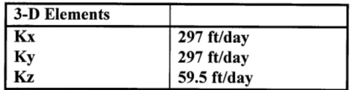
The hydraulic conductivities in the CS-10 area were defined as shown in Table 5-2.

Table 5-2: CS-10 Hydraulic Conductivities 3-D Elements

Kx 297 ft/day

Ky 297 ft/day

Kz 59.5 ft/day

Note that for the screened areas of the wells, 1-D elements were conductivities of 10 million ft/day. This conductivity value was set at eliminate significant head differences across each screen.

defined with very large this high level in order to

The anisotropy ratio between the horizontal and vertical directions is approximately 5:1 in this region, according to the CS-10 Final Report. As proven later, the anisotropy of a site strongly influences the effectiveness of recirculating well operations.

In addition, since the aquifer associated with CS-10 consists of a homogeneous distribution of fine to coarse grained sand, only this one type of material was defined in the model. Therefore, the hydraulic conductivity values above represent the entire extent of the modeled aquifer.

5.3.3 Hydraulic Gradient

Since the natural head drop of the CS-10 area is understood to be approximately 1 ft/day, or more specifically to have a hydraulic gradient of 0.0014 ft/ft, the overall head drop across the 800 ft.